


Abstract
Generalization of transcriptomics results can be achieved by comparison across experiments. This generalization is based on integration of interrelated transcriptomics studies into a compendium. Such a focus on the bigger picture enables both characterizations of the fate of an organism and distinction between generic and specific responses. Numerous methods for analyzing transcriptomics datasets exist. Yet, most of these methods focus on gene-wise dimension reduction to obtain marker genes and gene sets for, for example, pathway analysis. Relying only on isolated biological modules might result in missing important confounders and relevant contexts. We developed a method called Plant PhysioSpace, which enables researchers to compute experimental conditions across species and platforms without a priori reducing the reference information to specific gene sets. Plant PhysioSpace extracts physiologically relevant signatures from a reference dataset (i.e. a collection of public datasets) by integrating and transforming heterogeneous reference gene expression data into a set of physiology-specific patterns. New experimental data can be mapped to these patterns, resulting in similarity scores between the acquired data and the extracted compendium. Because of its robustness against platform bias and noise, Plant PhysioSpace can function as an inter-species or cross-platform similarity measure. We have demonstrated its success in translating stress responses between different species and platforms, including single-cell technologies. We have also implemented two R packages, one software and one data package, and a Shiny web application to facilitate access to our method and precomputed models.
Introduction
As a consequence of their nonmotile nature, plants developed a highly organized yet labyrinthine response system to external biotic and abiotic stresses (Pérez-Clemente et al., 2013). Exploiting this complex system has been playing an important role in achieving sustainable plant protection in agriculture. Instances of tweaking the plant defense system for obtaining better crops are numerous. For instance, priming, that is, promoting plants to a primed state of defense, has been known, investigated, and utilized for decades, if not centuries (KUĆ, 1987; Chester, 1933). By exposure to biotic stresses (e.g. microbe-, pathogen-, and herbivore-associated molecular patterns) or abiotic stresses (for instance, harsh temperatures, drought, or damage-associated molecular patterns), plants switch to a primed, reinforced defense state. In this primed state, they can display sharper stress responses and become more robust and resilient organisms. By artificially exposing plants to biotic and abiotic stresses directly, or to some natural or synthetic chemicals that provoke the same defense response, it is possible to engineer sturdier plants (Conrath et al., 2015). Another example of crop engineering occurs by genetically modifying (GM) plants to attain higher tolerance to stress (Datta, 2013). Introducing a single gene encoding C-5 sterol desaturase (FvC5SD) from Collybia velutipes to tomato (Solanum lycopersicum) is an instance of GM crop research, and it brings about a drought-tolerant and fungal-resistant crop (Kamthan et al., 2012a, 2012b). Obtaining resistance to papaya ringspot virus (PSRV) in transgenic papaya (Carica papaya L.) is another famous example. The resistant papaya gains protection by expressing the PSRV coat protein transgene (Gonsalves, 1998).
In research experiments aiming to modify the plant’s defense system, such as the examples mentioned above, the stress responses of plants under study are thoroughly examined and contrasted to wild-types (WTs). We argue that a tool that is capable of quantitatively and dependably measuring the speed and intensity of stress responses in plants can be of great assistance in this field of research. Hence, we present Plant PhysioSpace, an advanced computational tool based on PhysioSpace (Lenz et al., 2013), for quantitative analysis of stress responses in plants.
Sequencing technologies are commonly used for studying the changes in the plants under examination. However, analysis of the resulting data is mostly focused on gene-wise dimension reduction to obtain a list of genes, with the rest of the analysis pipeline fixating on the genes in the list. By design, Plant PhysioSpace extracts physiologically relevant information out of intricately convoluted gene expression data without reducing dimensions. This method can provide a direct link from sequencing data to physiological processes. Since it is computationally cheap, the tool is able to train on a vast amount of retrospectively available data. This resourcefulness allows for explicit integration of established knowledge and data, and eventuates in robust results, especially when the method is utilized on small datasets that are generated in specific experiments.
Plant PhysioSpace comprises two compartments: the space generation (i.e. the algorithm that elicits information from big data) and the physio-mapping (i.e. the process with which new data can be analyzed by comparison to the extracted information; Figure 1). Compared to the machine learning nomenclature, space generation is analogous to training, and physio-mapping to testing.
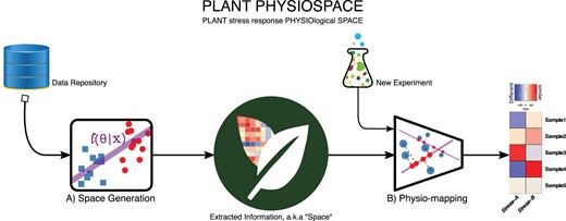
Plant PhysioSpace overview. The method consists of two main sections: space generation and Physio-mapping. A, In space generation, data from public repositories are processed and the relevant information is extracted. After trimming, the extracted information is stored in matrices called “space”, representing physiologically relevant expression patterns. B, Physio-mapping uses a space to analyze previously unknown data, for example, from another experiment. These data are mapped to the generated space, resulting in “similarity” scores that indicate the likeness of these data to the known physiological processes.
In this study, we focused on the application of our method in stress response analysis. As one of the fiercest adversaries of plants, biotic and abiotic stresses take a toll on commercial agriculture. Plant PhysioSpace can aid in engineering impervious crops by quantitatively analyzing the effect of a mutation or treatment on the plant’s resistance and/or tolerance.
Another long-lasting question in the field of stress response research is the potential heterogeneity in responses of cell types under stress. Generally, sequencing is done on thousands to millions of cells. This “average” look reveals only the mean effect on the bulk tissue, and lacks the direct assessment of individual cells. The unique role of different cell types shapes the function of their parent tissue; hence, by careful examination of stressed tissue cells, the differences between their behavior, and the interplay among them, one can gain insights into the complex mechanisms shaping the plant stress response.
Since 2009, more and more single-cell datasets are becoming available publicly. As with other recent technologies, the focus is mainly on human and animal tissue sequencing. Lack of data availability is especially true for plant studies since the presence of the cell wall has been a bothersome obstacle for single-cell technologies. But recent leaps in single-cell sequencing technologies, for example, the 10X platform, have resulted in the availability of a few plant single-cell datasets (Shulse et al., 2019; Denyer et al., 2019; Ryu et al., 2019; Jean-Baptiste et al., 2019; Zhang et al., 2019). Mostly, scRNA-seq studies follow the same analysis pipeline (Trapnell et al., 2014; Butler et al., 2018). In a nutshell, the highest variable genes are selected and analyzed through principal component analysis (PCA), followed by t-distributed stochastic neighborhood embedding (tSNE) or uniform manifold approximation and projection (UMAP), to demonstrate the underlying structure. Subsequently, clustering or regression algorithms are used to identify biologically relevant groups (e.g. groups of cells with a similar response), or trends (e.g. pseudotemporal axes of cell development), in the underlying data structure (Rich-Griffin et al., 2019). Though technologies such as 10X made plant single-cell sequencing possible, they are far from perfect. For instance, compared to bulk sequencing technologies, technical noise has a higher interference on single-cell reads, which calls for developing sophisticated bioinformatics analysis tools to handle those interferences.
This article is organized in the following way: it begins with the benchmarking section, in which the method’s performance is assessed by translating stress response among different experiments, platforms, and species. Benchmarking is followed by two application showcases in which we demonstrate two Plant PhysioSpace use-cases: investigating time-series data from biotic-stressed wheat, and analyzing a heat-stressed single-cell dataset. The article will then give a brief summary and critique of the findings in the “Discussion” section. Finally, a detailed explanation of the Plant PhysioSpace algorithm, encompassing both a review of the already published method and the modifications adapting the method to the field of plant stress research, is provided in the “Materials and methods”.
Results
Stress space verification by GO analysis
To validate our space generation process, we utilized the gene list analysis section of PANTHER (Thomas et al., 2006; Huaiyu Mi et al., 2019). We generated a model (i.e. a space) from Arabidopsis (Arabidopsis thaliana) microarray data called mean meta-stress space (explained in detail in “Materials and methods”). For each stress group in , we selected the genes with an absolute score value of more than one and a half (For BioMone and FeDeficiency stresses with cutoff of 1.5, ˂10 genes were selected, which is too small of a set for list enrichment analysis. Hence in these two cases, cutoff is reduced to one.), and tested this gene list by PANTHER overrepresentation test against gene ontology (GO) biological processes (Figure 2; Supplemental dataset S1; Supplemental Figures S1–S15). From 15 different stress groups, 11 were found to have the GO terms corresponding to the same stress enriched, with significant corrected P ˂0.001.
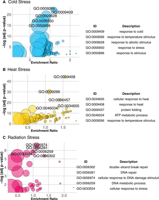
GO analysis of mean stress space. Results of GO analysis on three stress groups are demonstrated using bubble plots: cold stress (A), heat stress (B), and radiation stress (C). A–C, Each enriched GO term is represented by a circle, with adjusted P-values as y-axis and enrichment ratio as x-axis. The size of the circle shows the size of the gene list of the corresponding GO term. Enrichment ratio here means the ratio between the actual number of DEGs and the expected number in each GO group. For each plot, the five most significant GO terms are labeled on the plot and listed in a table beside each plot. Complete set of bubble plots and set of significant GO terms for all 15 stress groups are provided in Supplemental Figures S1–S15. Plots were generated using the GOplot package in R (Walter et al., 2015).
Inter-technology translation
Next-generation sequencing (NGS) has revolutionized the biological sciences. Its speed, cost, and data quality have outpaced the older DNA-microarray technology, which is why NGS became the standard method to study transcriptomes. Yet, microarrays were used for RNA quantification for decades. The vast microarray backlogs have the potential to grant an invaluable resource for future biological studies. Unfortunately, the measurement technology has an inevitable impact on the transcript measurement levels and the distribution of the resulting data. Data derived from different platforms are distinctly different. Hence, there are numerous methods to translate measurements from one technology to another (Love et al., 2014; Ritchie et al., 2015). Moreover, with the third-generation sequencing right around the corner (PacBio and Nanopore, to name a few (Niedringhaus et al., 2011)), there is a high demand for computational methods capable of transferring useful information between different measurement technologies.
Since PhysioSpace utilizes the differential expression relations of the genes and not the absolute values (see “Materials and methods”), it can translate between different measurement technologies. The translation success is contingent on the availability and accuracy of the method used for detecting the differentially expressed genes (DEGs) in the considered technology. To demonstrate the translation capabilities of Plant PhysioSpace, we mapped >900 RNA-seq samples into the microarray space (explained in detail in “Materials and methods”; Table 1). Our method could map the same stress type from microarray to RNA-seq data with 78% accuracy. We also calculated the probability of acquiring this accuracy by chance, by randomly permuting the sample labels and calculating the random accuracy. The performance of our method was significantly higher than any random accuracy we acquired (The highest acquired accuracy from 10,000,000 random runs for RNA2DNA translation was 52% (minimum = 12.08%, first quartile = 28.12%, median = 30.87%, third quartile = 33.56% and maximum = 52.35%).), with a P-value of ˂.
Stress translation between platforms and species
| Method | Measure | RNA-Seq to DNA-Array, Both Arabidopsis | Rice to Arabidopsis, Both DNA-Array | Soybean to Arabidopsis, Both DNA-Array | Wheat to Arabidopsis, Both DNA-Array |
|---|---|---|---|---|---|
| Plant PhysioSpace | Accuracy | 0.78 | 0.59 | 0.57 | 0.23 |
| P-value | 0.002 | ||||
| GSEA | Accuracy | ||||
| P-value | |||||
| Weighted Connectivity Score | Accuracy | ||||
| P-value | |||||
| Pearson Correlation | Accuracy | ||||
| P-value | |||||
| Spearman Correlation | Accuracy | ||||
| P-value | |||||
| Euclidean Distance | Accuracy | 0.39 | |||
| P-value |
In each column, the best performer is marked in bold.
Inter-species translation
Although not agriculturally relevant, Arabidopsis is arguably the most investigated species in plant sciences. Its availability, compact size, and fast growth make it an ideal model species. However, there are substantial differences between the Arabidopsis plant model and crop plants. These dissimilarities necessitate procedures for converting well-studied physiological knowledge from Arabidopsis to crops, for example, regarding plant response to different types of stress. In this section, we show how Plant PhysioSpace can be utilized for this purpose.
We chose three of the most commercially relevant crops to study: rice (Oryza sativa), soybean (Glycine max), and wheat (Triticum aestivum). For each crop, >100 microarray samples of stress response experiments were curated, normalized, preprocessed, and mapped to the Arabidopsis space . For rice and soybean, Plant PhysioSpace achieved respective accuracies of 59% and 57%, both of which were significantly higher than any accuracy earned by chance. On the other hand, translation of stress response from wheat DNA array data to Arabidopsis, with an accuracy of 23% and a P-value of 0.015, was not successful (Table 1). In “In-depth investigation of wheat stress response” section of this article, we provide a thorough investigation into wheat to Arabidopsis translation, hypothesize, and examine the reason behind the translation failure, and provide solutions for fixing it.
Benchmarking Plant PhysioSpace against other methods
We used the results from inter-technology and inter-species stress response translation to benchmark our method. Plant PhysioSpace is compared to common approaches used in bioinformatics for measuring relations between two or more gene expression samples: Gene Set Enrichment Analysis (GSEA) (Lamb et al., 2006); Weighted Connectivity Score, which is an advanced version of GSEA used in connectivity map (Subramanian et al., 2017); Pearson and Spearman correlations; and Euclidean distance. For each method, fold change values of samples, from different technologies and species, were calculated and used for finding the similarities between samples. Based on our results in inter-species and inter-platform mapping, Plant PhysioSpace could outperform other methods in all scenarios except in mapping from wheat to Arabidopsis (Table 1).
In-depth investigation of wheat stress response
As mentioned before, our method had a poor performance in translating stress response from wheat to Arabidopsis. The failed translation potentially stems from the microarray used to measure the wheat gene expressions. All microarray samples of wheat in this study are generated using Affymetrix Wheat Genome Array (https://www.ncbi.nlm.nih.gov/geo/query/acc.cgi?acc=GPL3802). Therefore, the aged technology could potentially deter the accuracy of transcription measurements. In addition, as a polyploid, the complex genetics of wheat makes the task of measuring its RNA levels troublesome.
Moreover, among all translations tested, wheat microarray data provide the least amount of mapped putative orthologs. In translating between different species, we utilize putative orthologs (explained in detail in “Materials and methods”). When translating from RNA-seq to microarray Arabidopsis stress data, we could find 12,146 common features (i.e. genes). This amount was lower for both translations of rice and of soybean to Arabidopsis, as the putative ortholog mapping could find 9,455 and 9,452 common features for them, respectively. And, in translation from wheat to Arabidopsis, 6,202 common features could be found using the putative ortholog mapping, which is the least among the four translations. These common feature counts correspond to the translation performance, considering the RNA-seq to DNA-microarray has the highest and wheat to Arabidopsis has the lowest accuracy, while rice and soybean mappings are somewhere in between (Table 1). This relationship suggests that a possible reason behind the failed wheat translation is the low number of putative orthologs.
Fortunately, advances in NGS gave rise to wheat stress response datasets with higher precision and a wider range of sequence reads. In this section, we repeated the wheat-to-Arabidopsis translation from inter-species analysis, except with wheat RNA-seq instead of microarray data. We turned to the Wheat Expression Browser (Borrill et al., 2016; Ramirez-Gonzalez et al., 2018) as the source of wheat RNA-seq data. From this source, we queried all datasets that study stress response, contain >30 samples, and include controls. Upon the first inspection, 8,813 putative orthologs could be found between these datasets and the genes available in our Arabidopsis reference space. The higher number of available putative orthologs, in addition to the improved data quality provided by RNA-seq, increases the prospect of Plant PhysioSpace correctly detecting and quantifying the stress in these datasets. We mapped these datasets into mean meta-reference space , and plotted physio scores of the three stress groups with the highest values (Figure 3).
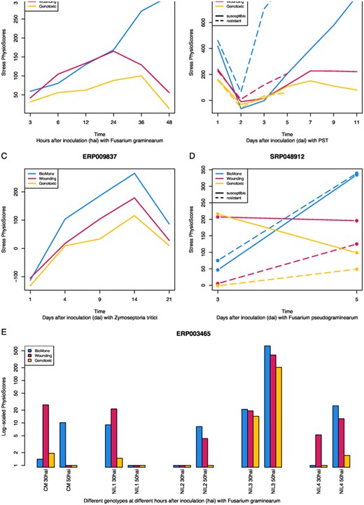
Time series analysis of biotic stress response of wheat RNA-seq data. Five different biotic-stressed datasets from Wheat Expression Browser are mapped to the Arabidopsis space , and the three groups with highest stress values are plotted for each dataset. A, Wheat response after inoculation with fungal pathogen F. graminearum is measured through time. B, Responses of two different MTs of wheat are studied to wheat yellow rust pathogen PST. C, Plants went through the infection cycle of the hemibiotrophic fungus Z. tritici. D, The responses of two different traits of resistant and susceptible wheat to Fusarium crown rot are studied. E, Behavior of five different genotypes under the disease pressure of F. graminearum is studied. The five investigated genotypes consist of CM-82036 (CM), a progeny of the resistant Sumai-3, and four NILs bearing either one, both, or none of the resistant alleles Qfhs.ndsu-3BS (also known as Qfhb1 or Fhb1) and Qfhs.ifa-5A. Among the four, NIL1 is a MT with both QTLs, expected to have the highest resistance after CM-82036. NIL2 and NIL3 are MTs harboring Fhb1 and Qfhs.ifa-5A QTL, respectively, with both predicted to behave moderately resistant. NIL4 lacks both QTLs, and is likely to be susceptible. In four out of five cases, BioMone stress group has the highest similarity value, with resistant MTs having higher responses than the susceptible ones (A–D). This figure is generated using ggplot2 package (Wickham, 2016).
In the experiment set ERP013829, wheat response after inoculation with fungal pathogen Fusarium graminearum is measured through time (Schweiger et al., 2016). For this experiment, Plant PhysioSpace correctly predicts that wheat is experiencing Biotic and Hormone (BioMone) stress. In addition, the diachronic rise in the response indicates how physio scores are quantitatively comparable (Figure 3).
In the dataset ERP013983, responses to wheat yellow rust pathogen Puccinia striiformis f.sp. tritici (PST) are studied in two different mutants (MTs) of wheat. The authors focused on the pathogen suppression of basal defense in plants (Dobon et al., 2016). From their results, they deduced that the pathogen overcame the defense by rapidly suppressing the genes involved in chitin perception on Day 2 after inoculation. In the susceptible interaction, this provides the possibility for the invasion and colonization, while in resistant plants, this suppression is quickly averted. Plant PhysioSpace results reflect this mechanism correctly: both plant types are reacting with a BioMone response on Day 1, followed by a suppression of the plant defense response on Day 2. Eventually, the quick resurgence of intense BioMone response in resistant wheat helps it in withstanding PST, while the reaction of the susceptible trait might be too slow to deflect the pathogen (Figure 3).
Plants in ERP009837 went through the infection cycle of the hemibiotrophic fungus Zymoseptoria tritici. Similar to ERP013829, plants respond to the pathogen with a dominant BioMone response (Figure 3). Yet, unlike ERP013829, in which the experiment spanned a few hours, in ERP009837, plants were studied for a longer period. Physio scores suggest that wheat responds to the presence of the pathogen by increasing its BioMone response. This response starts to degrade from Day 14, which is in alignment with the original publication of the dataset (Rudd et al., 2015). That is because in the original publication, the authors reported about the degradation of the plants near the end of the timeline and stated that plant tissue was completely defeated on Day 21.
In SRP048912, the responses of two different traits of resistant and susceptible wheat to Fusarium crown rot are studied (Ma et al., 2014). Only two different time points are included in this experiment: 3 and 5 d after inoculation. Plant PhysioSpace results correctly suggest that the most dominant stress response present in plants is BioMone, with the resistant wheat having a stronger response than the susceptible wheat (Figure 3).
Among the wheat datasets we analyzed in this section, ERP003465 is arguably the most complex, and consequently, most interesting as a testing scenario for our method. In ERP003465, they examined the behavior of five different genotypes under the disease pressure of F. graminearum (Kugler et al., 2013). Two well-validated and highly reproducible quantitative trait loci (QTLs), Qfhs.ndsu-3BS (syn. Qfhb1 or Fhb1) and Qfhs.ifa-5A, are studied in samples taken 30 and 50 hours after inoculation (hai). Five different genotypes were investigated: CM-82036, a progeny of the resistant Sumai-3, and four near-isogenic lines (NILs) bearing either one, both, or none of the resistant alleles Fhb1 and Qfhs.ifa-5A. Among the four, NIL1 is an MT with both QTLs, expected to have the highest resistance after CM-82036, NIL2 and NIL3 are MTs harboring Fhb1 and Qfhs.ifa-5A QTLs, respectively, with both predicted to behave moderately resistant, and NIL4, which is missing both QTLs, is likely to be susceptible.
Data analysis in the original paper was mainly based on differential expression analysis. As a first step, the total number of DEGs for each genotype at each time point was calculated. This total number was taken as a surrogate for stress response intensity in each genotype at each time point. In the next steps, the weighted gene co-expression network analysis was used to detect clusters of genes with similar patterns, and GO term enrichment analysis was utilized to infer the role of each cluster in the stress response.
Being able to quantify the intensity of each stress type at each time point, Plant PhysioSpace can provide much more insight into the characteristics and dynamics of the stress responses that are at play in the ERP003465 experiment (Figure 3). As this dataset encompasses a high number of samples distributed between only two time points, we plotted the results as a bar graph. And because the results cover a wide range of values for this experiment, we used log-scaled physio scores in the graph, and replaced values smaller than one with one (zero in log-scale).
Among the concluding remarks in the original paper, some are in concordance with the results from our method. For example, lines lacking Qfhs.ifa-5A are regarded as “slow responders” by the original authors, since these lack resistance against initial infection inferred by Qfhs.ifa-5A. This lack of early response can be seen in our results (Figure 3): lines lacking Qfhs.ifa-5A, that is, NIL2 and NIL4, have no BioMone stress response at the early time point, while NIL1 and NIL3 show a considerable BioMone stress response at the same time point. Another remark from the original paper suggests that a lack of timely defensive reaction could result in a higher infection at a later time, and consequently, a stronger response. The reverse could potentially be true as well: a quick response may reduce the response intensity and infection at a later time. This can be seen in the contrasting response dynamics of NIL1 versus the other lines (Figure 3). NIL1 possesses both QTLs; Qfhs.ifa-5A ensures an early and fast stress response, evident at the 30 hai time point. And a strong follow-up, courtesy of Fhb1, results in a nonexistent BioMone response at 50 hai. NIL3 contains Qfhs.ifa-5A, so it benefits from a quick response at 30 hai. However, due to the absence of Fhb1, this line (i.e. NIL3) cannot be rid of infection at 50 hai, evident by the high BioMone response at that time point. As mentioned, lines NIL2 and NIL4, which lack Qfhs.ifa-5A, do not have an early response and have to play catch up with other lines at the later time point.
Although many conclusions that could be derived from our method are similar to the ones from the original publication, there are some discrepancies between the two groups as well. For instance, Wounding stress response is not only present in most samples, but it is even stronger than BioMone response in some cases. This is in contrast with the original paper, in which it is mentioned that inoculation was done cautiously without wounding the tissue. Interpretation of CM-82036defensive behavior is another point of difference between our method and the results from the original paper. Kugler et al. construed the high number of DEG at 30 hai as a sign of strong early response for CM-82036, even stronger than NIL1 and NIL3. They followed up by studying specific gene families that are relevant to defense mechanisms, such as UDP-glycosyltransferase gene families and WRKY transcription factors, and showed more DEGs from these families can be found at 30 hai in CM-82036 versus in other lines. This finding is different from what we can interpret using our method: though CM-82036 exhibits BioMone response at 30 hai, the magnitude is somewhere between fast responder lines, that is NIL1 and NIL3, and slow responders, that is, NIL2 and NIL4.
We speculate the main reason for the aforementioned inconsistencies is the particular way the preprocessing was done in the original paper. In their preprocessing, Kugler et al. mapped the reads to a list of barley (Hordeum vulgare) high confidence genes and only used the reads with a possible match. This step drastically reduces the number of available transcripts, and also discards wheat-specific genes with no barley homologs. Our method is designed for high-dimensional data, preferably data from the whole genome. The specific preprocessing of this dataset, therefore, might have reduced the performance of Plant PhysioSpace. We should also mention that stress responses are not mutually exclusive; a plant can display multiple different responses at the same time, some of which may even share part of their biological pathways. Fusarium graminearum could have damaged the plant tissue at some point, which explains the existence of wounding response alongside BioMone.
Despite the mediocre results of the last experiment, in this section we showed how, in four out of five datasets, Plant PhysioSpace could:
Correctly identify the type of stress plants are going through.
Accurately relate the response from RNA-seq test data to DNA-array trained models.
Properly translate wheat stress response to Arabidopsis.
Plant PhysioSpace application in single-cell analysis
Single-cell technologies facilitate investigating transcription profiles at a single-cell resolution in order to perceive the genetic basis of each cell type and its function. Although relatively recent, an increasing number of plant single-cell datasets are becoming available to the community (Shulse et al., 2019; Denyer et al., 2019; Ryu et al., 2019; Jean-Baptiste et al., 2019; Zhang et al., 2019). For now, most sequence datasets are focused on Arabidopsis roots. These try to gain an in-depth understanding of transcription patterns of different cells in different developmental stages of WT nonstressed plant roots. To our knowledge, the only publication in which stressed single cells were sequenced is the paper by Jean-Baptiste et al. (2019). In this work, 38°C heat stress was applied to 8-d-old seedlings for 45 min. Subsequently, roots of the seedlings were harvested, along with the roots of age- and time-matched control seedlings. The authors could capture and sequence 1,009 cells from the stressed group and 1,076 from the control group. For processing the sequencing results, they followed the usual single-cell analysis pipeline: PCA, UMAP, and clustering, followed by differential gene expression analysis on clusters and enrichment tests on genes related to heat-shock. The results show the “promise and challenges inherent in comparing single-cell data across different conditions and treatments.” In this section, we demonstrate how a dedicated method, such as Plant PhysioSpace, can help in tackling the single-cell analysis challenges and provide additional benefits compared to the methodological norms.
To analyze the single-cell dataset, we used the gene-wise mean value of all control cells as the baseline, calculated fold changes for every single cell, and fed those fold change values into the Plant PhysioSpace pipeline. Regardless of the cell type, heat-stressed single cells had significantly higher heat stress scores compared to the control single cells (Figure 4). For studying the heat-induced cell type disparity, we overlaid heat stress scores on UMAP and tSNE plots (Figure 4). In both tSNE and UMAP plots, coordinate values calculated in the original paper of Jean-Baptiste et al. were used. As a result, cells are bundled in cell-type clusters in the UMAP plot. In the tSNE plot, however, cells are clearly separated into two big clusters of control and stressed, and sub-clusters of different cell types are evident inside these two big clusters (Supplemental Figure S16). On the UMAP plot on the other hand, big clusters represent cell types (Supplemental Figure S17). Inside each cell type cluster, groups of control and stressed cells may or may not be distinct. For example, in Hair and Nonhair clusters, control and heated cells are separated, while the separation is less pronounced in Stele cells (Supplemental Figure S17).
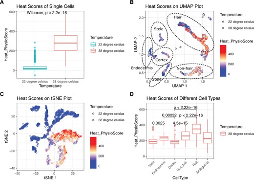
Single-cell analysis results of Plant PhysioSpace. Stress scores were calculated for each cell. A, For demonstrating the outcome, we plotted the heat score of the two big groups of control and stressed. This box plot proves how Plant PhysioSpace could correctly detect and quantify stress response in single-cell data. B and C, We overlaid the heat scores on UMAP and tSNE plots, respectively. D, Boxplot of heat scores, on y-axis, was plotted against different cell types, on x-axis. Cell types on the x-axis are ordered based on the morphological anatomy, starting from inner cell types to outermost cell layers (excluding Ambiguous cells, which come at the end). In the boxplots, Wilcoxon rank-sum test is used for statistical testing, the median is shown with a line inside each box, the lower and upper hinges correspond to the first and third quartiles, the upper whisker extends from the hinge to the largest value no further than from the hinge (where IQR is the inter-quartile range, or distance between the first and third quartiles), the lower whisker extends from the hinge to the smallest value at most of the hinge, and data beyond the end of the whiskers are plotted individually. This figure is generated using ggplot2 package (Wickham, 2016).
To look into the distinct behavior of different cells under stress, we also plotted cell heat scores grouped by the corresponding cell types (Figure 4; Supplemental Figure S18). The results show how Hair and Nonhair cells have higher heat scores, which demonstrates how the outer layers of roots are more precise in their response to heat. This finding is in concordance with one of the conclusions in the original paper, in which, based on the behavior of the heat-relevant genes, they concluded the three outermost cell layers of the root went through higher levels of changes caused by the heat stress. The authors hypothesized this may be because of the more direct exposure of the outer layers to the heat shock, resulting in a quicker and stronger response.
Although resulting in generally the same conclusions, in single-cell stress analysis, Plant PhysioSpace provided an advantageous experience for the end-user by providing:
Convenience: unlike the original paper, there was no need for search and curation of heat stress gene clusters, as they are already available in Plant PhysioSpace, as well as clusters for other common stresses.
Precision: not only the stress type but also the magnitude of the stress response could be quantified by our method, something which is lacking in traditional gene list enrichment approaches. For example, Plant PhysioSpace results suggest a stronger response in the Hair cells, compared to the Nonhair response (Figure 4). This inference could not be concluded from the results of traditional methods.
Optimization: in one run, our tool calculated responses of 20 different stresses for 2,085 single cells in ˂3 min on a 2-core laptop CPU. This swift performance is accomplished by precalculating the stress space, in combination with an optimized mapping algorithm, all of which is readily available for the community to use.
Availability
To provide the community with an easy-to-use implementation of our method, we built Plant PhysioSpace into two different R packages: a method package (https://git.rwth-aachen.de/jrc-combine/PhysioSpaceMethods) containing functions for generating new spaces and Physio-mapping, and a data package (https://git.rwth-aachen.de/jrc-combine/PlantPhysioSpace) comprising plant stress spaces such as and that were used in this paper.
In addition, we made a Shiny (http://shiny.rstudio.com) web application of Plant PhysioSpace (Figure 5). We hosted the web app on shinyapp.io (http://physiospace.shinyapps.io/plant/), to be freely available to use (under the terms of GPL-3 license). We also built a Docker image of the ready-to-use tool (https://github.com/usadellab/physiospace_shiny).

Plant PhysioSpace Web-application, with the address http://physiospace.shinyapps.io/plant/. A, Home page of the web-app. B, Results of a mock example analysis on the Plant PhysioSpace web-app.
Discussion
Gaining proper insight into stress response mechanisms in plants is not only a must for the future of agricultural research, but will prompt advances in the plant research field in general. In this article, we developed an advanced computational method for analyzing stress responses in plants. The lightweight algorithm allows the method to be run on personal computers or as a web application, making it an ideal tool for quality control, dataset annotation, to draw conclusions considering thousands of genes, and so on.
We built this method upon a previously published method in humans, called PhysioSpace. We adapted the method by curating a multitude of Arabidopsis stress response samples to have a rich training dataset. Additionally, we modified the space generation algorithm, that is, training, to acclimate to the specific characteristics of stress response data in plants. At the end, we thoroughly tested our method on different species and types of data. The results of this study demonstrated that Plant PhysioSpace can be a convenient and practical tool for analyzing stress response datasets, to comprehend, contrast to state of the art methods, or for quality control.
Notably, our tool could perform adequately even when it was mapping information between different platforms and species. Still, it is crucial to bear in mind that these cross translations necessitate some conditions. In cross-platform translation, it was assumed that with the same experimental setup and samples, there are computational pipelines that roughly compute the same DEG lists regardless of the platform used. And in cross-species mapping, we assumed putatively orthologous genes to have the same biological functions across all species; evidently, it is impossible for this assumption to be consistently true for all genes, but a sizable portion of genes have to pass this criterion for the inter-species translation to work.
Recent advances in single-cell technology call for suitable bioinformatics analysis tools (Rich-Griffin et al., 2019). We demonstrated how Plant Physiospace can provide insights when used for analyzing single-cell datasets. The provided benefits in single-cell data analysis bring a spectrum of applications to mind for the future, especially in the light of approaching plant single-cell atlas projects (Petryszak et al., 2016; Rhee et al., 2019).
Plant PhysioSpace may seem paradoxical at first, as it is explained to be a “dimension reduction” method that extracts stress information from gene expression data “without reducing dimensions.” Yet, this seemingly contradictory approach is possible since our method does not “a priori” reduce any dimension; Plant PhysioSpace does not discard any features from the training data when extracting stress information in the space generation stage (i.e. model training), but only removes the irrelevant features in the physio-mapping (i.e. when applying the method to the newly acquired samples). As mentioned before, the majority of genes remain unaltered under stress. We can show this unvarying behavior using the (Figure 6). Taking the absolute fold change value of 1 as a cutoff, only a small portion of plant genes are changing under stress. To be more specific, from all 22,249 genes available in , only 2,905 (∼13%) change under at least one stress type. In addition, the number of changed genes is a function of the stress type, ranging from ∼0.07% in BioMone (biotic, hormone, or both stresses) to ∼5.8% in the Drought.Light (double stress) group (Figure 6). Moreover, the majority of varying genes are specific to a stress group, as 2,175 out of the 2,905 genes (∼75%) only change in one stress group (Figure 6). The low dimensionality of the stress responses, along with the high specificity of the features, may suggest that one can remove the genes with the absolute fold change of ˂1 in the training step. It may seem that keeping all the features till the end is not beneficial, while removing them could result in an even more compressed model. We are against this exclusion, however, on the ground that the removal of genes with an absolute fold change of ˂1 can eliminate relevant information. As proof, we ran the single-cell analysis of the last section once more using a “reduced” , which is a version of , with all the 2,905 varying genes removed (Figure 6). Though not as high as their counterparts calculated by using the complete , heat scores calculated using the reduced space are still significantly higher in heated single cells compared to the control cells (Wilcoxon rank-sum test P-value ). These results prove that the genes with less varying expression also carry stress-related information. Therefore, we conclude the benefits of keeping all possible features outweigh the advantages that come about by removing them. Having the information from the whole genome at hand is especially helpful when analyzing datasets that do not include a high number of genes because the overlap between the features present in both the model and the newly acquired dataset may become too small. Many single-cell sequencing technologies, such as the Oxford Nanopore MinION (Jain et al., 2016), provide readings on a limited number of genes, and keeping the whole genome in the trained model can boost the performance of our method on data from the aforementioned technologies. That being said, a proper and clever way of reducing dimensions of the trained spaces has the potential to increase the efficiency and reduce the complexity of our method.
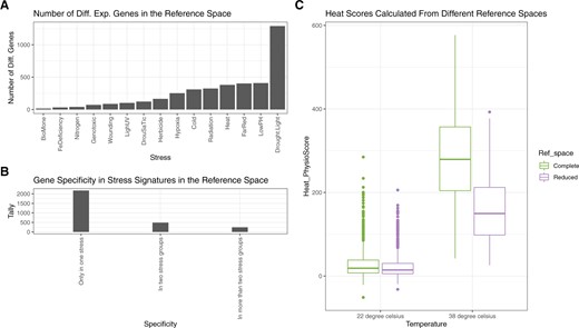
DEGs in the , their specificity, and their effects on the performance of Plant PhysioSpace. A, The number of genes with an absolute fold change value of >1 in each stress group is demonstrated. Since there are 22,249 genes available in the space , the ratio of DEGs to all genes among different stress groups spans from around 0.07% in BioMone (biotic, hormone, or both stresses) to around 5.8% in the Drought.Light (double stress) group. B, We explored the specificity of DEGs to stress groups. Among all 22,249 genes in , only 2,905 (∼13%) are differentially expressed in one or more stress groups. From these 2,905 genes, 2,175 (∼10%) are specifically expressed in only one stress group, 488 (∼2%) are expressed in two stress groups, and 242 (∼1%) in more than two stress groups. Hence, we conclude that the majority of expressed genes in the are specific to one stress group. C, We used the heated single cells to study the effect of the 2,905 DEGs on applicability of as a reference. We compared the performance of against without the 2,905 DEGs, which we called the “reduced” . As evident from the boxplot, the heat scores are still substantially different between control and heated cells, even when the reduced space is used, although the magnitude of the heat scores is decreased compared to when the complete space is used. In the boxplot, the median is shown with a line inside each box, the lower and upper hinges correspond to the first and third quartiles, the upper whisker extends from the hinge to the largest value no further than from the hinge (or distance between the first and third quartiles), the lower whisker extends from the hinge to the smallest value at most of the hinge, and data beyond the end of the whiskers are plotted individually. This figure is generated using ggplot2 package (Wickham, 2016).
To our knowledge, Plant PhysioSpace is the only computational tool available that is capable of quantitizing stress response in plant cells. Therefore, it can be used to assess each cell under stress, to grasp an understanding of the complex responses and interplay of cells in plants under stress, and to achieve a comprehensive characterization of plant response to stress overall.
Materials and methods
Data preparation
While setting up a PhysioSpace matrix, our method requires extensive training data for achieving adequate robustness. This training data can be retrieved from retrospective datasets. To that end, we curated >4,000 plant stress response gene expression samples from Gene Expression Omnibus (GEO) (https://www.ncbi.nlm.nih.gov/geo/) and Sequence Read Archive (SRA) (https://www.ncbi.nlm.nih.gov/sra/). More specifically, 2,480 Arabidopsis array samples, 967 Arabidopsis RNA-seq samples, 146 rice array samples, 172 soybean array samples, and 104 wheat array samples were used for space generation. Each sample is annotated with a label from a stress set. In this study, samples are divided into Aluminum, Magnesium, Biotic, Cold, Drought, FarRed, FeDeficiency, Genotoxic, Heat, Herbicide, Hormone, Hypoxia, Light, LowPH, Metabolic, Mutant, Nitrogen, Osmotic, Radiation, Salt, Submergence, UV, and Wounding stress groups. For samples that underwent more than one stress, new labels were generated by concatenating existing labels from the stress set. For example, “Biotic.Drought” designates a sample that sustained both Biotic and Drought stresses.
Samples corresponding to each species are normalized in bulk to remove the batch effects. We used robust multi‐array average (Irizarry et al., 2003) for normalizing microarray RAW data files, and a pipeline consisting of Fastq-dump, Trimmomatic (Bolger et al., 2014), Star aligner (Dobin et al., 2013), and featureCounts (Liao et al., 2014) to derive counts from SRA records.
PhysioSpace method
PhysioSpace is a supervised dimension reduction method, which aims to extract relevant physiological information from big datasets and store it in a mathematical space (Lenz et al., 2013). The method can be divided into two main steps: space generation and physio-mapping (Figure 7).
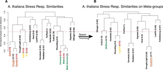
Space trimming. A, Stress groups are clustered and for each group, LOOCV accuracy is calculated, written in parenthesis. Clustering is done using physio scores; physio scores are normalized using min–max normalization (values are rescaled to span from 0 to 1), and since physio score is a measure of similarity, are used as the distance measure for clustering. Y-axis represents this distance measure. B, Close groups with low accuracy, written in red, are combined to form new stress groups, called meta-groups. Groups are considered close if they merge in the dendrogram in a height ˂0.5 (50% of maximum height). This cut-off height is shown in the figure with a dashed red line. In this figure, Salt, Drought, and Osmotic stress groups, marked with underlined text and brown color, merge into DrouSaTic meta-group; Hormone, Biotic, and Biotic.Hormone groups form BioMone meta-group, written in green with italic font, and Light and UV groups combine into LighUV, shown in light yellow.
Space generation
After preparing the data, we derive the physiologically relevant information from normalized data and store this information in a mathematical space. This step is comparable to training in machine learning terminology. Space generation is done in two stages: space extraction and space trimming. The former stage is identical to the method described previously in (Lenz et al., 2013). However, space trimming is an innovative addition to adapt the method for studying plant stress response.
Space extraction
In the PhysioSpace method, all samples are analyzed contrastively, that is, using differential expression analysis. “Space” is a matrix that is built upon reference data. In this article, reference data contain all Arabidopsis array samples that are measured by the Affymetrix Arabidopsis ATH1 Genome Array (https://www.ncbi.nlm.nih.gov/geo/query/acc.cgi?acc=GPL198). For each stress group in each dataset, gene-wise fold changes are calculated between stressed plants and their corresponding controls. The fold changes fill one column of the space matrix. This generated matrix, which we call , contains the stress-relevant information represented in the reference data. In addition to , we calculated the mean reference space(). For constructing , for each stress group, the gene-wise mean value of fold changes in are calculated and stored in a column in . More detailed information, as well as a step-by-step guide for creating and , are provided in Supplemental text S1.
Space trimming
The stress grouping in this study is done based on the expert annotation provided alongside public datasets. Therefore, this grouping does not necessarily reflect the different classes of biological mechanisms that shape the plant response spectrum. There are different groups of biologically related stresses, and stresses in the same group have similar stress response signatures. For instance, stresses to which plants respond using the same common mechanisms and pathways have similar gene expression fingerprints. On the other hand, stresses have substantially different gene expression patterns when few to no common genes are involved in their corresponding stress responses.
From the mathematical point of view, the similarity between distinct stress responses manifests itself in the collinearity of axes in the extracted space. Collinearity in a mathematical space is a source of redundancy, and in our application, can result in lower accuracy and robustness.
We came up with an algorithm named space trimming: an unsupervised approach that in combination with space extraction, makes up a hybrid method that can detect previously undetected groups of stress responses. We call these new-found groups meta-stress groups. Space trimming uses a consecutive combination of hierarchical clustering and leave-one-out cross-validation (LOOCV) to remove the aforementioned redundancy from a space. Space trimming consists of three steps:
Clustering and cross-validation analyses are done on the space under study, and a dendrogram based on the calculated similarities is constructed.
In the dendrogram, groups of stresses that are adjacent and have low accuracy are combined to make meta-stress groups. Groups that merge under 50% of the maximum height in the dendrogram (i.e. groups with the distance of 50% of the maximum distance or lower) are considered close, and groups of stresses that have an accuracy of ˂0.7 are considered low in accuracy.
Any newly generated meta group that has at least the same performance as its subgroups is kept. All other meta groups are reverted back to their former groups.
We applied the space trimming algorithm to the , the Arabidopsis microarray space we generated in the last section (Figure 7).
In LOOCV, by definition, one sample is left out for testing. In our LOOCV scheme, however, we left out one GSE (GEO (https://www.ncbi.nlm.nih.gov/geo/) Series) dataset in each cycle. Due to batch effects, even with proper preprocessing, samples from the same GSE set tend to be similar. With leave-one-GSE-out cross-validation, we make sure that the stress response from different datasets could be successfully matched together.
In each iteration, one GSE dataset is chosen as the test set, it is mapped to the rest of the datasets (i.e. the training set), and it is counted as a successful match if the analyzed test data and its most similar dataset from training set fall under the same stress group. Using the confusionMatrix function from the caret package (Max Kuhn, 2020) in R, matching accuracy and robustness of the method are evaluated (Figure 7). With an overall balanced accuracy of , a Cohen’s kappa of , and an accuracy P-value of , PhysioSpace could successfully match the samples going through the same stress group.
As expected, clustering analysis exposed the similarities among different stress responses. For instance, responses to Osmotic, Drought, and Salt stresses seem to have common underlying activated gene groups. Or regarding Biotic, Hormone, and Biotic.Hormone (double stress), their close proximity points toward a very similar stress response. They also predominantly have lower accuracy compared to other stress groups (Figure 7). This led us to the assumption that these groups of stress responses share one or few underlying defensive mechanisms, such as an innate immune response.
Merging the similar stress groups and constructing the meta-stress groups result in an improved performance of the method (Figure 7). We constructed three new meta-stress groups: BioMone, which is composed of Biotic, Hormone, and Biotic.Hormone stress groups; DrouSaTic, that was built by combining Drought, Salt, and Osmotic stresses; and LighUV, which is made by merging Light and UV stresses (Figure 7). Redoing the LOOCV on the newly acquired space (i.e. the space containing the meta-stress groups) demonstrates the performance gain, with an accuracy of 0.57 and a Cohen’s kappa of 0.49. Compared to the classical grouping of stresses, the new performance shows an increase of 0.14 and 0.105 in the accuracy and Cohen’s kappa, respectively. The accuracy P-value stays significant, as it is equal to .
The resulting space, which we call , and its successive mean space which we denote by , are the spaces we use as references throughout the “Results”. But we should mention the possibility of using and , or any other reference that could be generated using the algorithms in this section. For example, in a case where individual Salt and Drought stresses are needed to be characterized and quantified, can be utilized in place of .
Physio-mapping
After acquiring a space from known training data, we can map data from any technology or species back into the space and find similarities between the unknown input and the known training data. Physio-mapping is a nonlinear, model-free mapping, designed to take advantage of omics data structures and to compensate biases from heterogeneous assessment protocols. Omics are mostly framed in high-feature low-sample arrangements. In most cases, the majority of features in these types of datasets are intrinsically dominated by noise rather than physiologically informative facts about the samples under study. Results commonly acquired by differential expression analysis are great demonstrators of this phenomenon; in most cases, only a small proportion of features in an omics dataset is significantly different. In other words, only a small portion of features corresponds to circumstances that are being studied.
Considering the unique omics characteristics, our proposed mapping is done by taking the following steps:
Either
A new space is extracted from the new data. This means that for each gene in each stress case, a fold change is calculated by modeling the gene behavior under the respective stress given the control. We call this new input space .
For each stress type , genes are sorted from the lowest to highest fold change.
percent lowest and highest genes are selected as and for each . is a user-defined parameter. In this paper, it is between 3% and 5%.
or
(2) For each axis in the reference (e.g. each column in ), a statistical test is performed between and gene groups to form the matrix:
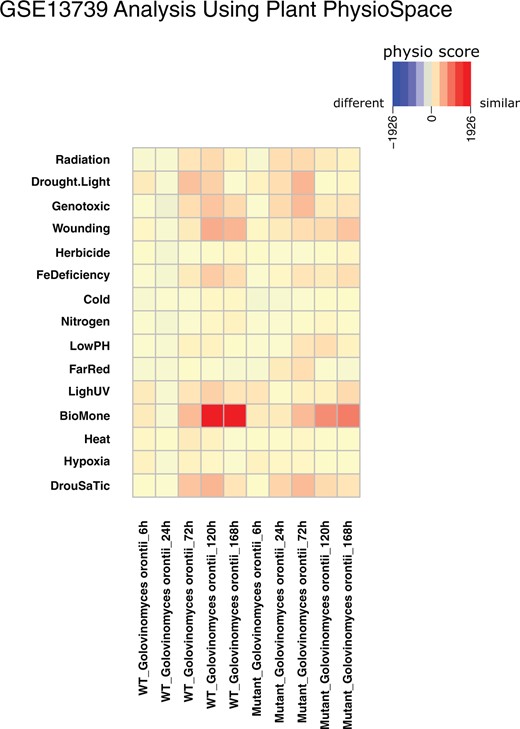
Analysis results of GSE13739. The GEO dataset GSE13739 is mapped against using Plant PhysioSpace. The dataset provides samples of WT and MT Arabidopsis plants that are infected with G. orontii (Biotic stress). The MT plants are expected to be more resilient.
For inter-species mapping, for instance, in analyzing data from rice using a space generated from Arabidopsis, we resorted to putatively orthologous genes. By using the ideal assumption of putative orthologs having identical biological roles in all species, we mapped genes to their putative orthologs in cases with inter-species translation. For the mapping, we utilized the Basic Local Alignment Search Tool BLAST (Boratyn et al., 2013). More specifically, we used the BLASTn tool to align sequences from rice, soybean, and wheat against Arabidopsis, with as the cutoff for the “expect value.” Expect value, also known as expectation value or e-value, represents the number of random alignments with scores equivalent to or better than the resulted match (Bergman, 2007). In other words, the expected value depicts the statistical significance of the alignment. Therefore, to have a one-to-one match between genes from different species and Arabidopsis, the gene with the lowest expected value is chosen in cases with multiple possible matches.
Accession numbers
Sequence data of the major genes/proteins mentioned in this article can be found in the GenBank data libraries under accession numbers_JN696291.1 (FvC5SD), KX907434.1 (Fhb1), and JX624788.1 (Qfhs.ifa-5A). Accession numbers of gene expression datasets used in this article can be found in the documentation of our data package.
Supplemental data
The following materials are available in the online version of this article.
Supplemental Dataset S1. GO Analysis results of the .
Supplemental Figures S1–S15. GO analysis resulting figures of the .
Supplemental Figures S16–S18. Single-cell analysis results of Plant PhysioSpace.
Supplemental Text S1. Space extraction in detail.
Funding
This work was partially funded by Bayer AG. In addition, B.U. was partially supported by the Deutsche Forschungsgemeinschaft (through the DFG project CEPLAS EXC 390686111).
Data availability statement
All the scripts that generate the results of this paper can be found in https://git.rwth-aachen.de/jrc-combine/PlantPhysioSpacePaper.
Conflict of interest statement. The authors of this manuscript declare no competing financial interests. The funders of this manuscript, listed in the funding section, had no role in study design, method development, data collection and analysis, decision to publish, or preparation of the manuscript.
B.M.S. and A.S. conceived the original method and research plans; B.M.S. and D.N. implemented an earlier version; A.S. supervised the method development and calculations; A.H.E. designed the improved method and analyzed the data; B.M.S. conceived and analyzed a preliminary version of the single-cell section; A.H. implemented the web-app; D.N., J.M., A.H., M.O., B.U., and B.B. provided technical assistance to A.H.E.; A.H.E. conceived the project and wrote the article with contributions from all the authors; A.S., A.H., B.B., M.O., B.U., and B.M.S supervised and completed the writing. A.S. agrees to serve as the author responsible for contact and ensures communication.
The author responsible for distribution of materials integral to the findings presented in this article in accordance with the policy described in the Instructions for Authors (https://dbpia.nl.go.kr/plphys/pages/general-instructions) is: Andreas Schuppert ([email protected]).
References
Author notes
Senior author.
