


Abstract
Dissecting the genetic basis of complex traits is aided by frequent and nondestructive measurements. Advances in range imaging technologies enable the rapid acquisition of three-dimensional (3D) data from an imaged scene. A depth camera was used to acquire images of sorghum (Sorghum bicolor), an important grain, forage, and bioenergy crop, at multiple developmental time points from a greenhouse-grown recombinant inbred line population. A semiautomated software pipeline was developed and used to generate segmented, 3D plant reconstructions from the images. Automated measurements made from 3D plant reconstructions identified quantitative trait loci for standard measures of shoot architecture, such as shoot height, leaf angle, and leaf length, and for novel composite traits, such as shoot compactness. The phenotypic variability associated with some of the quantitative trait loci displayed differences in temporal prevalence; for example, alleles closely linked with the sorghum Dwarf3 gene, an auxin transporter and pleiotropic regulator of both leaf inclination angle and shoot height, influence leaf angle prior to an effect on shoot height. Furthermore, variability in composite phenotypes that measure overall shoot architecture, such as shoot compactness, is regulated by loci underlying component phenotypes like leaf angle. As such, depth imaging is an economical and rapid method to acquire shoot architecture phenotypes in agriculturally important plants like sorghum to study the genetic basis of complex traits.
The rate-limiting step for crop improvement and for dissecting the genetic bases of agriculturally important traits has shifted from genotyping to phenotyping, creating what is referred to as the phenotyping bottleneck (Houle et al., 2010; Furbank and Tester, 2011). Alleviating the phenotyping bottleneck for agriculturally important plants will help the world meet the increasing food and energy demands of the growing global population (Somerville et al., 2010; Alexandratos and Bruinsma, 2012; Cobb et al., 2013). Approaches to alleviate the plant phenotyping bottleneck fall into two broad categories: approaches that increase the number of individuals that can be grown and evaluated (Fahlgren et al., 2015b) and approaches that predict performance in silico to prioritize individuals to grow and evaluate (Hammer et al., 2010; Technow et al., 2015). Both of these approaches will be instrumental for increasing the rate of crop improvement, and both approaches are facilitated by advances in image-based phenotyping; multiple plant measurements can be acquired rapidly from images, and data from image-based phenotyping approaches also can inform performance prediction (Spalding and Miller, 2013; Pound et al., 2014). As such, the development of image-based phenotyping platforms for agriculturally important plant species is a high priority for plant biology and crop improvement (Minervini et al., 2015).
The diversity of crop species and the variety of traits of interest have resulted in the development of a number of different platforms for plant phenotyping (Cobb et al., 2013; Li et al., 2014). Commercial platforms, including the Scanalyzer series from Lemnatec (http://www.lemnatec.com/products/; accessed February 2016) and the Traitmill platform from CropDesign (http://www.cropdesign.com/general.php; accessed February 2016), have gained adoption in the research community and have promoted the development of additional software (beyond that which the respective companies provide) to analyze the images produced by the platform (Reuzeau, 2007; Hartmann et al., 2011; Fahlgren et al., 2015a). A variety of noncommercial platforms and methods developed by the research community also exist and have been demonstrated to perform well (White et al., 2012; Fiorani and Schurr, 2013; Sirault et al., 2013; Pound et al., 2014). Several platforms have been deployed at sufficiently large scale to examine genomic loci underlying complex traits in crop plants such as barley (Hordeum vulgare; Honsdorf et al., 2014), pepper (Capsicum annuum; van der Heijden et al., 2012), maize (Zea mays; Liu et al., 2011), rice (Oryza sativa; Campbell et al., 2015), and wheat (Triticum aestivum; Rasheed et al., 2014). These successful applications of image-based phenotyping to understand the genetic bases of complex crop traits represent only a small fraction of the imaging modalities and crop species available for study. Sorghum (Sorghum bicolor) is the fifth most produced cereal crop in the world and is a promising bioenergy feedstock (Mullet et al., 2014). Recent work has demonstrated that optimization of plant canopy architecture has the potential to improve sorghum productivity (Ort et al., 2015; Truong et al., 2015). As such, we sought to develop an image-based platform to examine the genetic bases of shoot architecture traits in sorghum. While commercial products like the Scanalyzer and Traitmill systems are capable of exerting fine control and extensive automation for aboveground architecture measurements, these and other current systems did not meet our specifications for phenotyping in terms of cost of entry, portability, output, throughput, or potential applicability in field phenotyping scenarios (Biskup et al., 2007; Sirault et al., 2013; Pound et al., 2014). Thus, we sought to develop an economical (i.e. less than $1,000 U.S.) image acquisition and processing pipeline capable of nondestructively assaying sorghum canopy architecture in a portable and semiautomated fashion.
Previous work has demonstrated the potential of commercial-grade depth sensors in measuring plant architecture (Chene et al., 2012; Azzari et al., 2013; Paulus et al., 2014). Therefore, we used the time-of-flight depth sensor onboard Microsoft Kinect for Windows version 2 to capture depth images from multiple perspectives of individual sorghum plants, and these images were processed to construct three-dimensional (3D) representations of the imaged plants. In this manner, three replicates of 99 lines from a sorghum biparental recombinant inbred line (RIL) population were imaged at multiple time points during 1 month of development, and the resulting point clouds were registered, meshed, and segmented to generate 3D reconstructions of the imaged plants. Measurements from the segmented meshes and genotypes for the RIL population were used to identify quantitative trait loci (QTLs) underlying shoot architecture traits. We report QTLs for shoot architecture traits such as shoot height, leaf angle, and leaf length, and we demonstrate that the relative contributions to phenotypic variability of the QTLs change with respect to time. We also discuss our image analysis procedures and make our code available as part of the growing body of low-cost, open-source, image-based plant phenotyping solutions.
RESULTS
3D Sorghum Reconstructions from Depth Images
To efficiently make plant architecture measurements, a portable, economical, semiautomated image acquisition and processing pipeline was developed. Image acquisition was performed using a laptop, a tripod supporting a time-of-flight depth camera, and a turntable (Supplemental Fig. S1). Plants were manually transported between a greenhouse and the nearby imaging station, and, for each plant, a series of 12 depth and 12 red-green-blue (RGB) images were acquired as the plant made a 360° rotation on the turntable. Following acquisition, images were transferred to a work station and processed (Fig. 1).
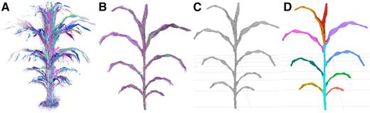
Processing of image data to segmented meshes. A, Point clouds are sampled from multiple perspectives around the plant. B, The point clouds are registered to the same frame and combined. C, The combined cloud is meshed to generate a set of polygons approximating the surface of the plant. D, The mesh is segmented into a shoot cylinder, leaves, and an inflorescence (if one exists; Supplemental Fig. S2), and phenotypes are measured automatically.
Most of the processing steps use generally applicable procedures available in open-source libraries and software, including registration, cleaning, and meshing of the point clouds (Cignoni et al., 2008; Rusu and Cousins, 2011; Buch et al., 2013; Kazhdan and Hoppe, 2013). General solutions for the segmentation of features like leaves and stems from plants, however, remain less developed, especially for 3D plant representations (Paproki et al., 2012; Paulus et al., 2013; Xia et al., 2015). Because of this, we developed a segmentation procedure for our particular application to partition the plant mesh into component parts. The final result of the semiautomated processing pipeline was a plant mesh segmented into a shoot cylinder, an inflorescence (when present; Supplemental Fig. S2), and individual leaves, with each individual leaf assigned a relative order of emergence (Fig. 1).
A total of 297 plants representing triplicate plantings of 99 plants (97 RILs and the two parental lines) from the BTx623 × IS3620C sorghum mapping population were grown in a greenhouse environment (Burow et al., 2011). Because image-based phenotyping is nondestructive, the same plant can be sampled at multiple time points to enable change over time to be monitored. All 297 plants were imaged at four time points over a 17-d interval starting 27 d after planting (DAP). The four time points, consisting of more than 14,000 depth images and representing nearly 1,200 samples, were processed to segmented meshes. As such, an individual plant was represented by a time course of four segmented meshes, and a RIL was represented by three biological replicates (Fig. 2). A series of measurements from each mesh was then automatically acquired (Table I).
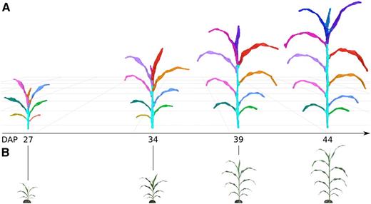
Plant growth over time. A, Segmented meshes for replicate 3 of RIL 175 are depicted at four different DAP time points. Leaf colors represent individual segmented leaves and have been assigned manually to enable tracking of the same leaf between meshes; Supplemental Figure S3 depicts how color is assigned automatically by the platform. The shoot cylinder is colored cyan. Meshes are depicted at the same relative scale. B, RGB data (not to scale) that correspond to the imaged plants and were coacquired with depth images; Supplemental Figure S3 depicts original RGB images.
Summary of the subset of traits automatically measured from the plant mesh used for the reported QTL analyses
Additional descriptions of the methods used to obtain the measurements are found in Supplemental File S1.
| Trait Type | Measurement | Description of Measured Trait |
|---|---|---|
| Composite | Shoot height | Vertical distance from the lowest shoot point to the highest shoot point, including leaves and inflorescence |
| Shoot surface area | Surface area of the entire shoot | |
| Shoot center of mass | Vertical distance from the lowest shoot point to the shoot’s center of mass | |
| Shoot compactness | Surface area of the smallest convex polyhedron that contains the entire shoot (i.e. convex hull surface area) | |
| Organ level | Shoot cylinder height | Vertical distance from the lowest shoot cylinder point to the highest shoot cylinder point |
| Leaf length | Length of a leaf | |
| Leaf surface area | Surface area of a leaf | |
| Leaf width | Width of a leaf | |
| Leaf angle | Angle at which a leaf emerges from the shoot cylinder |
To compare the measurements obtained from the image acquisition and processing platform with standard physical measurements of plant morphometric traits, 15 plants (with 140 leaves) from the experiment were imaged, and then leaf and stem measurements were obtained from harvested plants 62 d after planting. Shoot height, shoot cylinder height, leaf angle, leaf width, leaf length, and leaf area were compared. Leaf width and leaf length were measured using both a measuring tape and an LI-3100C Area Meter (LI-COR), and leaf area was measured using only the LI-COR instrument. Comparisons between the measurements indicated that the image-based measurements performed at least as well as the LI-COR leaf-scanning instrument for leaf width and leaf length relative to hand measurements with a measuring tape (Fig. 3). The RMSD between manual measurements and image-based measurements for leaf length and leaf width were 7.94 and 1.84 cm, respectively; this indicated marginally better performance than the RMSDs between manual measurements and the LI-COR instrument for leaf length and leaf width, which were 9.41 and 1.94 cm, respectively. Leaf area measurements made with the depth imaging platform and with the LI-COR instrument were well correlated (ρ of 0.92), although the image-based platform reported, on average, larger values of leaf area than the LI-COR instrument, with a mean difference of 52.45 cm2. Leaf angle was measured with an RMSD of 9° and a ρ of 0.95 relative to hand measurements, and shoot cylinder height was measured with an RMSD of 7 cm and a ρ of 0.99. Measurements of shoot height showed the lowest correlation (ρ = 0.63 and RMSD = 11 cm) due to three outlier points; these outlier points likely represent errors in manual measurement due to the inherent difficulty in identifying the true maximum height point of the shoot in an unbiased way during manual measurement. We also note two leaf measurement outliers in both leaf length and leaf area that occurred because the image-based platform failed to fully reconstruct two of the leaves that were in the same vertical plane as the sensor. Ultimately, image-based measurements were well correlated with manual measurements, and the coefficient of variation of the RMSD for the measurements ranged from 0.07 to 0.3 (within the same range as measurements made using standard instrumentation). As such, measurements made with the phenotyping platform have utility for applications such as QTL mapping.
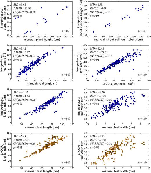
Comparison of image-based measurements with measurements made using standard methods. Axes represent measurements made via one of three methods: image-based measurements made from plant meshes, manual measurements made with a measuring tape or protractor, and measurements with a LI-COR LI-3100C Area Meter. Plots with an axis representing image-based measurements are colored blue, and plots without an axis representing image-based measurements are colored orange. Leaf area measurements made with the platform include abaxial and adaxial leaf surfaces, so the image-based area measurements were divided by two for comparison with LI-COR measurements of area. MD, Mean difference between measurements; RMSD, root-mean-square difference; CV(RMSD), coefficient of variation of the RMSD given the range of data on the bottom axis; ρ, Pearson product-moment correlation coefficient; n, number of samples from which the differences and coefficients were calculated.
Genetic Bases of Imaged Traits
To determine if the platform could be used to identify genetic loci regulating shoot architecture, measurements obtained from the plant meshes were associated with genetic data from the RIL population. Genotypes for members of the BTx623 × IS3620C RIL population were obtained previously and available to construct a genetic map for mapping QTLs for the image-based phenotypes across multiple developmental time points (Morishige et al., 2013; Truong et al., 2014; McCormick et al., 2015). Measurements obtained from plant meshes were grouped into two categories: organ-level measurements and composite measurements. Organ-level measurements are segmentation dependent and measure organ-level plant architecture, such as leaf length and shoot cylinder height; composite measurements are segmentation independent and measure overall shoot architecture, such as shoot height and shoot compactness (Table I; Supplemental Figs. S4 and S5).
QTL mapping of organ-level traits identified seven unique genomic intervals with significant contributions to phenotypic variability (Fig. 4; Supplemental Fig. S6; Supplemental Table S1). A genome-wide scan under a single-QTL model was used to examine the following phenotypes across the four time points: the average value of leaves 3, 4, and 5 for leaf length, width, surface area, and inclination angle as well as shoot cylinder height. Significant QTLs identified from a genome-wide scan under a single-QTL model were used as an initial model for stepwise model traversal to identify the most likely penalized multiple-QTL model (Manichaikul et al., 2009); the overlapping LOD-2 intervals of these multiple-QTL models define unique intervals on chromosomes 3, 4, 6, 7, and 10 (Supplemental Table S1).
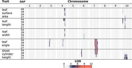
Log of the odds (LOD) profiles for organ-level traits. For each phenotype, LOD profiles are based on chromosome-wide scans of chromosomes with QTLs based on the most likely multiple-QTL models found by model selection (Supplemental Fig. S6). Each row represents a different trait, and within each trait are four nested rows that each represents a different time point (DAP). Each group of columns represents a chromosome, and each column represents a marker at its genetic position. Cells are colored by marker LOD for the phenotype at the particular time point.
A major source of variation in shoot architecture in the BTx623 × IS3620C RIL population is Dwarf3 (Dw3), a sorghum dwarfing gene on chromosome 7 at 59.8 Mb. The parents of the imaged RIL population, BTx623 and IS3620C, are fixed for nonfunctional and functional forms, respectively, of the Dw3 gene, which encodes an auxin efflux protein that has pleiotropic effects on stem elongation and additional architecture traits like leaf angle (Multani et al., 2003; Truong et al., 2015). A significant association between Dw3 and shoot cylinder height is not observed until the second time point (34 DAP), while different alleles of Dw3 introduce significant variability in leaf angle by the earliest time point (27 DAP). This is likely because Dw3 impacts height by impacting stem elongation and the stem has not yet begun to elongate substantially by the earliest time point; as such, the nonfunctional dw3 allele caused smaller leaf angles prior to any significant effect on stem elongation (Multani et al., 2003; Truong et al., 2015). Similar to Dw3, the effects of Dw2, a sorghum dwarfing gene on chromosome 6 near 42 Mb (but not yet cloned), are significantly associated with shoot cylinder height after the first time point (34, 39, and 44 DAP); unlike Dw3, Dw2 is not significantly associated with any other pleiotropic effects on leaf morphology. However, an interval distinct from Dw2 is observed on chromosome 6 near 51 Mb for leaf width.
A large interval on chromosome 10 was significantly associated with variability in leaf length and surface area as well as shoot cylinder height. While the LOD-2 intervals for these traits overlapped when comparing all phenotype-by-time point combinations, the LOD-2 interval for leaf surface area at 39 DAP was distinct from any shoot cylinder height intervals. Additionally, the significant association of the interval with shoot cylinder height is lost after 34 DAP, while the association is maintained with leaf traits throughout the time course, suggesting that multiple QTLs that regulate shoot architecture are present on chromosome 10 (Supplemental Table S1).
An interval on chromosome 4 was associated with multiple leaf traits, including length, width, and surface area, measured as the average value of leaves 3, 4, and 5 when counting green leaves starting from the bottom of the plant at the time of acquisition. Further analysis showed that plants with BTx623 alleles of an insertion/deletion (indel) marker at the leaf length maximum log of the odds (MLOD) coordinate (chromosome 4; 62.45 Mb) had a leaf length of 50.1 cm when averaged across the four time points. This was 5.6 cm longer than plants with IS3620C alleles, which had a leaf length of 44.5 cm when averaged across the four time points. Additionally, the platform captured changes in leaf length over time; plants with BTx623 alleles increased from an average length of 44.2 cm to an average length of 54.8 cm over the 17 d, whereas plants with IS3620C alleles had leaves that increased from an average length of 40.1 cm to an average length of 47.5 cm (Fig. 5).
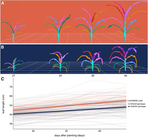
Organ-level measurement of average leaf length over time. A and B, Meshes displaying development over time for a plant bearing BTx623 alleles (A; RIL 257) and a plant bearing IS3620C alleles (B; RIL 306) of an indel marker on chromosome 4 that had the MLOD for leaf length. C, Change in average leaf length over time. Each thin line in the plot represents the average leaf length of a RIL (n = 3) colored by its genotype. Leaf length was calculated as the average of the third, fourth, and fifth leaves counting from the bottom, corresponding to the light green, dark green, and blue leaves in A and B. The two thick lines represent a linear fit for each genotype and 95% confidence intervals.
Because segmentation-dependent traits represent organ-level traits that are often manually measured, QTLs identified via the image-based platform for organ-level traits were compared with QTLs identified previously for similar traits in the BTx623 × IS3620C population and previous reports on the sorghum dwarfing loci Dw2 and Dw3 (Hart et al., 2001; Feltus et al., 2006; Brown et al., 2008; Mace and Jordan, 2011; Morris et al., 2013; Higgins et al., 2014). Most organ-level QTL intervals found in this study overlap with comparable or related traits from previous field studies (Table II). Of note, some of the intervals, like chromosome 6 near 51 Mb and chromosome 4 near 62 Mb, may have multiple genes that each affect different traits or genes with pleiotropic effects, since these intervals were associated with diverse leaf morphology traits across the studies. Additionally, the genes involved could be environmentally responsive, since related but different traits were associated for the intervals when comparing the greenhouse-based and field-based studies (e.g. leaf length in this study versus leaf pitch, but not leaf length, in the previous study, where leaf pitch measures the length of the leaf from the leaf base to the apex of the naturally curved leaf). Overall, there was extensive overlap between the QTL intervals identified in previous work and those identified using the imaging platform, suggesting that these genomic loci exert phenotypic effects across multiple studies and environments.
Comparison of QTL intervals identified using image-based phenotyping with previously reported QTL intervals in the literature
Most QTL intervals identified with the platform overlapped with QTLs or causal genes reported previously for related phenotypes (Hart et al., 2001; Feltus et al., 2006; Mace and Jordan, 2011; Morris et al., 2013; Higgins et al., 2014). Dw3 was cloned previously (Multani et al., 2003). For image-based QTL intervals, the LOD-2 interval and peak coordinate for the phenotype with the maximum MLOD are reported, and the phenotype name is indicated by an asterisk; maximum MLOD coordinates are not applicable to intervals from the literature, indicated by a dash. Supplemental Table S1 contains all identified organ-level QTLs. Leaf pitch and leaf curve are both measures of Euclidean distance from the leaf base to the apex of the curved leaf blade and from the leaf base to the leaf tip, respectively (Feltus et al., 2006).
| Chromosome | Origin | Interval Begin | Max MLOD Coordinate | Interval End | Related Traits with Overlapping Intervals | Prior Locus Names |
|---|---|---|---|---|---|---|
| Mb | ||||||
| 4 | Image based | 57.48 | 62.45 | 63.40 | Leaf length*, leaf surface area, leaf width | QLcv.txs-D2, QLpt.txs-D |
| Literature | 61.86 | – | 65.07 | Leaf curve, leaf pitch | ||
| 6 | Image based | 40.10 | 42.77 | 44.83 | Shoot cylinder height* | Dw2 |
| Literature | 39.72 | – | 42.64 | Preflag leaf height | ||
| Image based | 48.45 | 50.97 | 55.08 | Leaf width* | QLcv.txs-I | |
| Literature | 53.73 | – | 56.52 | Leaf curve | ||
| 7 | Image based | 59.51 | 59.65 | 59.99 | Leaf angle*, shoot cylinder height | Dw3 |
| Literature | 59.821905 | – | 59.829910 | Leaf angle, culm height, culm uniformity | ||
| 10 | Image based | 1.23 | 2.00 | 8.21 | Leaf length*, leaf surface area | QLcv.txs-G, QLpt.txs-G, QLln.txs-G, QHtu.txs.G, QHGT_meta1.10 |
| 5.27 | 7.46 | 52.24 | Shoot cylinder height* | |||
| Literature | 1.11 | – | 5.76 | Leaf curve, leaf pitch | ||
| 6.40 | – | 13.05 | Leaf length, culm height, culm uniformity |
In addition to capturing components of plant architecture like leaf morphology, the image-based measurements also capture overall architecture traits that integrate component traits. These composite measurements are difficult or impossible to measure by hand and integrate how component traits interact to influence overall plant architecture and, ultimately, how a plant canopy intercepts solar radiation. One specific example of such a measurement is shoot compactness, measured as the surface area of the convex hull of a plant mesh. Shoot compactness is influenced by factors like leaf angle and the height and planarity of a plant (Supplemental Fig. S5). Accordingly, a strong association between Dw3 and shoot compactness is present at all time points due to the consistent effects of Dw3 on leaf angle and later effects of Dw3 on stem growth (Fig. 6). As such, composite traits represent measures of overall plant architecture and integrate the interrelationships between component phenotypes. Additional composite traits examined were shoot surface area, shoot center of mass, and shoot height, as described in Table I.
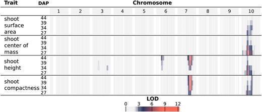
LOD profiles for composite traits. For each phenotype, LOD profiles are based on chromosome-wide scans of chromosomes with QTLs based on the most likely multiple-QTL models found by model selection (Supplemental Fig. S7). Each row represents a different trait, and within each trait are four nested rows that each represents a different time point (DAP). Each group of columns represents a chromosome, and each column represents a marker at its genetic position. Cells are colored by marker LOD for the phenotype at the particular time point.
QTL mapping of the selected composite traits identified four genomic intervals with significant contributions to phenotypic variability (Fig. 6; Supplemental Fig. S7; Supplemental Table S2). Since composite traits are expected to be driven by phenotypic variation in their component traits (and thus correlated), the composite trait QTLs are discussed in the context of organ-level QTLs with shared intervals. All of the composite traits were significantly associated with a large interval on chromosome 10 at early stages of development (27 and 35 DAP). Consistent with the observation of nonoverlapping QTL intervals for organ-level traits of leaf morphology and shoot cylinder height on chromosome 10, at least two QTLs are likely present in the interval; canopy compactness is a trait influenced by both leaf morphology and shoot height, and distinct LOD peaks were observed, one at 6 Mb and one at 52 Mb (Supplemental Table S2).
Interestingly, one interval unique to the composite trait measurements was identified on chromosome 3 near 66 Mb for shoot height, indicating that there are additional component traits driving variability in overall architecture that remain to be resolved and explained by organ-level traits. Alternatively, the impact of the QTLs on individual organ-level traits is relatively small, and only the combined effects across multiple individual traits provide sufficient power for detection. As such, these composite traits represent a useful approach for detecting novel genetic loci.
Due to the effect of Dw3 on shoot cylinder height and leaf angle, a strong association is present for shoot height and shoot compactness at the Dw3 locus; likewise, Dw2 is associated with shoot height. To further quantify the influence of Dw3, the shoot heights of individuals bearing different alleles of an indel marker near Dw3 were compared. Plants that have the dominant, functional Dw3 allele increase in height from, on average, 60.2 to 112.6 cm over the 17-d imaging interval, and plants with nonfunctional dw3 alleles increase in average height from 56.8 to 93.2 cm (Fig. 7). Fitting a linear model to the data, Dw3 plants grew vertically at a rate of 3.1 cm d−1, whereas dw3 plants grew at a rate of 2.2 cm d−1 between 27 and 44 DAP. Nondestructive, image-based phenotyping combined with high-throughput genotyping has great potential for parameterizing plant functional-structural modeling and performance prediction with genotype-specific rates of growth.
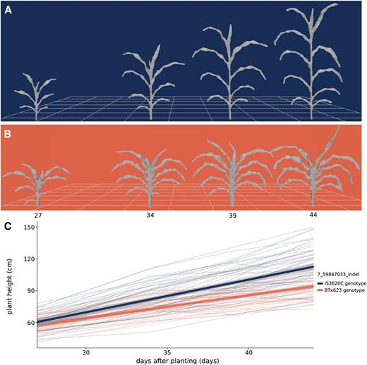
Composite measurement of shoot height over time. A and B, Meshes displaying development over time for a plant bearing IS3620C alleles (A; RIL 175) and BTx623 alleles (B; RIL 19) of an indel marker closely linked with the Dw3 gene, an auxin transporter that regulates plant height. C, Change in plant height over time. Each thin line in the plot represents the average height of a RIL (n = 3) colored by its genotype at the Dw3 locus. Shoot height was measured as the vertical distance from the lowest shoot point to the highest shoot point, including leaves and inflorescence (Table I). The two thick lines represent a linear fit for each genotype at Dw3 and 95% confidence intervals.
DISCUSSION
A time-of-flight depth camera was used to image sorghum plants from a RIL population, and we developed an image processing pipeline to reconstruct 3D sorghum plants and make automated measurements from the reconstructions. Measurements made in this manner are sufficiently rapid and accurate to enable the identification of multiple genetic loci regulating shoot architecture. As such, we demonstrate that depth imaging represents a useful approach for high-throughput phenotyping of crop plant architecture for the genetic dissection of complex traits.
While the platform successfully identified QTLs regulating sorghum architecture (Figs. 4 and 6), a number of improvements will be necessary prior to its applicability in even larger scale studies. First, the acquisition process will need to be improved. Registration artifacts were a recurring problem, introduced by nonrigid transformations of plant leaves caused by leaf shaking on the turntable, the registration methods used, and sensor noise in acquisition. Multiple potential solutions for these are available, including the use of a registration algorithm capable of handling nonrigid transformations (Zheng et al., 2010; Bucksch and Khoshelham, 2013; Brophy et al., 2015), the use of multiple sensors, the use of real-time mesh construction procedures like Kinect Fusion to average sensor data and rapidly reconstruct the plant (Izadi et al., 2011), or the use of a model-based approach to fit a geometric plant model to the acquired points (Quan et al., 2006; Ma et al., 2008). Second, the segmentation procedure will need to be improved to better distinguish leaves that are in contact with one another, to better automatically identify the shoot cylinder of the plant, and to potentially make it applicable to other grass or plant species. Progress in data-driven approaches that automatically cluster points into stem and leaf organs using feature histograms indicate that segmenting point clouds directly represents a viable option, at least for high-resolution laser scans (Paulus et al., 2013; Wahabzada et al., 2015). Segmenting the point cloud directly may provide the most general solution for both controlled-environment and field applications, where reconstruction prior to segmentation is difficult due to occlusion. Approaches that can accurately segment the point cloud directly also could enable automated fitting of generalized plant or organ models to the segmented cloud, potentially yielding methods that can automatically reconstruct and measure complex plant scenes.
A major benefit of image-based phenotyping is its nondestructive nature because insight into the temporal onset of genetic regulation is valuable in dissecting its mechanistic basis. Markers tightly linked with Dw3, a gene encoding an auxin transporter, are associated with leaf inclination angle and shoot compactness prior to their association with shoot height and shoot cylinder height, suggesting that changes in auxin transport caused by different Dw3 alleles introduce variability in leaf development and overall shoot compactness prior to large effects on stem elongation (Figs. 4, 6, and 7). Additionally, variation in the shoot cylinder height at the earliest time point is most associated with an interval on chromosome 10 (Fig. 4). This QTL is the primary driver of variability in shoot height and shoot cylinder height until the variability in stem growth introduced by alleles of Dw2 and Dw3 increases, and it may be related to the timing of a developmental transition (Figs. 4 and 6). It is likely that multiple QTLs are present on chromosome 10, given that distinct LOD peaks at 2, 7, and 52 Mb were observed; additional experimentation will be necessary to resolve the contributions and temporal prevalence of specific QTLs in the interval.
Many of the QTLs identified via image-based phenotyping overlapped with QTLs for comparable traits discovered in prior field experiments (Table II). These shared QTLs represent good candidates for continued investigation, as they display robust phenotypic effects across multiple experiments and conditions. Notably, despite sharing overlapping intervals, the associated traits sometimes differed. For example, this study identified significant associations between leaf length, width, and surface area with an interval on chromosome 4; a similar interval was identified in previous work for leaf curve and leaf pitch, but it was not significantly associated with leaf length in the previous study (Table II). While all of these traits are aspects of leaf morphology and share relationships, additional experimentation will be necessary to determine whether these represent one QTL with pleiotropic effects (as observed with Dw3), one QTL with different environmental responses, different QTLs with overlapping intervals, or some combination of these possibilities.
CONCLUSION
Depth imaging and subsequent processing enabled the rapid acquisition of multiple shoot architecture phenotypes from a sorghum RIL population, and genetic loci contributing to variation in shoot architecture were identified. Depth cameras represent a practical tool to rapidly measure plant morphology, and their application to plant phenotyping alongside other imaging modalities will be useful for both controlled-environment and field phenotyping scenarios. Integrated platforms that merge image-based phenotyping approaches, genetics, and performance modeling will enable rapid improvements in understanding plant biology and will promote the selection and engineering of plants for superior performance in target applications.
MATERIALS AND METHODS
Plants, Greenhouse Conditions, Manual Measurements, and Image Acquisition
A total of 98 RILs from the sorghum (Sorghum bicolor) BTx623 × IS3620C recombinant inbred mapping population and the two parents (Burow et al., 2011) were planted in triplicate with five seeds per pot in C600 pots of Sunshine MVP soil (BWI) in a College Station, Texas, greenhouse on July 7, 2015. Plants were thinned to one plant per pot after germination. Plants were fertilized with Osmocote Classic (13-13-13; Everris International) and watered on demand. Tillers and senesced leaves were removed regularly. Each of the three replicates of the 100 lines was grown on a separate greenhouse table, and differences in shoot morphology were visibly apparent in the population throughout development (Supplemental Figs. S8 and S9). Seeds for one of the RILs failed to germinate (RIL 3), leaving three replicates of 99 lines for which images were acquired. Plants were imaged at 27, 34, 39, and 44 DAP. Fifteen of the plants were imaged at 62 DAP, harvested, and manually measured to compare the performance of the platform relative to standard measurement techniques. Manual measurements of leaf angle were made with a protractor, and shoot height, shoot cylinder height, leaf length, and leaf width were measured using a measuring tape. Additionally, leaf length, leaf width, and leaf area were measured using an LI-3100C Area Meter (LI-COR).
Image acquisition was performed using a Microsoft Kinect for Windows version 2 sensor and the Kinect for Windows SDK (version 2.0). Twelve RGB and 12 depth image frames were acquired at approximately 3-s intervals, and the images were saved to disk on a laptop while the Kinect for Windows version 2 sensor was positioned on a tripod in front of an Arqspin 12-inch motorized turntable that rotated the imaged plant (Supplemental Fig. S1). Plants were transported manually to and from the greenhouse to the nearby imaging station. Images were transferred from the laptop to a work station for subsequent processing.
Processing Images to Acquire Plant Measurements
Procedures for processing images to acquire plant measurements and alternative methods that were explored are explained in Supplemental File S1. Here, brief descriptions of procedures used for the reported analysis are outlined. For each plant, the point cloud contained in each depth image was automatically cleaned and registered to generate a single 3D point cloud using available open-source libraries and algorithms, including OpenCV (http://opencv.org; accessed February 2016) and PCL (Fischler and Bolles, 1981; Besl and McKay, 1992; Rabbani et al., 2006; Rusu et al., 2008; Rusu and Cousins, 2011; Buch et al., 2013). This point cloud was inspected manually, acquisition and/or registration errors were corrected manually using MeshLab (Cignoni et al., 2008), and the cleaned point cloud was meshed to generate a set of polygons representing the surface of the plant using available open-source software (Bernardini et al., 1999; Corsini et al., 2012; Kazhdan and Hoppe, 2013). The plant mesh was then segmented into a shoot cylinder (composed of the stem and leaf sheaths), individual leaves, and an inflorescence (when present; Supplemental Fig. S2). The shoot cylinder and inflorescence were labeled manually. Following this, individual leaves were segmented using an automated procedure we developed that uses supervoxel adjacency and geodesic paths across the adjacency graph to identify leaf tips and grow leaf regions (Dijkstra, 1959; Surazhsky et al., 2005; Papon et al., 2013).
Multiple measurements were automatically obtained from each mesh, both at the level of the whole plant (i.e. segmentation-independent, composite traits) and at the organ level (i.e. segmentation-dependent, organ-level traits). The traits measured are described in Table I. Descriptions of how these traits were measured from the plant mesh are provided in Supplemental File S1, and graphical depictions of selected measurements are shown in Supplemental Figures S4 and S5. Additional implementation details can be found with the code base (see “Code and Data Availability” below).
QTL Mapping and Comparison with Prior QTL Studies from the Literature
Genotypes for the BTx623 × IS3620C RIL population were generated previously using Digital Genotyping, a restriction enzyme-based, reduced-representation sequencing assay (Morishige et al., 2013). Genotypes were called using the naive pipeline of the RIG workflow with the GATK, and the genetic map was constructed as described previously with marker orderings relative to the version 3 assembly of the sorghum reference genome, Sbi3 (Department of Energy-Joint Genome Institute [http://phytozome.jgi.doe.gov]; accessed February 2016); this resulted in a genetic map with 10,787 markers (McKenna et al., 2010; Goodstein et al., 2012; Truong et al., 2014; McCormick et al., 2015). Both single- and multiple-QTL mapping were performed with R/qtl (Broman et al., 2003). For single-QTL mapping (i.e. testing a single-QTL model), the complete marker set of 10,787 markers was used. Measurements of a trait for each of the three replicates of a RIL were averaged; average trait values were normalized using empirical normal quantile transformation prior to QTL mapping, so that the same permutation threshold would apply to all phenotype-by-time point combinations (Peng et al., 2007). A genome-wide scan under a single-QTL model for each phenotype-by-time point combination was performed (Supplemental Figs. S6 and S7). If any of the reported phenotype-by-time point combinations had a marker with a LOD greater than 3.28 (the 95% threshold obtained from 25,000 permutations), its LOD-2 interval (the coordinates of the flanking markers where the LOD had dropped by 2 units below the peak value) was retained. The positions (centimorgans) with the largest LOD within each LOD-2 interval for each phenotype-by-time point combination were retained to initialize multiple-QTL mapping.
For multiple-QTL mapping, a subset of 1,209 markers was obtained by enforcing a minimum marker distance of 0.8 centimorgans; significant peak-LOD markers from single-QTL mapping intervals were added back to the set if they were dropped, resulting in 1,224 markers used for multiple-QTL mapping. The genetic coordinates of the markers with the largest LOD for each LOD-2 interval from single-QTL mapping of each phenotype-by-time point combination were used to seed model selection for multiple-QTL mapping as implemented in R/qtl (Manichaikul et al., 2009). Main effect, heavy chain, and light chain penalties (3.2, 4.38, and 1.94, respectively) for model selection were obtained as 95% thresholds from 25,000 permutations of the appropriate statistics. The multiple-QTL models with the largest penalized LOD for each phenotype-by-time point combination are reported (Table II; Supplemental Tables S1 and S2; Supplemental Figs. S6 and S7). For a given phenotype, the maximum LOD across all time points characterized the MLOD of the phenotype (Kwak et al., 2014). A longitudinal QTL model for each phenotype that contained QTLs at the MLOD coordinates was used to generate the chromosome-wide LOD profile scans (Figs. 4 and 6).
To compare QTLs found in this study with existing QTLs in the literature, the physical coordinates relative to the sorghum version 1 reference assembly, Sbi1, for QTLs in the BTx623 × IS3620C population were obtained; Mace and Jordan (2011) determined these physical coordinates using a consensus map and QTLs identified by Hart et al. (2001) and Feltus et al. (2006). The coordinates of Dw2 and Dw3 were obtained from Morris et al. (2013) and Multani et al. (2003). The corresponding locations of the markers in Sbi3 were obtained using Biopieces for sequence extraction and BLAST via a local instance of Sequenceserver (Altschul et al., 1997; Paterson et al., 2009; Priyam et al., 2015; www.biopieces.org). Physical locations relative to Sbi3 were used as the QTL intervals for comparison with this study.
Code and Data Availability
The C++, Bash, and Python code written for image acquisition and processing, the R code written for QTL mapping, the genotype and phenotype data, and the full multiple-QTL models for each phenotype-by-time point combination can be found on GitHub at https://github.com/MulletLab/SorghumReconstructionAndPhenotyping. For each imaged plant, its depth images, a single RGB image, and the segmented mesh can be found at the Dryad Digital Repository (http://dx.doi.org/10.5061/dryad.9vs26).
Supplemental Data
The following supplemental materials are available.
Supplemental Figure S1. Imaging platform.
Supplemental Figure S2. Plants with inflorescences.
Supplemental Figure S3. Plant growth over time.
Supplemental Figure S4. Visual depiction of selected measurements.
Supplemental Figure S5. Composite traits integrate multiple architecture traits.
Supplemental Figure S6. QTL mapping steps for organ-level traits leading to the final LOD profiles shown in Figure 4.
Supplemental Figure S7. QTL mapping steps of composite traits leading to the final LOD profiles shown in Figure 6.
Supplemental Figure S8. BTx623 × IS3620C RIL population in the greenhouse.
Supplemental Figure S9. Plants from the BTx623 × IS3620C RIL population display variation in shoot morphology.
Supplemental Table S1. QTL intervals by phenotype for organ-level traits.
Supplemental Table S2. QTL intervals by phenotype for composite traits.
Supplemental File S1. Image processing methods, potential alternatives, and future development.
ACKNOWLEDGMENTS
We thank Sergio Hernandez for assistance during image acquisition; Marcin Kalicinski for RapidXML, which is used to parse configuration files during mesh processing (http://rapidxml.sourceforge.net/; accessed February 2016); the Blender Foundation for the 3D modeling and rendering package, Blender, which was used to stage meshes for the figures (https://www.blender.org/; accessed February 2016); the Texas A&M Institute for Genome Sciences and Society for maintaining the TIGSS HPC Cluster, which was used to calculate main effect, heavy chain, and light chain penalties for multiple-QTL mapping; and the anonymous reviewers for providing constructive feedback during the review process.
Glossary
- 3D
three-dimensional
- RIL
recombinant inbred line
- QTL
quantitative trait locus
- RGB
red-green-blue
- DAP
days after planting
- RMSD
root-mean-square difference
- LOD
log of the odds
- indel
insertion/deletion
- MLOD
maximum log of the odds
LITERATURE CITED
Author notes
This work was supported by the Department of Energy Great Lakes Bioenergy Research Center (grant no. BER DE–FC02–07ER64494) and the U.S. Department of Energy (grant no. DE–AR0000596).
Address correspondence to [email protected].
The author responsible for distribution of materials integral to the findings presented in this article in accordance with the policy described in the Instructions for Authors (www.plantphysiol.org) is: John E. Mullet ([email protected]).
R.F.M. developed the image acquisition and analysis software; R.F.M. and S.K.T. managed the plants, acquired image data, and analyzed the data; R.F.M., S.K.T., and J.E.M. designed the experiments and wrote the article.
Articles can be viewed without a subscription.
