


Abstract
The effect of the surrounding environment of supernova remnant shocks on nonthermal X-rays from accelerated electrons, with or without interacting dense material, is an open issue. We conduct spatially resolved X-ray spectroscopy of the shock–cloud interacting region of RCW 86 with XMM–Newton. It is found that bright soft X-ray filaments surround the dense cloud, observed with 12CO and H i emission lines. These filaments are brighter in thermal X-ray emission, and fainter and possibly softer in synchrotron X-rays, compared to those without interaction. Our results show that the shock decelerates due to the interaction with clouds, which results in an enhancement of thermal X-ray emission. This could possibly also explain the softer X-ray synchrotron component, because it implies that those shocks that move through a low-density environment, and therefore decelerate much less, can be more efficient accelerators. This is similar to SN 1006 and Tycho, and is in contrast to RX J1713.7−3946. This difference among remnants may be due to the clumpiness of dense material interacting with the shock, which should be examined in future observations.
1 Introduction
Shocks of supernova remnants (SNRs) are the most plausible site of Galactic cosmic ray acceleration. Together with X-ray observations, it is known that the magnetic field on the shocks is amplified and turbulent, which gives thin and bright synchrotron X-ray filaments or knots on the shock (e.g., Vink & Laming 2003; Bamba et al. 2003, 2005; Bell 2004; Uchiyama et al. 2007). One of the most important remaining problems is what kind of environment gives such a magnetic field amplification—when the maximum energy of accelerated electrons is limited by synchrotron cooling, it is proportional to the square of the shock velocity (e.g., Aharonian & Atoyan 1999; Yamazaki et al. 2006; Zirakashvili & Aharonian 2007), implying that low-density environments make the maximum energy larger since the shock remains fast with a low deceleration. In fact, many synchrotron X-ray-dominated SNRs emit no or only faint thermal X-ray emission (Koyama et al. 1997; Slane et al. 2001; Bamba et al. 2001, 2012; Yamaguchi et al. 2004). Lopez et al. (2015) used spatially resolved spectroscopy to study Tycho with NuSTAR, and showed that the high-shock-speed regions have high-energy synchrotron X-ray cut-offs. On the other hand, Inoue et al. (2009, 2012) suggested that the shock–cloud interaction amplifies the turbulent magnetic field. Such clumpy clouds also affect the GeV–TeV spectra from supernova remnants and X-ray variability (Celli et al. 2019). Sano et al. (2013) discovered some molecular cloud clumps in RX J1713.7−3946 surrounded by synchrotron X-ray filaments, and Sano et al. (2015) showed that high interstellar gas density regions tend to have harder X-ray spectra in this remnant. These results confirm the scenario that a clumpy medium enhances turbulence and hence facilitates X-ray synchrotron emission. We need more samples to investigate what happens in the shock–cloud interacting regions in supernova remnants.
RCW 86 is one of the SNRs emitting synchrotron X-rays (Bamba et al. 2000; Borkowski et al. 2001b), GeV gamma-rays (Lemoine-Goumard et al. 2012; Yuan et al. 2014), and very high-energy gamma-rays (H.E.S.S. Collaboration et al. 2018). An interesting characteristic of this SNR is that it emits not only synchrotron X-rays but also thermal X-rays, which makes this target unique among synchrotron X-ray-dominated SNRs. The ratio of thermal and synchrotron X-rays in RCW 86 is different from position to position (Broersen et al. 2014; Tsubone et al. 2017), especially on the eastern rim (Vink et al. 2006), which could be due to the location dependence of the shock wave velocity. The shock velocity measured by proper motion also changes rapidly, especially on the eastern side (Yamaguchi et al. 2016). This could be connected to the fact that the south-eastern part interacts with 12CO and/or H i clouds (Sano et al. 2017, 2019). These facts make this SNR ideal for the study of the effect of shock–cloud interaction on particle acceleration.
In this paper, we study the spatially resolved spectroscopy of the RCW 86 shock–cloud interacting region, together with X-ray and CO map comparisons, in order to understand how the interaction affects particle acceleration. Section 2 describes the data set as well as the data reduction. The imaging and spectral analysis results are described in section 3. Finally, we discuss our results in section 4. Throughout this paper, we adopt 2.3 kpc as the distance to our target (Sollerman et al. 2003; Helder et al. 2013).
2 Observations and data reduction
The south-eastern region of RCW 86 was observed with XMM–Newton (Jansen et al. 2001) on 2014 January 27. The data reduction and analysis were done with SAS version 20.0.0 (Gabriel et al. 2004). We selected only the data taken by the MOS cameras (Turner et al. 2001) since the MOS camera has a better energy resolution and a lower background level compared with the pn camera. We used the cleaned data with the standard XMM–Newton method following the SAS guide, and the resultant exposure time is 101 ks. For the spectral analysis, we used XSPEC 12.12.1 in headas 6.30.1.
3 Results
3.1 Images
Figure 1 shows MOS2 0.5–2.0 keV (red) and 2.0–8.0 keV (blue) images of the south-eastern region of RCW 86. We did not use MOS1 for the image analysis since several chips are not in operation. The 12CO(J = 2–1) map is also overlaid with white contours. One can see that several X-ray filaments beautifully surround the molecular clouds within a scale of ∼1″ or ∼0.7 pc at a 2.3 kpc distance, as if these filaments are aware of the contour levels, a result already reported in the original paper by Sano et al. (2017).
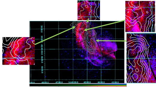
MOS2 0.5–2.0 keV (red) and 2.0–8.0 keV (blue) band images of the south-eastern region of RCW 86 on logarithmic scales. The images are binned with 64 × 64 pixels. The vignetting correction and non-X-ray-background subtraction are not performed. The color range is between 0.2–20 cnt per binned pixel for the 0.5–2.0 keV band, and 0.2–5 cnt per binned pixel for the 2.0–8.0 keV band. Coordinates are in J2000. White contours represent the 12CO(J = 2–1) distribution in the velocity range of −36 to −34 km s−1 taken by NANTEN2 (see figure 6 of Sano et al. 2017). The small panels are close-up views of the bright filaments.
This result is already claimed by Sano et al. (2017). The filaments surrounding the molecular clouds looks red, implying that their X-ray emission is softer than those from non-interacting regions.
One can see that there are soft X-ray filaments extending south-west beyond the molecular cloud. We thus examined whether there is dense material on these filaments in the Australia Telescope Compact Array (ATCA) H i map taken by Sano et al. (2017). Figure 2 shows the same MOS2 map with H i contours. It is found that there is an associated H i cloud in the velocity range between −35 and −30 km s−1, which is similar in range to the velocity of the 12CO clouds that are associated with the SNR. The filaments are on the edge of the H i cloud, which is the same situation as in the northern CO cloud cases.

3.2 Spectra
In order to examine the spectral difference among the filaments, we selected 13 regions for the spectral analysis, as shown in figure 3. The dashed areas indicate background regions. Since several regions are located outside of the MOS1 field of view due to the lack of a CCD chip, we used only the MOS2 camera data for such regions (src1, 3, 4, 5, and 6).
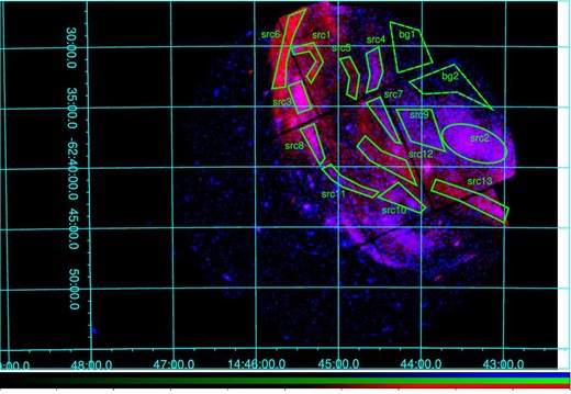
Same MOS2 images as in figure 1, with source and background (solid and dashed, shown in green) regions for the spectral analysis.
Figure 4 shows the background-subtracted spectrum for each region. One can see that some show softer spectra with emission lines, and others show harder spectra without lines. We thus fitted all spectra with a non-equilibrium thermal component (nei in XSPEC; Borkowski et al. 2001a) plus a power-law component to reproduce synchrotron X-rays. All the abundances are set to solar for the thermal emission. To represent the absorption model, we use the phabs model in XSPEC, which includes the cross-sections of Balucinska-Church and McCammon (1992) with solar abundances (Anders & Grevesse 1989). We used Cash statistics for the spectral fitting (Cash 1979). The data are all well reproduced by these models, as shown in table 1.
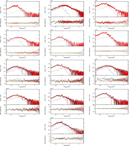
Spatially resolved spectra with best-fitting models. Black and red show the MOS1 and MOS2 data, respectively. The dotted lines represent the vnei and power-law components. The data are binned for better visibility, whereas the fitting is done without binning.
Best-fitting parameters for the spectral fitting.*
| Reg. | Area | NH | Γ | F2-10 keV† | kTe | net | Norm§ | F0.5-10 keV† | C-stat.|$/$|d.o.f. |
|---|---|---|---|---|---|---|---|---|---|
| (arcsec2) | (1021 cm−2) | (keV) | (1010 s cm−3) | ||||||
| src1 | 9349 | 4.1 | 3.11 | 0.17 | 0.43 | 1.4 | 30 | 23.5 | 1385.9|$/$|1533 |
| (3.7–5.1) | (2.45–3.85) | (0.09–0.28) | (0.25–0.57) | (1.0–4.2) | (17–135) | (17.3–36.3) | |||
| src2 | 44411 | 5.5 | 2.84 | 1.54 | —|| | —|| | 7.5 | 4.5 | 3339.3|$/$|3074 |
| (5.1–5.9) | (2.79–2.91) | (1.48–1.59) | (5.1–10.4) | (3.1–6.3) | |||||
| src3 | 10373 | 4.6 | 3.31 | 0.28 | 0.34 | 1.6 | 36 | 20.9 | 1736.3|$/$|1533 |
| (4.4–4.9) | (3.16–3.45) | (0.25–0.31) | (0.27–0.39) | (1.3–2.2) | (25–45) | (17.3–25.4) | |||
| src4 | 12114 | 5.6 | 3.25 | 0.41 | 0.24 | 6.2 | 16 | 4.8 | 1408.3|$/$|1533 |
| (3.6–6.8) | (2.85–3.49) | (0.35–0.47) | (0.18–4.78) | (0.4–28.6) | (0.9–72) | (0.7–12.1) | |||
| src5 | 9902 | 4.3 | 4.16 | 0.02 | 0.66 | 0.7 | 4.4 | 5.0 | 1269.9|$/$|1533 |
| (3.7–5.2) | (3.38–5.07) | (0.008–0.05) | (0.29–1.01) | (0.5–2.2) | (2.5–17.0) | (3.4–10.3) | |||
| src6 | 18934 | 4.5 | 4.49 | 0.14 | 0.34 | 2.0 | 171 | 104.0 | 1564.0|$/$|1533 |
| (4.1–4.7) | (4.10–4.85) | (0.06–0.18) | (0.32–0.45) | (1.3–2.3) | (94–190) | (76.9–108.9) | |||
| src7 | 11448 | 4.6 | 2.83 | 0.32 | 0.35 | 2.1 | 7.3 | 4.6 | 3042.2|$/$|3072 |
| (3.6–5.5) | (2.58–3.07) | (0.28–0.37) | (0.24–0.95) | (0.8–6.3) | (1.5–28) | (2.2–8.9) | |||
| src8 | 10301 | 4.8 | 2.86 | 0.38 | 0.24 | 2.5 | 57 | 18.8 | 3103.2|$/$|3072 |
| (4.1–5.9) | (2.69–3.09) | (0.33–0.43) | (0.18–0.35) | (1.1–10.6) | (19–240) | (10.8–38.2) | |||
| src9 | 28590 | 5.4 | 2.92 | 1.22 | 0.34 | 2.2 | 15 | 9.1 | 3384.6|$/$|3072 |
| (4.5–6.4) | (2.74–3.10) | (1.11–1.34) | (0.22–0.75) | (0.7–11.4) | (3.4–73) | (4.0–19.9) | |||
| src10 | 14664 | 3.8 | 2.85 | 0.39 | 1.88 | 0.42 | 2.6 | 4.4 | 2981.6|$/$|3072 |
| (3.4–4.4) | (2.63–3.11) | (0.31–0.49) | (0.35–3.53) | (0.36–0.96) | (1.9–6.4) | (3.4–19.8) | |||
| src11 | 11786 | 5.5 | 3.50 | 0.13 | 0.21 | 4.1 | 50 | 11.9 | 3316.4|$/$|3078 |
| (4.9–6.4) | (3.24–3.71) | (0.11–0.16) | (0.17–0.28) | (1.8–16.3) | (18–163) | (7.1–21.6) | |||
| src12 | 21340 | 4.0 | 4.13 | 0.043 | 0.69 | 0.8 | 6.8 | 8.0 | 3076.3|$/$|3072 |
| (3.7–4.4) | (3.79–4.65) | (0.02–0.06) | (0.61–1.01) | (0.6–1.0) | (4.7–9.4) | (6.3–9.6) | |||
| src13 | 26501 | 6.4 | 3.36 | 0.50 | 0.20 | 14.1 | 417 | 85.9 | 2917.9|$/$|3078 |
| (6.2–6.6) | (3.17–3.55) | (0.43–0.57) | (0.19–0.22) | (9.1–21.8) | (284–512) | (76.5–99.1) |
The errors are the 90% confidence level.
2–10 keV flux of the power-law component in units of 10−12 erg cm−2 s−1.
|$\frac{10^{-18}}{4\pi D^2}\int n_\mathrm{e}n_\mathrm{H} dV$|, where D, ne, and nH are the angular diameter distance to the source (cm) and the electron and hydrogen densities (cm−3), respectively.
0.5–10 keV flux of the thermal component in units of 10−12 erg cm−2 s−1.
Fixed to the parameters for src9.
Ideally we would have preferred to take larger background regions in order to improve the statistics of the background spectra. There exist larger source-free regions that could, in principle, be used for background subtraction. However, we checked these regions and found that the non-X-ray background (NXB) and the Galactic ridge X-ray emission (GRXE) varies a lot from position to position, and these regions are, therefore, not suitable background spectra. In addition, we checked the blank-sky data in the same detector area as the source regions, but here the difficulty is that the blank-sky regions are from high galactic latitude regions and do not correctly predict the GRXE component. For those reasons we prefer the less ideal background spectra taken from regions close to the source. Unfortunately, this does result in some residuals around the Si-K line band, most likely due to incorrectly taking into account the NXB components (e.g., src12 in figure 4). Ignoring the Si-K line band for our fits produces slightly better fitting statistics, but the best-fitting parameters were not affected significantly by excluding this band, and, in fact, for those spectra without large residuals around Si-K the fitting statistics became even worse. So in the end we kept the Si-K band in our fitting results. For src7 and 9, the spectra from MOS1 and MOS2 show some normalization discrepancy. This could be due to the fact that these regions are near the edges of CCDs and the calibration uncertainty of normalization can be large. We thus made a simultaneous fit with coupled parameters but different normalization between MOS1 and MOS2 for the src7 and 9 spectra. The best-fitting normalization changed 20–30%, but still remained within the error region of the original fitting, because these regions are rather small and the statistics are not so good. Thus, for simplicity, we adopted the same fitting method as in other regions.
Figure 5 shows the parameter maps of the spectral analysis result. The absorption column looks smaller in the cloud regions (see figure 5a), although this is not so obvious. Figure 5b shows that the nonthermal component has a larger photon index in the shock–cloud interacting regions (src1, 3, 5, 6, 11, 12, 13). These regions are bright in thermal X-rays (figure 5f) but not so bright in nonthermal X-rays compared with non-interacting regions (figure 5e). Actually, the flux ratio between thermal and nonthermal emission changes by two orders of magnitude, as shown in figure 5g, implying that the interacting regions are really bright only in thermal X-rays. To illustrate this further, figure 6a shows a scatter plot between the flux ratio and the photon index of the nonthermal component. One can see that the photon index is larger—i.e., the nonthermal spectrum is softer—in the regions where the thermal X-rays are dominant. Ideally we would like to compare the molecular cloud densities with the X-ray parameters directly. However, the X-ray emission enhancement is on the edge of the molecular cloud, not at the center, which is difficult to see in the correlation plot. It is also unknown whether the cloud physically interacts with the shock or not.
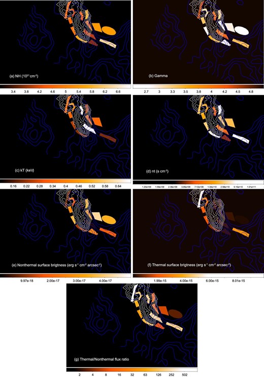
Parameter maps of the spectral fitting: (a) absorption column, (b) photon index, (c) temperature, (d) ionization timescale, (e) nonthermal X-ray surface brightness in the 2–10 keV band in units of erg s−1 cm−2 arcsec−2, (f) thermal X-ray surface brightness in the 0.5–10 keV band in units of erg s−1 cm−2 arcsec−2, and (g) flux ratio between thermal and nonthermal emission. The color scales are linear for (a), (b), (c), (e), and (f) and logarithmic for (d) and (g). For (c) and (d), we have no data for the src2 region. White and blue contours represent the 12CO and H i distribution, as in figures 1 and 2, respectively.
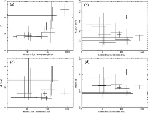
Correlation plot between the flux ratio of the thermal and nonthermal components and the photon index of nonthermal emission (a), NH (b), kTe (c), and net (d).
On the other hand, the thermal parameters, kT (figure 5c) and nt (figure 5d), show no clear tendency in the correlation with dense clouds. The correlation plot shown in figures 6b–d also supports this lack of clear correlation.
4 Discussion
We carried out spatially resolved spectroscopy and found that filaments interacting with the dense cloud have enhanced thermal emission, and fainter and possibly softer synchrotron X-rays. The absorption column in the cloud regions is rather small, which may imply that the cloud is on the rear side of the remnant.
The apparent positive correlation between the flux ratio of thermal and nonthermal X-rays and the photon index of nonthermal X-rays shown in figure 6a could be mainly due to a deceleration of the shock velocity caused by the interaction of the shock with dense material. In the synchrotron loss-limit regime, the roll-off energy of the synchrotron X-rays is proportional to the square of the shock velocity (Aharonian & Atoyan 1999; Yamazaki et al. 2006; Zirakashvili & Aharonian 2007). Thus the interacting shocks should have smaller shock velocity, and softer (and as a result fainter) synchrotron X-rays. The thermal X-rays are enhanced by the shock compression, which results in bright soft X-ray filaments around the clouds. We thus conclude that this region of RCW 86 well follows the synchrotron loss-limit regime.
The enhancement of thermal X-rays and fainter and softer synchrotron X-ray emission is also shown in the interacting regions of several SNRs, such as the north-western rim (Bamba et al. 2008; Sano et al. 2022) of SN 1006 and Tycho (Lopez et al. 2015). In most SNRs bright X-ray synchrotron emission also appears to coincide with no or very faint thermal X-ray emission (e.g., Nakamura et al. 2012). These facts all imply that the bright synchrotron X-rays are emitted around non-interacting, fast shocks. Our results for RCW 86 show such thermal X-ray enhancement and decline of synchrotron X-rays in the interacting regions with smaller spatial scales, 1″ or 0.7 pc at a 2.3 kpc distance, compared with previous results with spatial scales larger than a few pc.
On the other hand, our result is in contrast to the case of RX J1713.7−3946 (Sano et al. 2013), where synchrotron X-rays are enhanced around the shock–cloud interacting regions. Similarity to RX J1713−3946 is also observed in Kepler; Sapienza et al. (2022) revealed that the acceleration efficiency in Kepler is higher in the northern interacting region with the shock and circumsteller medium, compared with the south of the remnant. In the same remnant, RCW 86, Suzuki et al. (2022) showed that thermal and synchrotron X-rays are enhanced in the denser region. Inoue et al. (2012) suggest that such a tendency happens when shocks collide with clumpy clouds; when the shock runs into clumpy medium, the dense clumps can survive in the shock downstream region without evaporation and amplify the downstream magnetic field, which causes enhanced synchrotron X-rays (see also Sano & Fukui 2021).
This scenario may indicate that the difference between the shock–cloud interacting regions in RCW 86 and RX J1713.7−3946 may be a result of the different shock environments. In RX J1713.7−3946, the intercloud density is ∼0.01–0.1 cm−3 (Weaver et al. 1977; Cassam-Chenaï et al. 2004; Katsuda et al. 2015). Sano et al. (2020) discovered shocked cloudlets with a density of ∼104 cm−3; thus the clumpiness, the density contrast between dense clouds and intercloud regions, should be high. This is consistent with the calculation by Celli et al. (2019). On the other hand, the density contrast between clouds and intercloud medium surrounding RCW 86’s eastern region could be smaller, since the dense cloud detected in 12CO is covered by less dense intercloud medium, which is detected with H i emission. The cloud interacting with SN 1006 is also detected by H i observation only (Sano et al. 2022), implying a less clumpy interstellar medium. A similar discussion is given by Sano and Fukui (2021). On the interaction between the shock and such dense and rather uniform clouds, the shock-heated plasma can emit strong thermal bremsstrahlung, which should be the cause of the bright thermal filaments that we observed. In order to test our scenario, we need high-spatial-resolution CO and H i observations of RCW 86 to compare the south-west (RX J1713-like) and eastern (SN 1006-like) regions to see if there are high-density clouds, and whether density contrast causes synchrotron X-ray enhancement.
In this study, we found no significant variation of temperature and ionization timescale for the thermal emission. This is mainly due to the lack of energy resolution and statistics, leading to large error ranges. Future X-ray missions with excellent energy resolution, such as XRISM (Tashiro et al. 2020) and Athena (Nandra et al. 2013), will resolve this issue.
5 Summary
Spatially resolved spectroscopy of the south-eastern region of the young supernova remnant RCW 86 is carried out with deep XMM–Newton observations. It is found that soft thermal X-rays are enhanced on the edges of dense clouds, detected with 12CO or H i observations. These regions show fainter and possibly softer nonthermal X-rays from accelerated electrons. These results indicate that the shock decelerates due to the interaction with clouds, causing thermal X-ray enhancement due to the density increase and fainter and softer synchrotron X-rays due to the smaller shock speed. Our results indicate that the dense region does not enhance synchrotron X-rays, in agreement with the suggestions by Aharonian and Atoyan (1999), Yamazaki et al. (2006), and Zirakashvili and Aharonian (2007). No synchrotron X-ray enhancement in the shock–cloud interaction region is found in this region. This is similar to SN 1006 and Tycho, and in contrast to RX J1713.7−3946. This difference could be due to differences in the surrrounding environment, such as the high density contrast of surrounding material. For further study of the effect of surrounding material on synchrotron X-ray enhancement, we need follow-up observations with ALMA to study the density contrast of surrounding material of RCW 86, and XRISM/Athena observations to measure the precise parameters of thermal emission to understand the thermal conditions.
Acknowledgments
We thank the anonymous referee for his/her productive comments. We thank Hiromichi Okon and Yukikatsu Terada who helped us to make the parameter maps. This work was financially supported by Japan Society for the Promotion of Science Grants-in-Aid for Scientific Research (KAKENHI) Grant Numbers JP19K03908 (AB), JP23H01211 (AB), 20KK0309 (HS), 21H01136 (HS), 22H01251 (RY), and 23H04899 (RY).
