


Abstract
We propose a new evolutionary process for protoplanetary disks, the co-evolution of dust grains and protoplanetary disks, revealed by dust–gas two-fluid non-ideal magnetohydrodynamics simulations considering the growth of dust grains and associated changes in magnetic resistivity. We found that the dust growth significantly affects disk evolution by changing the coupling between the gas and the magnetic field. Moreover, once the dust grains grow sufficiently large and the adsorption of charged particles on to them becomes negligible, the physical quantities (e.g., density and magnetic field) of the disk are well described by characteristic power laws. In this disk structure, the radial profile of density is steeper and the disk mass is smaller than those of the model ignoring dust growth. We analytically derive these power laws from the basic equations of non-ideal magnetohydrodynamics. The analytical power laws are determined only by observable physical quantities, e.g., central stellar mass and mass accretion rate, and do not include difficult-to-determine parameters, e.g., the viscous parameter α. Therefore, our model is observationally testable and this disk structure is expected to provide a new perspective for future studies on protostar and disk evolution.
1 Introduction
In protoplanetary disks, dust grains are not only the building blocks of the planets, but also play a key role in determining the ionization degree of the disk gas by adsorbing charged particles (ions and electrons) in the gas phase. Since the ionization degree determines the magnetic resistivity, i.e., the degree of coupling between the gas and magnetic field, the microscopic nature (|${\mu } {\rm m}$| to cm scale) of the dust grains is expected to influence the macroscopic disk evolution (100 au, i.e., 1015 cm scale) via magnetic resistivity (Zhao et al. 2016; Guillet et al. 2020; Marchand et al. 2020; Tsukamoto & Okuzumi 2022).
Previous studies have shown that non-ideal magnetohydrodynamics (MHD) effects arising from finite resistivity, specifically ambipolar diffusion, dramatically weaken the coupling between the magnetic field and gas, thereby enabling the formation of a disk (Tomida et al. 2015; Tsukamoto et al. 2015; Masson et al. 2016; Wurster et al. 2016). Moreover, ambipolar diffusion determines the magnetic flux evolution in protostars (Li 1998; Tsukamoto et al. 2020).
Previous studies on the formation and evolution of protoplanetary disks assumed that dust grains possess the properties (such as the size distribution) of the interstellar medium (ISM) dust grains. However, in the disk, the dust growth timescale is ∼104 yr, which is much shorter than the lifetime of the disks (∼106 yr). Thus, it is unsatisfactory to study disk evolution with resistivity assuming ISM dust (Tsukamoto et al. 2022).
How would the dust growth affect the ionization degree? As dust grains merge and grow, their total surface area decreases. Therefore, the adsorption of charged particles by dust grains becomes ineffective, and the gas-phase ionization degree is expected to increase and magnetic resistivity to decrease accordingly. Recent studies on dust growth and associated changes in magnetic resistivity have shown a decrease in magnetic resistivity (Zhao et al. 2016; Guillet et al. 2020; Marchand et al. 2020; Kawasaki et al. 2022; Tsukamoto & Okuzumi 2022), and some studies have also shown changes in gas dynamics as a result (Lebreuilly et al. 2023; Marchand et al. 2023).
However, the effect of dust growth on the evolution of the protoplanetary disk is still unclear, because the calculations in the aforementioned studies were performed assuming spherical symmetry (Lebreuilly et al. 2023) or 3D simulation up to the prestellar or first core formation stage in which the gas is supported by the pressure gradient force (Marchand et al. 2023).
In this study, we report simulation results of the formation and evolution of protoplanetary disks ∼104 yr after the formation of protostars considering dust growth inside the disk, the associated change of magnetic resistivity, and its feedback on the disk dynamics. Moreover, we present an analytical argument that explains the resulting disk structures. Based on these results, we propose a new evolutionary process for protostars: co-evolution of dust grains and protoplanetary disks.
2 Methods and initial conditions
2.1 Numerical methods
2.1.1 Two-fluid magnetohydrodynamics simulations
We solve two-fluid magnetohydrodynamics equations for the dust–gas mixture. The governing equations are given as
where ρ[g, d] denotes the mass densities and the subscripts [g, d] denote the gas and dust components, respectively. ρ = ρg + ρd denotes the total density. |$\epsilon$| = ρd|$/$|ρ denotes the dust-to-total-mass ratio, v = (ρgvg + ρdvd)|$/$|(ρg + ρd) denotes the barycentric velocity of the dust–gas mixture where v[g, d] denotes the gas and dust velocity, Δv = (vd − vg) denotes the the velocity difference between gas and dust, and P denotes the gas pressure. J denotes the electric current. c denotes the speed of light. ηO and ηA denote the ohmic and ambipolar resistivities, respectively. The details of the approximations adopted in the governing equations and numerical method are described in Tsukamoto, Machida, and Inutsuka (2021a). Our numerical simulations consider the ohmic and ambipolar diffusions, but ignore the Hall effect.
We adopt a barotropic equation of state (EOS) in which the gas pressure depends only on the density:
cs, ref = 190 m s−1 is the isothermal sound velocity at 10 K. We used a critical density of ρc = 4 × 10⁻¹⁴ g cm−3, above which gas behaves adiabatically, and ρe = 10−11 g cm−3, above which gas behaves as diatomic molecule. In our simulations, the gas density is in the range of ρg < 10−9 g cm−3 and ignoring the dissociation of H2 in the equation of state does not affect the results.
2.1.2 Dust growth
We consider dust growth with a single-size approximation (Sato et al. 2016; Okuzumi et al. 2016; Tsukamoto et al. 2017). The governing equation of dust growth is
where ad denotes the representative dust size, |$t_{\rm growth}=1/(\pi a_{\rm d}^2 n_{\rm d} \Delta v_{\rm dust})$|, nd denotes the dust number density, Δvdust denotes the collision velocity between the dust grains, Dd|$/$|Dt = ∂|$/$|∂t + vd · ∇, and
which models the collisional mass gain and loss (Okuzumi et al. 2016). We assume vfrag = 30 m s−1. For the dust relative velocity Δvdust, we consider the sub-grid scale turbulence and Brownian motion.
For the turbulent-induced dust relative velocity Δvturb, we adopt the prescription presented by Ormel and Cuzzi (2007),
where |$\delta v_{\rm Kol}=Re_L^{-1/4}$| and |$t_{\rm Kol}=Re_L^{-1/2} t_L$| denote the eddy velocity and eddy turn-over timescale at dissipation scale and ReL = LvL|$/$|ν denotes the Reynolds number. We set the stopping time tstop,1 = tstop(ad) and tstop,2 = 1|$/$|2 tstop(ad) referring to Sato, Okuzumi, and Ida (2016), where tstop(ad) is calculated as in our previous study (Tsukamoto et al. 2021a).
We assume sub-grid turbulence of the “α turbulence model” (Tsukamoto et al. 2021b), in which we assume
αturb = 2 × 10⁻³ denotes the dimensionless parameter that determines the strength of the sub-grid turbulence and ag denotes the gravitational acceleration: see Tsukamoto, Machida, and Inutsuka (2021b) for the underlying physical assumptions for this turbulence model. αturb is hard to determine from simulations, although it does not affect the dust growth timescale as strongly as density. In this paper, we adopted this fixed value just for simplicity. Larger (smaller) αturb values decrease (increase) the dust growth timescale.
2.1.3 Resistivity calculations
For the resistivity model, we adopt the analytical resistivity formula described in Tsukamoto and Okuzumi (2022) in which we analytically solve the equations for chemical equilibrium in the gas phase and detailed balance equations for dust charging. The dust size distribution considered in resistivity calculations is set to be
where A denotes a constant for normalization. Here we assume that the maximum dust size is amax = ad of equation (7) (which is valid when q < 4). The minimum dust size amin and power exponent q are the parameters of this study.
The temperature for the resistivity calculation is calculated according to the equation of state (6).
Our resistivity model does not include charge neutralization due to grain–grain collisions because the dust grains tend to coalesce and grow rather than bounce when (sub-)micron-sized small dust particles collide (Dominik & Tielens 1997; Blum et al. 2000; Weidling et al. 2012; Gundlach & Blum 2015). Note also that the grain–grain neutralization is important for resistivities only when there are significant amounts of small dust grains and they contribute to the electric current. Since we are interested in the impact of dust growth and in the situations in which the contribution of the dust grains becomes minor, neglecting grain–grain neutralization does not change our main claims in this paper. See Tsukamoto and Okuzumi (2022) for more discussions.
2.1.4 Sink particle
A sink particle is dynamically introduced when the density exceeds ρsink = 10−12 g cm−3. The sink particle absorbs smoothed-particle hydrodynamics (SPH) particles within rsink < 1 au.
2.2 Initial conditions
We adopt the density-enhanced Bonnor–Ebert sphere, which is surrounded by a medium with a steep density profile used by Tsukamoto, Machida, and Inutsuka (2021b) as a initial condition.
The radius of the core is Rc = 4.8 × 10³ au and the enclosed mass within Rc is Mc = 1 M⊙. We adopt an angular velocity profile of Ω(d) = Ω0|$/$|(exp {10[d|$/$|(1.5 Rc)] − 1} + 1) with |$d=\sqrt{x^2+y^2}$| and Ω0 = 2.3 × 10⁻¹³ s−1. We assume a constant magnetic field |$(B_x,B_y,B_z)=(0,0,50\, \mu \mathrm{G})$|.
The parameter αtherm (≡ Etherm|$/$|Egrav) is 0.4, where Etherm and Egrav denote the thermal and gravitational energies of the central core (without surrounding medium), respectively. The parameter βrot (≡ Erot|$/$|Egrav) within the core is 0.03, where Erot denotes the rotational energy of the core. The mass-to-flux ratio of the core normalized by the critical value is μ|$/$|μcrit = 5.
We adopt a dust density profile of ρd(r) = fdgρg(r)|$/$|(exp {10[r|$/$|(1.5Rc)] − 1} + 1), where fdg = 10−2 denotes the dust-to-gas mass ratio. The dust density profile has the same shape as the gas density profile in r ≲ 1.5 Rc but is truncated at r ≥ 1.5Rc. The initial (maximum) dust size is assumed to be |$a_{\rm d}=0.1 \, {\mu } {\rm m}$|.
We resolve 1 M⊙ with 3 × 10⁶ SPH particles. The names and parameters of the models are listed in table 1.
Names and parameters of the models.*
| Model name | amin [nm] | q | ζCR [s−1] | Dust growth |
|---|---|---|---|---|
| ModelA100Q25 | 100 | 2.5 | 10−17 | Y |
| ModelA100Q35 | 100 | 3.5 | 10−17 | Y |
| ModelA5Q25 | 5 | 2.5 | 10−17 | Y |
| ModelA5Q35 | 5 | 3.5 | 10−17 | Y |
| ModelZeta18 | 100 | 2.5 | 10−18 | Y |
| ModelA100Fixed | 100 | — | 10−17 | N |
Model name, minimum dust size amin, power exponent for dust size distribution q, and cosmic ray ionization rate ζCR. “Y” means that the dust growth is considered in the simulation and “N” means that the dust growth is not considered.
3 Results
3.1 Co-evolution of dust grains and protoplanetary disks
Figure 1 shows the time evolution of (a) density, (b) total magnetic resistivity (ηO + ηA), (c) dust size, and (d) plasma β in our fiducial model, ModelA100Q25. Panel 1-a shows the formation of a disk with a size of ∼20 au at t* = 1.1 × 10³ yr (where t* denotes the time after protostar formation). At this stage, the total magnetic resistivity is ∼1019 cm2 s−1 and relatively large (panel 1-b). This large value is attributed to the fact that the maximum dust size remains |$a_{\rm d}<1 \, {\mu } {\rm m}$| within the disk (panel 1-c) and dust adsorption of charged particles is effective. Owing to the efficient magnetic diffusion, the plasma β inside the disk is significantly high (panel 1-d).
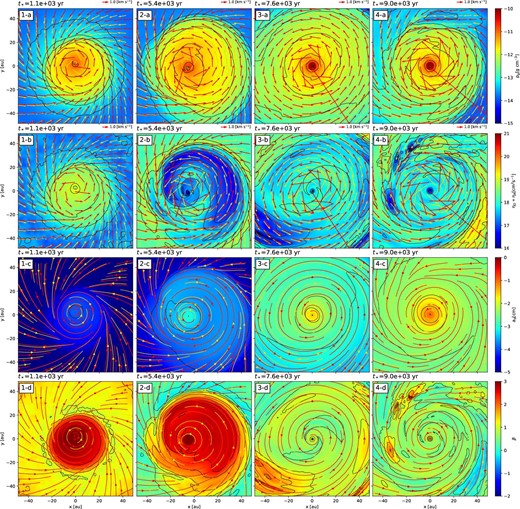
Time evolution of the (a) gas density, (b) magnetic resistivity (ηO + ηA), (c) dust size (ad), and (d) plasma β on the x–y plane with a box of 100 au. The time after protostar formation is shown in the upper left. The red and orange arrows show the velocity field of the dust and gas, respectively, on the x–y plane. The red and orange lines show their respective streamlines. The black lines are the contours of the quantity of each panel. The contour levels are (a) ρg = 10−15, 10−14.5, …, 10−10 g cm−3, (b) ηO + ηA = 1016, 1016.5, …, 1021 cm2 s−1, (c) ad = 10−5, 10−4.5, …, 100 cm, and (d) β = 10−2, 10−1.5, …, 103.
As the time progresses, a remarkable change in the magnetic resistivity occurs. Panel 2-b shows a significant decrease in the magnetic resistivity within the disk. This is caused by dust growth within the disk (ad reaches |$10 \, {\mu } {\rm m}$|) and a reduction in the dust adsorption efficiency: see appendix 2 and Tsukamoto and Okuzumi (2022) for the impact of dust size on the ambipolar resistivity. However, at this epoch, the decrease in the magnetic diffusion efficiency does not lead to a decrease in the disk size; instead, the disk continues to expand. The plasma β also remains high.
The decrease in the magnetic resistivity leads to better coupling between the magnetic field and gas in the disk. This coupling promotes gas accretion, which in turn transports the magnetic flux to the center and reduces the plasma β in the disk (panel 3-d). The increase of the magnetic field amplifies the magnetic resistivity (ηA) in the central region (panel 3-b). Once the dust grows sufficiently, ηA is proportional to the square of the magnetic field strength even inside the disk. Even at this point, the gas density map (panel 3-a) indicates the presence of a relatively large disk of ∼50 au.
The strong magnetic field in the disk causes efficient magnetic braking and efficient mass accretion over the entire disk, leading to a decrease in the disk size from panels 3-a to 4-a. However, the density structure of the central region is very similar in panels 3-a and 4-a. On the other hand, between panels 2-a and 4-a, the disk size is similar, but the density structure of the inner region is different. This indicates that the inner disk structure transits from panels 2-a to 3-a as the dust grains grow.
In this way, the growth of the dust grains causes a decrease in the magnetic resistivity and changes the magnetic activity of the disk, ultimately determining the evolution of the disk. Conversely, changes in the disk structures affect the dust growth in the disk (see figure 7 below). Based on these results, we propose a new evolutionary process for the protoplanetary disk: co-evolution of dust grains and protoplanetary disks.
3.2 Radial disk structure and comparison with analytical solutions
Figure 2 shows the azimuthally averaged radial profiles at the midplane of ModelA100Q25. The red, orange, magenta, and green lines show profiles at the epochs of panels 1–4 in figure 1, respectively.
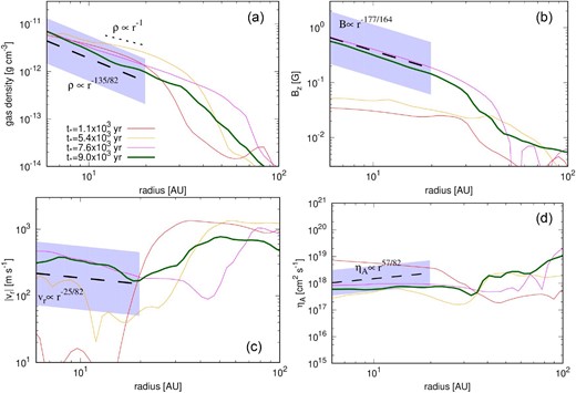
Time evolution of the azimuthally averaged radial profile of (a) gas density, (b) vertical magnetic field, (c) radial velocity, and (d) ambipolar resistivity (ηA). The epoch of each line is the same as in figure 1. The black dashed lines indicate the analytical solutions (A45)–(A49) in which the following values, ρc = 4 × 10⁻¹⁴ g cm−3, ζCR = 10−17s−1, cs, ref = 190 m s−1, |${M}^{^{^{{.}}}}$| |$=2\times 10^{-5}$| M⊙ yr−1, and M = 0.3 M⊙, are assumed. The hatched areas are regions within a factor of three from the solutions.
In the early evolutionary phase when the dust size is sufficiently small (t* ≲ 5 × 10³ yr; red and orange lines), the gas density has a relatively shallow profile with the power of |$D_{\rho _{\rm g}} \sim -1$| [red and orange lines; where Df denotes the power exponent of a quantity f as |$f(r) \propto r^{D_f}$|]. As the dust grains grow, the gas density profile becomes steeper and appears to converge to a power law with |$D_{\rho _{\rm g}} \sim -2$| (at t* = 9 × 10³ yr; green line).
To explain this disk structure, we analytically derive the new steady-state solutions of the disk in appendix 1. The important assumptions in deriving the steady-state solutions are that (1) the magnetic braking determines the disk angular momentum evolution (and angular momentum transfer by the viscosity is negligible), (2) radial magnetic flux transport is determined by the balance between gas advection and ambipolar diffusion, and (3) the adsorption of charged particles on the dust grains is negligible and the ionization degree is determined by cosmic ray ionization and gas phase recombination (for the details of the derivation, see appendix 1).
The derived solution of the density profile predicts |$D_{\rho _{\rm g}} = -\frac{135}{82}$| [equation (A45)]. The black dotted line and hatched areas indicate the analytical solutions and a region within a factor of three of the solution, respectively. Here, we have chosen the following values for the analytical solution: ρc = 4 × 10⁻¹⁴ g cm−3, ζCR = 10−17 s−1, cs, ref = 190 m s−1, which come from the simulation setup, and |$\dot{M}=2\times 10^{-5} \, M_{\odot} \,{\rm yr}^{-1}$| and M = 0.3 M⊙, to be approximately consistent with the values at t* = 9 × 10³ yr. Our analytical solution well agrees with the simulation result not only in terms of the power, but also in terms of the exact value.
Panel (b) shows that, in the early evolutionary phase (red and orange lines), the magnetic field in the disk is almost constant (|$D_{B_z} \sim 0$|), which is in agreement with previous studies (Tsukamoto et al. 2015; Masson et al. 2016) in which the dust growth is ignored. In contrast, as the dust grains grow, the vertical magnetic field profile becomes steeper and converges to a power law with |$D_{B_z} \sim -1$|. Our analytical solution suggests the power exponent of |$D_{B_z} = -\frac{177}{164}$| [equation (A46)] and agrees with the simulation results at t* = 9.0 × 10³ yr (green line). The black dotted line indicates our analytical solution with the same parameters used in the density profile and the hatched area is a region within a factor of three from the solution. The black dotted line confirms that our analytical solution simultaneously reproduces the density and magnetic field with a single set of parameters and quantitatively agrees with the simulation results.
Panel (c) shows that, when the dust size is small, the absolute value of the radial velocity is |vr| ≲ 10 m s−1 (red line). As the dust grows, it increases in the order of 100 m s−1. The proposed analytical solution suggests a power of |$D_{v_r} = -\frac{25}{82}$| and a value of ∼100 m s−1. Although vr possesses relatively strong time fluctuation, the simulation results at t* = 9.0 × 10³ yr (green line) agree with the analytical solutions.
Panel (d) shows that the ηA profile in the simulation is almost radially constant once the dust grains grow sufficiently large (magenta and green lines). On the other hand, our analytical model predicts a slightly positive power law with |$D_{\eta _A}=\frac{57}{82}$|. Compared to the other physical quantities, the difference between the simulation result and the analytical solution is relatively large, but still within a factor of three in the region r ≲ 10 au.
3.3 Diversity and universality of disk evolution
As seen in the previous section, the disk evolution is significantly affected by the dust growth. Furthermore, once the dust grains grow sufficiently large, the disk structure of our fiducial model is well described by the power laws analytically derived in appendix 1. In this section, we examine the impact of the minimum dust size and dust power exponent on the evolution of the disk. Moreover, we examine the effect of the cosmic ray ionization rate. Through these considerations, we discuss the diversity and universality of protoplanetary disk evolution.
Before discussing the simulation results, we summarize how the minimum dust size amin and the power exponent q affect the magnetic resistivity based on our previous studies (Tsukamoto & Okuzumi 2022). Figures that show how the resistivities depend on amax with various q and amin can be found in Tsukamoto and Okuzumi (2022).
The adsorption of dust grains, which plays the primary role in determining the resistivity, depends on the dust total cross-section, which depends on q and amin. In cases in which q is less than 3, the maximum dust size determines the total surface area. Conversely, in cases in which q is larger than 3, both the maximum and minimum dust sizes affect the total surface area. Consequently, when q is large (or the size distribution is steep), the influence of dust growth tends to be weaker.
Another important factor that influences resistivity is conductivity generated by the dust grains. If a significant amount of dust with a size of ≲10 nm is present, the dust grains contribute to the conductivity. In such cases, resistivity at a high density is smaller than that when the minimum size is, for instance, 100 nm. This effect is pronounced in cases in which the dust grains have not grown and the size distribution is steep (i.e., q is large).
3.3.1 Comparison of density structures
Figure 3 shows a density map of all models. Although the disk size differs among the simulations, the density structures of the inner ∼20 au region of panels (a) ModelA100Q25, (b) ModelA100Q35, (c) ModelA5Q25, and (f) ModelZeta18 are very similar. In these simulations, the inner density structures are consistent with the analytical solutions. The spiral patterns in the outer regions of the disks are created by gravitational instability. We confirm that Toomre’s Q parameter values in these regions are Q ∼ 1 in the outer regions of these disks.
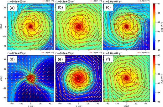
Gas density map of (a) ModelA100Q25, (b) ModelA100Q35, (c) ModelA5Q25, (d) ModelA5Q35, (e) ModelA100Fixed, and (f) ModelZeta18 on the x–y plane. The time after protostar formation is shown in the upper left. The red and orange arrows show the velocity field of the dust and gas, respectively, on the x–y plane. The black lines indicate the density contour. The contour levels are ρg = 10−15, 10−14.5, …, 10−10 g cm−3.
On the other hand, figure 3d (ModelA5Q35) shows the formation of a very small disk of ≲10 au and bubble-like structures around it. These bubble-like structures are created by magnetic interchange instability (Krasnopolsky et al. 2012). The large amounts of small dust grains make ambipolar diffusion (and ohmic diffusion) ineffective in the high-density region and lead to the development of interchange instability as a redistribution mechanism of magnetic flux.
Figure 3e (ModelA100Fixed) in which the dust growth is artificially ignored shows that the disk is relatively compact, dense, and massive. This massive disk is consistent with previous theoretical studies; however, such a massive disk seems to be inconsistent with the observations (Tsukamoto et al. 2022).
3.3.2 Universality of the disk structure
Figure 4 shows the azimuthally averaged radial profiles of all models. The dashed lines show the power laws of our analytical solutions (in this figure, we plot the power laws just as a reference because parameters such as central star mass or mass accretion rate differ among the models).
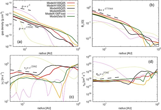
Azimuthally averaged radial profile of (a) gas density, (b) vertical magnetic field, (c) radial velocity, and (d) ambipolar resistivity (ηA). The red, orange, black, yellow, magenta, and green lines show the results of ModelA100Q25, ModelA100Q35, ModelA5Q25, ModelA5Q35, ModelA100Fixed, and ModelZeta18, respectively. The thick lines show the models that are in good agreement with the power laws of the analytical solution. The time of each line is the same as in figure 3. The black dashed lines indicate the power laws of the analytical solutions.
Of the five models that consider dust growth, four models have an inner region of ∼20 au consistent with the analytical solution (red, green, black, and orange lines). If we regard the disk radius as the radius at which the density distribution deviates from the power law of the analytical solution, ModelZeta18 has the largest disk size, and ModelA100Q35, ModelA100Q25, and ModelA5Q25 have smaller disk sizes in this order (see also figure 5). This difference may be due to the difference in resistivity in the regions where dust grains have not grown (outer region of the disk and envelope). Despite the difference in disk size, the universality of the disk structure in the inner region is noteworthy.
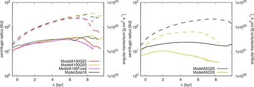
Time evolution of centrifugal radius (solid lines and left axis) and total angular momentum of the disk (dashed lines and right axis). Red, orange, black, yellow, magenta, and green lines show the results of ModelA100Q25, ModelA100Q35, ModelA5Q25, ModelA5Q35, ModelA100Fixed, and ModelZeta18, respectively. The horizontal axis shows the time after protostar formation.
Note that the disk structure of ModelZeta18 (green lines) is more consistent with the power laws of the analytical solutions than the fiducial model. For example, ηA has a positive power exponent. This is because this model is more evolved than the fiducial model and the approximation on ηA in the analytical solution is better validated.
Figure 4 shows that the disk of ModelA5Q25 (yellow) is very small and has a different structure from the other four models. A large amount of small dust in this model makes ambipolar diffusion ineffective from the beginning of disk formation in the high-density region. The disk rapidly shrinks before the dust grows and ηA is well described by the analytical form of Shu (1983). Thus, the disk evolution of the model is different from other models.
It would be instructive to see the differences in disk structure between the model ignoring the dust growth (ModelA100Fixed; magenta) and those that are well described by the analytical solutions. In the model without the dust growth, the density and ηA are large and the magnetic field and radial velocity vr are small. This is because, in the absence of the dust growth, the ambipolar diffusion in the disk is extremely effective. It suppresses magnetic braking in the disk, resulting in smaller vr and an increased density due to gas accumulation in the disk. Furthermore, the magnetic flux is extracted from the disk by ambipolar diffusion, causing the low value of the disk magnetic field. The density of the disk in ModelA100Fixed is large and Toomre’s Q parameter is Q ∼ 1 even in the inner region.
3.4 Time evolution
In this section, we examine the time evolution of disk angular momentum (and radius), disk mass, typical dust size and dust abundance in disks. We also investigate the mass ejection rate by outflows from the disks.
3.4.1 Time evolution of the disk size
Figure 5 shows the time evolution of centrifugal radius and the angular momentum of the disk. The angular momentum of the disk J(ρdisk) is calculated as
For the density threshold of the disk, we choose ρdisk = 10−13 g cm−3. The centrifugal radius is calculated as
Here |$\bar{j}(\rho _{\rm disk})=J(\rho _{\rm disk})/M_{\rm disk}$|, where Mdisk denotes the enclosed gas mass within the region ρg > ρdisk. Comparing the radius of the region with a density of ρg > ρdisk (figure 4) with the centrifugal radius, the former is about twice as large as the latter owing to the radial density distribution and temporal density oscillation by the non-axisymmetric structures. In this study, we consider the centrifugal radius as an estimate of the disk size.
The left panel of figure 5 shows the results of the models with amin = 100 nm. In ModelA100Q25 (red line), the angular momentum of the disk continues to increase until t* ∼ 7 × 10³ yr, and then it shows a sharp decrease. This is because the dust grains grow to |$a_{\rm d}\gtrsim 10 \, {\mu } {\rm m}$| (see figure 7 below), which causes a sudden decrease in magnetic resistivity and the extraction of angular momentum by the magnetic field. Interestingly, although the angular momentum has decreased by a factor of ∼1|$/$|3 from t* ∼ 7 × 10³ yr to t* ∼ 9 × 10³ yr, the centrifugal radius has decreased by only a factor of ∼1|$/$|2. This indicates that the disk mass also decreases rapidly during this period (figure 6). For ModelA100Q35, no such rapid decrease of angular momentum is observed. This is because amin is also responsible for the total dust surface area, and thus the decrease in magnetic resistivity is not so drastic (Tsukamoto & Okuzumi 2022). As exhibited by ModelZeta18 (green line), the low cosmic ray ionization rate can contribute to maintaining the angular momentum. This is in agreement with previous studies (Wurster et al. 2018; Kuffmeier et al. 2020; Kobayashi et al. 2023). The decrease in the disk size of ModelA100Fixed is caused by the pseudo-disk warp and associated inward magnetic flux drag (Tsukamoto et al. 2020). In this model, the angular momentum decreases by less than a factor of two, which is not significant compared to ModelA100Q25.
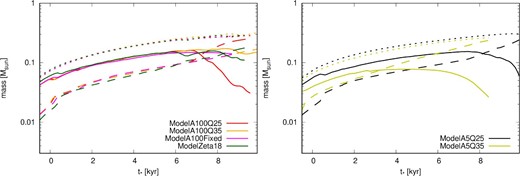
Time evolution of the mass of the disks (solid lines), the protostars (dashed lines), and the total mass (dotted lines). Red, orange, black, yellow, magenta, and green lines show the results of ModelA100Q25, ModelA100Q35, ModelA5Q25, ModelA5Q35, ModelA100Fixed, and ModelZeta18, respectively. The horizontal axis shows the time after protostar formation.
The right panel of figure 5 shows the results of the models with amin = 5 nm. Interestingly, the relationship between the disk size and power exponent q is different from the models with amin = 100 nm. The disk size of the model with q = 3.5 (ModelA5Q35) is significantly smaller than that in the model with q = 2.5 (ModelA5Q25). This is because, when there is a large amount of small dust (∼nm), the dust grains are responsible for the conductivity and reduce the magnetic resistivity. This allows magnetic braking to work more effectively in ModelA5Q35 and reduce the disk size.
3.4.2 Time evolution of the disk mass
Figure 6 shows the time evolution of disk mass Mdisk (solid), protostar mass Mstar (dashed), and total mass Mstar + Mdisk (dotted). In ModelA100Q25 (red), the disk mass continues to increase and reaches ∼0.15 M⊙ at t* ∼ 7 × 10³ yr. Then, it drops sharply to Mdisk ∼ 0.03 M⊙ at t* ∼ 9 × 10³ yr. Meanwhile, mass accretion on to protostars is enhanced and the protostellar mass rapidly increases from 0.1 M⊙ to 0.2 M⊙ in this period, giving a mass accretion rate of ≳10−5 M⊙ yr−1 for this model. In ModelZeta18 (green line) and ModelA5Q25 (black line), it appears that the disk mass also begins to decrease towards the end of the simulations. However, the time at which the decrease begins is later than in ModelA100Q25.
In ModelA100Fixed, the disk radius decreases in t* ≳ 6 × 10³ yr (figure 5) but the disk mass does not significantly change. This suggests that the disk evolution without dust growth is different from the models that include dust growth and that are consistent with the analytic solution. In ModelA5Q35, the mass (and radius) evolution differs from the other models. This is due to inefficient ambipolar diffusion since disk formation. Thus, the situation close to the ideal MHD is realized.
3.4.3 Time evolution of dust size and dust abundance in the disk
Figure 7 shows the time evolution of the dust-to-gas mass ratio and mean dust size of the disks. The dust mass and mean dust size of the disk is calculated as
and
respectively.
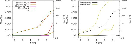
Time evolution of the dust-to-gas mass ratio (solid lines and left axis) and mean dust size in the disk (dashed lines and right axis). Red, orange, black, yellow, magenta, and green lines show the results of ModelA100Q25, ModelA100Q35, ModelA5Q25, ModelA5Q35, ModelA100Fixed, and ModelZeta18, respectively. The horizontal axis shows the time after protostar formation.
The figure shows that the increase in the dust-to-gas mass ratio occurs later in the simulation. This increase begins when the average dust size in the disk exceeds |${\sim }100 \, {\mu } {\rm m}$|. This is due to the “ash-fall” phenomenon proposed in our previous study (Tsukamoto et al. 2021b). The largest increase is observed in ModelA100Q25, where the dust-to-gas mass ratio increases to 1.04% at the end of the simulation. Some readers may think that this value is small and irrelevant. However, we only considered ∼103 yr after the ratio started to increase. If this event continues for, for instance, 105 yr (i.e., during the Class 0/I phase), it can cause a significant increase in the dust abundance.
The increase of the dust-to-gas mass ratio is slower in ModelA100Q35, ModelA5Q25, and ModelZeta18 compared to ModelA100Q25 owing to the lower outflow activity (i.e., weaker coupling between the magnetic field and gas in the upper layers of the disk; figure 8) in these models.
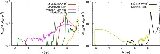
Time evolution of the mass ejection rate. Red, orange, black, yellow, magenta, and green lines show the results of ModelA100Q25, ModelA100Q35, ModelA5Q25, ModelA5Q35, ModelA100Fixed, and ModelZeta18, respectively. The horizontal axis shows the time after protostar formation.
3.4.4 Time evolution of the mass ejection rate by outflow
Figure 8 shows the time evolution of the mass ejection rate due to the molecular outflow. The mass ejection rate is calculated as
where |$v_r^+ \equiv \max (\mathbf {v}\cdot \mathbf {r},0)$| denotes the positive radial velocity, and we perform the surface integral on a sphere with a radius of 100 au.
The mass ejection rate is highly variable and has a peak value of ≳10−5 M⊙ yr−1. This is comparable to the mass accretion rate in the disk. Figures 7 and 8 suggest that a mass ejection rate of 10−6 to 10−5 M⊙ yr−1 and a mean dust size of |${\sim }100 \, {\mu } {\rm m}$| are required for the “ash-fall” phenomenon to happen, in which the disk gas is selectively ejected into interstellar space by the outflow and the dust grains are resupplied to the disk.
4 Discussion
4.1 Universality of the disk structure in a disk with grown dust grains
In this study, we propose a new disk evolutionary picture, the co-evolution of dust grains and protoplanetary disks based on non-ideal dust–gas two-fluid MHD simulations considering dust growth. The dust growth changes the gas-phase ionization degree, magnetic resistivity, and evolution of the disk. In the co-evolution process, microscopic dust grains of micrometer size couple with macroscopic disks of 100 au size and they co-evolve. The size scale difference between two objects is 1019, which is astounding compared to the well-known co-evolution of super massive black holes and galaxies (where the size scale difference is ∼1010).
Furthermore, once the dust grains grow sufficiently large, the structure of protoplanetary disks is well described by non-trivial power laws, which we analytically derive in equations (A45)–(A49) (figures 2 and 4). From the assumptions adopted in the analytical solutions, we conclude that the disk structures will emerge when:
dust grains grow sufficiently large and adsorption of charged particles on to them becomes negligible,
the toroidal magnetic field in the disk is determined by the balance between vertical shear [of the order of (H|$/$|r)2] and ambipolar diffusion, and
angular momentum transport mechanisms other than magnetic braking (such as turbulent viscosity) are negligible.
We believe that the discovery of this new disk structure is a theoretical breakthrough for star and planet formation theory. The disk structure is determined only by observable parameters such as the central star mass, mass accretion rate, disk temperature, and cosmic ray ionization rate, without including difficult-to-determine parameters such as the viscous parameter α. Using the analytical solution, we can study the planet formation process in the realistic disk and evolution of the magnetic flux during protostellar evolution. In the future, we will discuss the broad implications of this disk model for the formation and evolution of protostars and planets.
4.2 Assumptions employed in the dust growth model and their uncertainty
Our simulations make several simplifications to the dust growth and dust size distribution. The largest simplification is the representative size approximation for dust growth, in which we assume that the representative size corresponds to the peak dust size of the mass distribution (note that the peak of the dust mass distribution corresponds to the maximum dust size if q < 4). Our approximated equation for dust growth can be derived from the coagulation equation (see Sato et al. 2016 for the derivation). In this study, we solve the evolution of the representative size and regard it to be the maximum dust size amax, setting the minimum dust size and power as parameters. Moreover, we implicitly assume that the size distribution can be described by a single power law.
More realistically, the time evolution of the dust size distribution should be considered, and the validity of the simplifications employed in this study should be investigated in future more realistic studies. Detailed modeling of dust fragmentation may be important because the dust fragmentation can cause a variety of dust size distributions (Birnstiel et al. 2011). In particular, it is possible to have a large number of small dust grains (Birnstiel et al. 2018). If this is the case, the adsorption of charged particles by dust grains is not negligible.
However, our claim, that the disk structure converges to an analytical solution once the dust has grown sufficiently and the adsorption of charged particles by the dust grains becomes negligible, remains valid regardless of the specific details of the dust distribution and dust growth model. This is because the essential physics required for the disk to converge to the analytical solutions is that the ambipolar resistivity is determined by the balance between ionization and recombination and can be written as ηA = B2|$/$|(Cγρ3/2). In this sense, our results are universal.
4.3 Comparisons with previous studies
Recently, Lebreuilly et al. (2023) performed spherically symmetric 1D simulations of a collapsing cloud core considering the coagulation and fragmentation of dust grains. They also calculated the change of resistivities due to dust growth. They pointed out that dust growth is a critical process for resistivity in protostellar evolution. Furthermore, they also pointed out that dust fragmentation if it happens strongly affects the magnetic resistivity profiles.
Marchand et al. (2023) investigated the time evolution of the collapse of cloud cores until about 1000 yr after the formation of the first cores with 3D simulations that consider dust growth. They found that the grain sizes reach more than |$100\, {\mu } {\rm m}$| in the inner dense region in only 1000 yr, and the dust growth significantly affects the resistivities. The timescale of dust growth is consistent with our simulations.
In contrast to those previous studies, we investigated the disk evolution for a longer time after protostar formation with 3D simulations. In particular, the dominant gravitational source in our simulations is the central protostar (sink) and the gas rotation becomes Keplerian, which is necessary for the simulation results to converge to an analytical solution (see appendix 1). Thus, future studies should include the numerical treatment of the central star that determines the gravity near the center.
4.4 Importance of future validation
The impact of numerical resolution or numerical methods on the simulation results was not explored in the paper because we need (additional) enormous computational costs. Therefore, it is very important to validate our results (especially convergence to the analytical solution) with other numerical methods and/or higher numerical resolutions in future studies.
Nevertheless, we expect that the convergence of the simluated disk structures to the analytical solutions is robust for the following reasons. In our simulations that converged to the analytical solution (thick lines in figure 4), the scale heights of the disks were resolved with different numerical resolutions (with ∼4–10 smoothing lengths) due to different densities at the midplane. Nevertheless, convergence to the power law is observed in all those simulations. We think that this point indirectly reinforces our claim.
4.5 Maximum dust size lifted up by the outflow
Figure 7 as well as our previous study (Tsukamoto et al. 2021b) shows that the dust-to-gas mass ratio increases when the mean dust size in the disk reaches |$a_{\rm d}\gtrsim 100 \, {\mu } {\rm m}$|. This is caused by the selective fall of dust grains from the dust–gas mixture lifted up by the outflow. The simulations show that, once the dust grows to |${\sim }100 \, {\mu } {\rm m}$|, the “ash-fall” phenomenon occurs, in which the dust grains and gas are decoupled in the outflow, and only the dust falls back into the disk. Hence, the minimum dust size for the protostellar ash-fall is |${\sim }100 \, {\mu } {\rm m}$|. Thus, how large is the maximum dust size that can be lifted by the outflow or the maximum dust size of the “falling ash?” This is particularly important in explaining the recent observations of the presence of grown dust in the envelope (Kwon et al. 2009; Galametz et al. 2019; Valdivia et al. 2019).
The maximum dust size lifted up by the outflow can be estimated from the following considerations. For the dust grain to be lifted up by the outflow, the dust grains must couple to the gas at the outflow driving point (or root). Thus, the stopping time of the dust grains should be less than the orbital period at the root (otherwise, outflow driving causes dust grains to remain in the disk and only the gas is ejected).
To estimate the stopping time, we need the density at the outflow root. As shown in figure 8 and by the observations (Wu et al. 2004), the mass ejection rate of the outflow in young protostars (e.g., with ages of t ≲ 105 yr) is in the range |$\dot{M}_{\rm out}=10^{-6}\!-\!10^{-5} \, M_{\odot} \,{\rm yr}^{-1}$|. Thus, by assuming that the outflow velocity is comparable to the orbital velocity at the radius of the root (Kudoh & Shibata 1997), the density at the root of the outflow ρdp can be estimated as
where we assume that |$v_{\rm out}=\sqrt{G M_*/r}$| is the Keplerian velocity at the disk’s outer edge rdisk. Hence, the stopping time at the root is estimated as
where the sound velocity and temperature are assumed to be cs = 190(T|$/$|10 K)1/2 m s−1 and T = 150(r|$/$|au)−3/7 K, respectively. Then, the ratio of the stopping time to the orbital period at rdisk is calculated as
or tstop ∼ torb is realized when
This indicates that a dust size of at maximum ad ∼ 1 cm can be entrained by the outflow with |$\dot{M}_{\rm out} \sim 10^{-5} \, M_{\odot} \,{\rm yr}^{-1}$| from a disk with a size of ∼50 au. This size is larger than the wavelength of sub-millimeter observations such as those with ALMA and may cause the decrease of the spectral index of dust opacity in the outflow and the envelope. Thus, “ash-fall” can explain the presence of grown dust in the envelope suggested by the observations.
Acknowledgments
We thank Dr Shinsuke Takasao and Mr Ryoya Yamamoto for the fruitful discussion. The computations were performed on the Cray XC50 system at CfCA of NAOJ. This work is supported by JSPS KAKENHI grant number 18H05437, 18K13581, 18K03703, and JST FOREST grant number JPMJFR2234. We do not have any conflict of interest for this study.
Appendix 1 Analytic solution of steady-state disks with magnetic braking and ambipolar diffusion
In this section, we derive the power laws of steady-state circumstellar disks, which are determined by the angular momentum removal by magnetic braking and magnetic field structure determined by the balance between gas advection and ambipolar diffusion. We start from the MHD equation with ambipolar diffusion:
In this appendix, ρ denotes the gas density, v denotes the gas velocity, p denotes the gas pressure, Φ denotes the gravitational potential, and B denotes the magnetic field. Hereafter, we assume the steady state; i.e., |$\frac{\partial }{\partial t}=0$|.
Because we focus on the structure of the circumstellar disk, we make the assumptions below following Guilet and Ogilvie (2012, 2013). We introduce a small dimensionless parameter |$\epsilon$| = O(H|$/$|r), where H denotes the gas scale height of the disk. When the disk self-gravity is negligible, the gravitational potential is expanded as
where we introduces the rescaled vertical coordinate ζ = |$\epsilon$|−1z, and Φ0(r) = −(GM|$/$|r) and Φ2(r) = (GM|$/$|r3). This dependence of the gravitational potential on |$\epsilon$| is the guiding principle that determines the order of the other physical quantities.
We assume that the vertical gravity is balanced by thermal pressure at the leading order. Thus, the scaling of pressure can be assumed to be
We assume the scaling of the density to be
Then, the sound velocity cs scales as
Here, we assume the disk to be vertically isothermal.
The leading order of the radial velocity is assumed to be |$\epsilon$|cs and thus
The leading order of the azimuthal velocity is assume to be balanced with the leading order of Φ(r, ζ) and hence
The leading order of the vertical velocity is assumed to be smaller than vr:
For the magnetic field, we assume that the vertical magnetic field is the dominant component and the scaling of magnetic field is assumed to be
where the leading term of Bz(r, ζ) does not depend on ζ because the leading order of the divergence-free condition gives
The underlying assumption that leads to this ordering is that the leading order of the Alfvén velocity [|$\propto B_z/\sqrt{\rho _{\rm g}}=O(\epsilon )$|] is the order of the sound velocity.
Once the dust grains have grown sufficiently large and the adsorption of charged particles by grains becomes negligible, the ionization degree is determined by the balance between cosmic ray ionization and gas-phase recombination. In this case, ηA is given as
Here C is given as
where mi and mg are the masses of the ion and neutral particles, and we assume mi = 29mp and mg = 2.34mp assuming that the major ion is HCO+, where mp is the proton mass. ζCR is the cosmic ray ionization rate. βr is the recombination rate and is assumed to be
where βr, 0 = 2.4 × 10⁻⁷ cm3 s−1, taken from the UMIST database (McElroy et al. 2013):
where 〈σv〉in is the rate coefficient for collisional momentum transfer between ions and neutrals. We assume 〈σv〉in = 1.3 × 10⁻⁹ cm3 s−1, which is calculated from the Langevin rate (Pinto & Galli 2008). Hence ηA has a weak temperature dependence of approximately |$\propto T^{-\frac{7}{20}}$|.
The leading order of ηA is |$\epsilon$|2 because the leading orders of Bz(r, ζ) and ρ(r, ζ) are O(|$\epsilon$|) and O(1), respectively.
The radial components of the equation of motion at the leading order,
gives
The vertical components of the equation of motion at the leading order,
lead to
where |$H_1(r)=c_{\rm s,1}/\Phi _2^{1/2}=c_{\rm s,1}/\Omega _0$|, where cs, 1 is the vertically isothermal sound velocity defined by |$p_2=c_{\rm s,1}^2\rho _0$| and H1(r) is related to the scale height as H = |$\epsilon$|H1 + O(|$\epsilon$|3). Σ0 is given as |$\Sigma _0=\int _{-\infty }^\infty \rho _0 d\zeta$|.
The second order of the radial and azimuthal components of the equation of motion and of the induction equation is written as
These equations correspond to equations (28)–(31) of Guilet and Ogilvie (2012), if we assume the viscous parameter α to be 0.
Then, we rescale the vertical coordinate with
To evaluate the single power law for each physical quantity, we need to further simplify equations (A24)–(A27). Here, we assume that the radial thermal pressure gradient is much larger than the magnetic pressure gradient, and the terms with Br, 2 can be neglected.
Then equations (A24)–(A27) are rewritten as
Furthermore, from the conservation of mass, we have
where we have approximated the integral range from −H to H instead of from −∞ to ∞ because of the vertical expansion below. |$\dot{M}$| is the mass accretion rate within the disk, which is assumed to be constant, and |$\dot{M}_{3}$| is its leading term.
Using |$\hat{z}$|, we consider the vertical expansion. Because the azimuthal component of the magnetic field should be odd with respect to the midplane, we assume a vertical dependence of the magnetic field as
Note that Br, 2 has disappeared from the equations and cannot be determined from our assumptions above.
The radial and azimuthal components of the velocity should be even with respect to the midplane. Thus, we assume the vertical dependence of the velocity to be
Then we assume the power law for the vertical magnetic field Bz and midplane density ρmid ≡ ρ(r, z = 0) with respect to the radius to be
To be consistent with our simulations, we assume a polytropic relation for the sound velocity,
and temperature,
where we assume Tref = 10 K. Note that, although we assume the temperature distribution in this appendix, the model described here can be applied to different temperature distributions.
From the analytical form, ηA is vertically expanded as
where the factor |$\frac{7}{60}$| comes from the temperature dependence of the recombination rate.
By substituting these power laws and taking the leading terms with respect to the |$\epsilon$| of equation (A33), we obtain the solutions to equations (A29)–(A33):
and
where Href ≡ cs, ref|$/$|Ω(rref).
The following estimates are obtained by substituting numerical values for the parameters:
These equations reproduce our simulation results very well.
So far, we have derived a solution from the basic equations with the assumptions explicitly stated, which, however, may be intuitively difficult to understand. The aforementioned power laws can be derived from a simple and intuitive extension of the viscous accretion disk model. Besides the numerical factors, the analytic solutions can also be derived by the following equations:
Equations (A55)–(A58) have a similar form of the standard viscous accretion disk model (Shakura & Sunyaev 1973; Lynden-Bell & Pringle 1974), in which equation (A58) is
where α is the Shakura–Sunyaev viscous parameter.
In our model, equations (A59) and (A60) describe the radial and azimuthal balance between magnetic field advection by gas motion and magnetic field drift by ambipolar diffusion. Note that the right-hand side of equation (A60) has the factor (H|$/$|r)2, reflecting that the balance between the vertical shear motion (not Keplerian rotation itself) and magnetic field drift due to ambipolar diffusion determines the toroidal magnetic field Bφ. This is the key to deriving the disk structure that we have identified.
Instead of equation (A60), it is often assumed that
which corresponds to the assumption that Keplerian rotation balances the magnetic field drift by ambipolar diffusion (Krasnopolsky & Königl 2002; Braiding & Wardle 2012; Hennebelle et al. 2016). We found that this relation leads to considerably large vr (of the order of the Keplerian velocity), which is inconsistent with the simulation results. The reason why this relation is inappropriate for the circumstellar disk is that, at the leading order of |$\epsilon$|, the gravity does not depend on z and is canceled out by the centrifugal force in the circumstellar disk. Thus, we should consider the balance between rotation and field drift at the order of |$\epsilon$|2 to estimate the toroidal magnetic field in the circumstellar disk: see the derivations above for details and see also equation (27) of Xu and Kunz (2021).
The solutions given by equations (A45)–(A49) well reproduce our three-dimensional simulations. Furthermore, they are specified only by the central star mass, mass accretion rate, equation of state (or gas temperature), and ionization and recombination rate, and do not contain the viscous α parameter, which is usually extremely difficult to determine. Therefore, we believe that the analytical solutions are useful for investigating the longer-term evolution of circumstellar disks than we have investigated in this paper with simulations.
Appendix 2 Dust size dependence of ambipolar resistivity
It would be interesting to see how ηA changes depending on the maximum dust size with a simple one-zone model. Figure 9 shows the ηA dependence on the maximum dust size with the parameter adopted in ModelA100Q25 (the fiducial model).
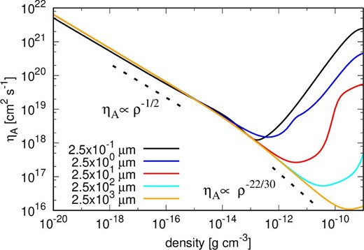
ηA as a function of density with the parameters of ModelA100Q25 in which we assume amin = 100 nm, q = 2.5, and ζCR = 10−17 s−1. The black, blue, red, cyan, and orange lines show the results of amax = 2.5 × 10⁻¹, 2.5 × 100, 2.5 × 101, 2.5 × 10², and |$2.5\times 10^{3}\, {\mu } {\rm m}$|, respectively.
Here, we assume that the temperature is given as T = 10[1 + γ(ρg|$/$|ρc)(γ − 1)] K, where γ = 5|$/$|3 and ρc = 4 × 10⁻¹³ g cm−3. The magnetic field is given as |$0.2 n_{\rm g}^{1/2}\, \mu \mathrm{G}$| (i.e., assuming flux freezing; see, e.g., Nakano et al. 2002). ζCR = 10−17s−1. With these assumptions of the temperature and magnetic field, and once the adsorption of charged particles by grains becomes negligible,ηA obeys
where the temperature dependence of C is included [equation (A18)].
We can see that ηA is well described by this power law at ρ < 10−11 g cm−3 (i.e., the simulated disk density region) once |$a_{\rm max} \gtrsim 250 \, {\mu } {\rm m}$|. Therefore, our assumption in appendix 1 seems justified when the dust size exceeds |$\gtrsim 100\, {\mu } {\rm m}$| (at least for ModelA100Q25). See Tsukamoto and Okuzumi (2022) for results with a wider variety of parameters.
