


Abstract
We built a Ka-band dual-circular-polarization low-noise receiver for the Misasa 54 m parabola antenna in Misasa, Japan. The antenna is designed to be combined with a transmitter and receiver system at the X band (around 8 GHz) and simultaneously with a receiver system at the Ka band. The Ka band is the frequency band around 30 GHz, which is important for deep-space communications and radio astronomy. The receiver comprises some waveguide components including a feed horn, a circular polarizer, and low-noise amplifiers. The components are installed in a vacuum vessel and are cooled to 4 K with a Gifford–McMahon refrigerator, providing low-noise performance. The receiver is capable of simultaneously handling the left- and right-hand circular-polarization (LHCP and RHCP) channels. The receiver-noise temperature was measured to be TRX ≃ 14 K in both the LHCP and RHCP channels. The system-noise temperature, including the antenna loss and atmospheric attenuation at the zenith, was measured to be Tsys = 36–37 K in both the LHCP and RHCP channels on a clear day in September at Misasa. When the receiver is used with the X-band transmitter, the system-noise temperature is maintained at Tsys ≃ 42 K in the RHCP channel. The degradation in the system-noise temperature is attributed to a frequency-selective reflector, which divides the signals in the X and Ka bands. There is no contamination from the transmitter to damage the receiver. The receiver has already been in use for deep-space communications and radio-astronomy observations. Our team in the radio-astronomy laboratory of ISAS/JAXA is responsible for the development of the receiver and the measurements of its performance.
1 Introduction
The Ka band used in deep-space telecommunications and radio astronomy is the frequency band around 30 GHz, where the atmospheric transmission loss is at a local minimum, located between the H2O absorption at 22 GHz and the O2 absorption at ∼60 GHz (e.g., figure 6.19 in Baars 2007). One advantage of this frequency band is that a wider bandwidth is available than with the X band, which is the frequency band around 8 GHz and which has been used in deep-space telecommunications. Thus, the Ka band promises to become an important band in the coming era of mass data transfer from deep-space explorers (e.g., Soriano et al. 2021).
At the same time, the Ka band is a popular observation band with the millimeter-wave Very Long Baseline Interferometer (mm VLBI), which is a powerful tool for geodesic and astrophysical studies of active galactic nuclei (e.g., Horiuchi et al. 2012; Charlot et al. 2020; Jacobs et al. 2021, 2022). In addition, some emission lines from interstellar molecules have been found in the frequency band, which include SO N, J = 0, 1–1,0 (ν = 30.00155 GHz), CH3OH 19(2,17)–19(1,18) (ν = 31.22671 GHz), and HC5N J = 12–11 (ν = 31.95178 GHz) (see NIST Recommended Rest Frequencies for Observed Interstellar Molecular Microwave Transitions).1 These lines are one of the key lines in radio astronomy, given that the SO lines are related to high-temperature chemistry in molecular clouds and that CH3OH molecules are enhanced by C-shock in molecular clouds (Hartquist et al. 1995). As such, the Ka band is an important band in radio astronomy (e.g., Soriano et al. 2021).
In response to demands in science and technology, the Ground Station for Deep Space Exploration and Telecommunication (GREAT) Project of the Institute of Space and Astronautical Science, Japan Aerospace Exploration Agency (ISAS/JAXA) constructed a millimeter-wave parabola antenna with a diameter of 54 m, called the Misasa 54 m antenna, in the vicinity of the Misasa summit of Yatsugatake mountains in Nagano, Japan (e.g., Toda et al. 2016; Toda & Asaki 2018; Oonishi et al. 2018). Figure 1a shows a photograph of the antenna. The antenna is meant to replace the Usuda 64 m antenna of the Usuda Deep Space Center (Hayashi et al. 1994). This antenna has been designed to be combined with a transmitter and receiver system in the X band and a receiver system in the Ka band, both of which are operated simultaneously. Figure 1b shows a schematic display of the beam-guide optics around the X-band transmitter and receiver system and the Ka-band receiver system. Incident signals in the X and Ka bands from the beam guide of the antenna are divided by a frequency-selective reflector (FSR) and sent to each feed horn. The transmitted signal from the X-band transmitter is reflected to the beam guide of the antenna by the FSR. The FSR is a Fabry–Pérot etalon operated in these frequency bands.
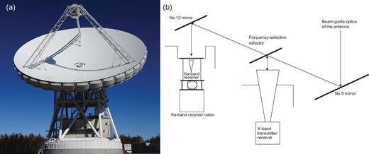
(a) Photograph of the Misasa 54 m antenna, built by ISAS/JAXA. (b) Schematic display of the beam-guide optics around the X-band transmitter and receiver and the Ka-band receiver of the antenna.
A core subsystem of the Ka-band receiver of the antenna comprises some waveguide (WG) components including a feed horn, a circular polarizer (WG-CP), and a low-noise amplifier (LNA). These components are installed in a vacuum vessel and are cooled to 4 K by a Gifford–McMahon (GM) refrigerator to suppress noise. Here we report the design and measured performance of the receiver, the development of which has been carried out by our team at the radio-astronomy laboratory of ISAS/JAXA. The detail of the antenna will be published separately (Y. Murata et al. in preparation). The nomenclature used in this paper accords with that of classical telecommunications technology.
2 Technical requirements for the Ka-band receiver of the Misasa 54 m antenna
2.1 Receiver-noise temperature
From the necessary conditions of telecommunication with deep-space explorers that will be launched by ISAS/JAXA, the sensitivity of the Ka-band receiver system of the Misasa 54 m antenna is required to be |$\frac{G}{T}\ge 59.33$| dB K−1 including atmospheric and rain attenuation at the antenna elevation of EL ≥ 15° (Toda et al. 2016; Toda & Asaki 2018; Oonishi et al. 2018). Here the term |$\frac{G}{T}$| shows a sensitivity in the classical telecommunications technology and is defined as |$\frac{G}{T}=G-10\log T_\mathrm{sys}$|, where G [dB] is the antenna gain and 10log Tsys [dB] is the system-noise temperature in the common logarithm. The required frequency range is the band from 31.8–32.2 GHz, which leads to the requirement that the receiver-noise temperature be TRX ≤ 35 K (Oonishi et al. 2018; Tabuchi et al. 2018). Ka-band receiver systems have been used in other classical antennas, including the Nobeyama 45 m telescope (e.g., Ukita & Tsuboi 1994). The receiver-noise temperature is degraded by the additional noise of the feed horn and WG vacuum flange at room temperature. Their feed horns should be placed at the cold stage in the receiver vessel to suppress noise, as they are too large to install in the receiver vessel. Thus, it has been difficult in conventional ways to satisfy the mentioned requirement for the receiver-noise temperature. However, recent developments in cryotechnology, especially the improvement in thermal insulation (e.g., Britcliffe et al. 2004; Choi et al. 2013), enable us to install the feed horn on the 4-K stage in the receiver vessel in our system. Although the tip of the feed horn cannot be cooled down to exactly 4.0 K due to thermal radiation from outside when the feed horn is placed on the 4-K stage, the additional noise should be dramatically decreased. If the transmission loss by the feed horn and WG vacuum flange is assumed to be the typical value of Lfh + wvf = 0.2 dB, the improvement in the receiver-noise temperature is ΔTRX ∼ 14 K when the feed horn is cooled. The way that the feed horn is placed on the 4-K stage is described in the following section.
2.2 Isolation between signals in the X and Ka bands
In our system, the Ka-band receiver is used simultaneously with the X-band transmitter (see the introduction). This simultaneous use has been realized in several methods in telecommunication antennas in the world (e.g., Stanton et al. 2001; Hoppe & Reilly 2004; Khayatian & Hoppe 2008; Soriano et al. 2021). In our case, we used an FSR to divide signals in the X and Ka bands—see the introduction and also Y. Murata et al. (in preparation). A requirement is that even when a signal with P = 40 kW (76 dBm) at ν = 7.2 GHz, which is the specification of the transmitter, is emitted from the X-band transmitter, the performance of the Ka-band receiver should not be degraded.
We conjecture that stray light reaches the vacuum beam window of the Ka-band receiver from the horn antenna of the X-band transmitter, attenuating by free-space propagation loss in the beam-guide optics. The loss is calculated to be at least ∼64 dB in the final design. Even when the stray light goes through the vacuum beam window of the Ka-band receiver to the feed horn, it never gets to the output WG of the WG-CP, which is located downstream of the feed horn for the following reasons (see figure 2). The output of the feed horn is a circular WG with a diameter of D = 7.3 mm, and the cutoff frequency of the lowest-order mode is calculated to be νcutoff = 24.08 GHz. The output WG of the WG-CP is a rectangular WG of WR-28 and the cutoff frequency of the lowest-order mode is calculated to be νcutoff = 21.08 GHz. These cutoff frequencies are much higher than ν = 7.2 GHz. However, although the fourth and higher harmonics can go through the cutoffs, the power levels of such higher-order harmonics leaking from the X-band transmitter should be much smaller than those of the signals at ν = 7.2 GHz and low-order harmonics. These harmonics are suppressed by a band-pass filter (BPF) placed on the 4-K stage. The details of the BPF are described in the following section.
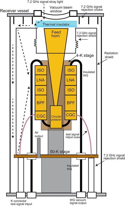
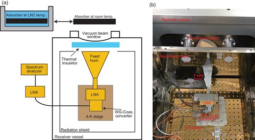
Schematic display of the circuit on the 4-K stage of the Ka-band receiver. The signal from the antenna optics is incident on the feed horn through the vacuum beam window and the thermal insulator. The signal travels through the feed horn to the circular polarizer (WG-CP). The signal travels through the BPF (figure 9a) to the cryogenic LNA, which has isolators (ISOs) at the input and output. The amplified signal by the LNA travels through the insulated WGs and WG vacuum-signal output to the outside of the receiver vessel. These components are well isolated by the 7.2 GHz signal-rejection shield and 7.2 GHz signal-rejection choke that are added to the radiation shield. The signal for several tests is injected by the cross-guide coupler (CGC) that is located before the BPF. In addition, the air in the radiation shield is exhausted through the air output on the 50 K stage when the receiver vessel is exhausted with a vacuum pump. The air output is a circular pipe, which has, as a circular WG, a cutoff frequency of a value much higher than 7.2 GHz. Broken line arrows show possible paths of 7.2 GHz signal stray light.
One of the possible paths is that the incident stray light in the radiation shield should be received by the power-supply cables and invade the high-electron-mobility transistor (HEMT) of the cryogenic LNA directly without passing through the tuning circuit (see the broken arrows in figure 2). The stray light travels through small openings of the radiation shield in the receiver vessel. The crosstalk by the incident stray light is expected to affect the LNA unless such openings are closed. On the other hand, the room-temperature electronics components including LNAs are located in the Ka-band receiver cabin, which is shielded from the 7.2 GHz signal. The permissible input level of the cryogenic LNA is estimated to be Pmax,in = P1 dB − GLNA = −38 dBm at 32 GHz, where GLNA is the gain of the cryogenic LNA (see subsection 4.4), from the P1-dB compression output level of the LNA, P1 dB = −10 dBm, which was available from the laboratory of the LNA maker. Although the permissible input level is for the signal at 32 GHz, this was used as the typical value because the signal at 7.2 GHz in this case is assumed to invade the HEMT directly. The isolation requirement or the ratio between the signal power level and permissible level is calculated to be Iso. ≥ 76 + 38 = 114 dB. Given the large level, even a small amount of stray light of a transmitted signal may have to be considered seriously. The isolation for the receiver vessel is required to be Iso. ≳ 114 − 64 = 50 dB after subtracting the attenuation by the free-space propagation loss. The way in which the stray light is suppressed in the receiver vessel and small openings are closed is described in the following section.
2.3 Ripple level for the frequency range
The ripple level shows the degree of flatness in the frequency range at the signal output. The performance of the AD conversion in the backend electronics depends on the level. The reflections at the ends of cables and WGs and/or transmission performance of components of the receiver like LNAs and band-pass filters can degrade the ripple level. The system requirement for the ripple level is 2 dB/100 MHz. We measured the ripple levels of the candidate components and assembled the receiver from only the selected components that have comparatively low ripple levels. Table 1 summarizes the system requirements and measured performance of the constructed receiver.
System requirements and evaluation results of the Ka-band receiver.
| Item | Requirement | Result |
|---|---|---|
| Frequency range | f = 31.8–32.3 GHz | Satisfied |
| Receiver-noise temperature | TRX ≤ 35 K | TRX ∼ 14 K |
| Receiver gain | GRX = 62 dB* | Satisfied |
| Reflection coefficient at the input | S11 ≤ −19.1 dB† | S22‡ ∼ −28 dB |
| Isolation between signals in X and Ka bands | Iso. ≥ 114 dB | Iso. ∼ 117 dB |
| (Isolation for the receiver vessel | Iso. ≥ 50 dB | Iso. = 53 ± 2 dB) |
| Ripple level in the frequency range | ΔP/ΔF ≤ 2 dB/100 MHz | ΔP/ΔF ∼ 0.2 dB/100 MHz |
| Vacuum beam window | No condensation in all weather conditions | Satisfied |
This was derived from the permissible input level of the following electronics, −15 dBm (Oonishi et al. 2018), the maximum possible input, −80 dBm, which is calculated by 10log kTB = 10log [k × 350 [K] × (2 × 10⁹ [Hz])], and the allowance of 3 dB (Tabuchi et al. 2018).
This is for the input of the feed horn, which was evaluated by the antenna team of the Mitsubishi Electric Company based on a physical optics simulation of the antenna. The reflection coefficients of the WG-CP, cross-guide coupler, BPF, and isolator had been measured to be S11 < −20 dB, S11 < −30 dB, S11 < −20 dB and S11 < −21 dB, respectively. These would not cause trouble. Only the value for the feed horn remained to be measured.
We measured the reflection coefficient at the output, S22, of the feed horn because S11 cannot be measured directly.
3 Structure of the Ka-band receiver
3.1 Circuit on the 4-K stage
Figure 2 shows a schematic display of the circuit on the 4-K stage of the Ka-band receiver. Figures 3a and 3b are photographs of the interior structure of the Ka-band receiver where the radiation shield is removed. The receiver is capable of using simultaneously the channels of the left- and right-hand circular polarizations (LHCP and RHCP). The feed horn, WG-CP, BPF, and cryogenic LNA are installed on the 4-K stage. The feed horn is a dual-mode conical horn antenna with a circular WG output, which is designed to match the beam-guide optics of the Misasa 54 m antenna designed by the Mitsubishi Electric Company and manufactured by Oshima Prototype Engineering. It is operated at a physical temperature of Tphysical = 4 K. The signal from the antenna optics is incident on the feed horn by way of the vacuum beam window and the thermal insulator. The signal travels from the feed horn to the WG-CP, where it is converted from the LHCP and RHCP signals in the circular WG input of the WG-CP to two linear polarization signals in the rectangular WG outputs of the WG-CP respectively. We designed the WG-CP to show optimum performance in the frequency range of the Ka band, and it has a four-stepped septum at the center of the input WG (e.g., Chen & Thandoulas 1973). The WG-CP was manufactured by Oshima Prototype Engineering and is operated at Tphysical = 4 K (see figure 9a below for the properties at room temperature). The signal output from the WG-CP travels to the cryogenic LNA by way of the BPF. The LNA is equipped with isolators (ISOs) at the input and output to improve S11 and S22. The cryogenic ISOs were purchased from QuinStar Technology, Inc. (model QKF-A). In the frequency range from ν = 31.8–32.3 GHz, the reflection coefficients, insertion losses, and isolations were measured to be S11 ≲ −21 dB, S21 ≲ 0.3 dB, and S12 ∼ −19 dB, respectively. The RHCP channel is mainly used for telecommunication. It is possible to remove the BPF of the LHCP channel from the system if required, such as for radio-astronomical uses. The amplified signal by the LNA then travels through the insulated WGs and WG vacuum-signal output to the outside of the receiver vessel. We injected the signal for tests by the cross-guide couplers (CGCs) that are located in front of the BPFs. The coupling values, reflection coefficients, and insertion losses were measured to be Coup. ∼ −30 dB, S11 ≲ −30 dB, and S21 < 0.1 dB, respectively. These components are well isolated by the 7.2 GHz signal-rejection shield and 7.2 GHz signal-rejection choke that are added to the radiation shield.
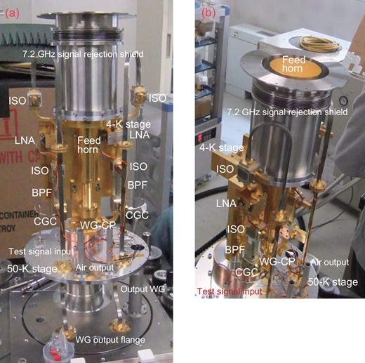
(a) Interior structure of the Ka-band receiver where the radiation shield is removed. (b) Another view of the interior structure of the Ka-band receiver from a different angle.
In addition, the air in the radiation shield on the 50-K stage is exhausted through the air output when the receiver vessel is pumped out with a vacuum pump (see figures 2 and 3). The air output is made of circular pipes, which are designed to have, as a circular WG, a cutoff frequency of a value much higher than 7.2 GHz (νcutoff = 20.68 GHz). Air in the radiation shield can be exhausted through the air output, but the 7.2 GHz signal and its second harmonics cannot spread into the radiation shield through it.
3.2 Circuits at room temperature
Figure 4 shows a photograph of the post-stage circuit including room-temperature LNAs of the Ka-band receiver. The circuit is installed on the outside of the receiver vessel. The output signal from the WG vacuum-signal output of the receiver vessel travels through the WG (WR-28) to the room-temperature LNAs. We purchased LNAs (model QLN-32022846-A) from QuinStar Technology, Inc. According to the catalog specification, the LNA noise temperature and gain are TLNA = 260 K and GLNA = 46 dB, respectively. The LNA is equipped with ISOs at the input and output to improve S11 and S22. The effective frequency range of the LNA is guaranteed to encompass 31–33 GHz in the specification. Since the components other than the LNA are effective for a wider frequency range than 31–33 GHz (e.g., the room-temperature ISO is effective from 30–37 GHz), replacing a room-temperature LNA of another frequency range and removing the BPF in the receiver vessel enables us to perform astronomical observations in the wider frequency range.
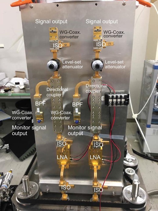
Post-stage circuit including room-temperature LNAs of the Ka-band receiver. The monitor output is branched by the directional coupler. The room-temperature LNA is replaceable.
The typical value of P1 dB of this LNA is P1 dB = +10 dBm at 32 GHz, which was available from the laboratory of the LNA maker. The permissible input level of the LNA is PIN = P1 dB − G = −36 dBm. On the other hand, the maximum input level of the cryo-LNA is −80 dBm, as mentioned previously (see the caption of table 1). The gain of the cryogenic LNA is 28 dB. The maximum input level of the LNA is −52 dBm, which is sufficiently small compared to the permissible input level. In addition, although the IP3 was not obtained from the maker, it would not cause trouble in this case because IP3 is usually several or 10 dB higher than P1 dB. These show that this amplifier operates in the linear region.
The composite gain of the cryogenic and room-temperature LNAs is ∼74 dB, which is much larger than the required gain of 62 dB for the input level of the backend electronics where the cable loss between the output of the receiver and the input of the backend electronics is fully taken into account. Thus, the signal amplified by the LNAs is adjusted to the input level of the backend electronics by the level-set attenuator. The monitor output of the amplified signal is branched by a directional coupler placed between the LNA and the level-set attenuator.
4 Measurements of the performance of the receiver components
4.1 Vacuum beam window and cryogenic feed horn
Figure 5a shows a schematic display of the vacuum beam window and thermal insulator. The vacuum beam window is made of a half-wavelength Teflon plate to maintain the vacuum and a 50-|$\mu $|m-thick Teflon sheet to prevent condensation of water vapor on the window. The window is circular with a diameter of D = 120 mm. The most common material for vacuum windows for this type of purpose is a thin Kapton sheet. However, the requirement of the reflection coefficient (return loss) at the input, S11, in the frequency range from ν = 31.8–32.3 GHz for telecommunication is as low as S11 = −19.1 dB, which corresponds to Voltage Standing Wave Ratio (VSWR) |$=1.25$|. It is difficult to construct windows from thin Kapton sheets that satisfy this degree of low reflection. Thus, we employed a half-wavelength-plate technique, in which the reflected lights of the incident and outgoing waves interfere and disappear. One problem is that the thickness of the half-wavelength Teflon plate cannot be determined from the published permittivity data of Teflon because its accuracy is not sufficient for this technique. Hence, we measured it with the following procedure. We prepared Teflon plates of differences in thickness of Δt = 0, ±0.1, and ±0.2 mm from the expected half-wavelength to determine the optimum thickness. Although, ideally, S11 should be measured, it cannot be measured directly. Hence, instead, we measured the reflection coefficient at the output, S22, of the feed horn in the case in which the vacuum beam window and the thermal insulator are installed in front of the feed horn. We searched for the thickness with which S22 is minimum at 32 GHz. Figure 5a shows a schematic display of the measurement set-up of S22 of the feed horn when the vacuum beam window and the thermal insulator are installed. In the measurement, we used a vector network analyzer (VNA), an Anritsu MS46322A-040. The VNA was calibrated with the one-port-calibration method using “Short,” “Open,” and “Load” calibrators. The calibration plane was at the output of the horn. Here, “Short” is a metal plate that closes the input of the circular–rectangular WG converter. “Open” is a metal plate with a half-wavelength shifter or a quarter-wavelength WG. “Load” is a non-reflective terminator. We used ECCOSORB CV-3 as the absorber, which was placed in front of the window. Note that we used the absorber in all the measurements presented in this paper, including the liquid-nitrogen-temperature load.
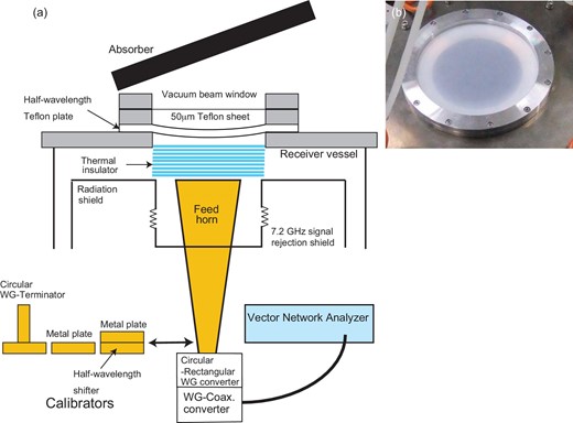
(a) Schematic display of the vacuum beam window and thermal insulator. The vacuum beam window is made of a half-wavelength Teflon plate and 50-|$\mu $|m-thick Teflon sheet. The thermal insulator is a stack of sheets of foamed polystyrene, which is placed between the vacuum beam window and the tip of the feed horn. This also shows the measurement set-up of S22 of the feed horn when the vacuum beam window and thermal insulator are installed. The vector network analyzer is an Anritsu MS46322A-040. (b) Outside view of the 50-|$\mu $|m-thick Teflon sheet of the vacuum beam window.
Figure 6a shows the measured values of S22 in the cases where the vacuum window of the Teflon plate of t = 3.3 mm and thermal insulator are/are not installed in front of the feed horn. Figure 6b shows an enlargement around 32 GHz. Figure 6c shows the measured values of S22 at t = 3.3 and 3.5 mm as examples to demonstrate our searches. The thickness difference of |Δt| = 0.2 mm corresponds to a pass-band frequency shift of 1.8 GHz. As a result, we measured S22 at t = 3.3 mm to be ∼ − 28 dB, which corresponds to |$\mathit {VSWR}\sim 1.08$|. It is also suitable that the center frequency of the pass band is located around 32 GHz. Then, the optimum thickness at 32 GHz was derived to be t = 3.3 mm. In addition, the additional noise at 32 GHz of the half-wavelength Teflon plate is expected to be ∼0.2 K (e.g., Britcliffe et al. 2004). The additional noise at 32 GHz of the thermal insulator is expected to be ∼1 K (e.g., Britcliffe et al. 2004).
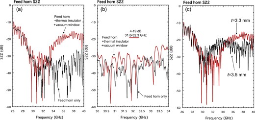
(a) Measured S22s in both the cases where only the feed horn is installed and the vacuum window and thermal insulator are installed in front of the feed horn. (b) Enlargement of panel (a). The specification of S22 is lower than −19 dB in the frequency range from ν = 31.8–32.3 GHz according to the telecommunication requirements. S22 is measured to be −28 dB even when the vacuum window and thermal insulator are used. (c) Measured S22s at t = 3.3 and 3.5 mm in the case where the vacuum window and thermal insulator are installed in front of the feed horn.
If the vacuum beam window is exposed to the air in the beam guide of the 54 m antenna, the vacuum beam window may attract condensation because the air is equivalent to the outside air. To prevent potential condensation of water vapor, the Teflon plate is covered with a Teflon sheet |$50\, \mu $|m in thickness and its outside is continuously aired during operation by a fan, which is placed at the outside of the window.
The thermal insulator is placed between the vacuum beam window and the tip of the feed horn (figure 5a). If there is no thermal insulator, the heat over 5 W is incident to the receiver vessel through the vacuum beam window. Since the cooling capacity of the GM refrigerator is 1.5 W at Tphysical = 4.2 K according to the catalog specification (Sumitomo Heavy Industry (SHI) RDK-415D), components in the receiver vessel cannot be cooled. It is necessary to use a high-quality thermal insulator. We used a stack of 10 thin foamed polystyrene sheets as the thermal insulator (Choi et al. 2013), which is almost transparent in the Ka band (e.g., Britcliffe et al. 2004) and optically thick in the infrared. According to Choi et al (2013), the physical temperature of the innermost sheet is expected to be Tphysical = 165 K. The analysis of the relation between incident heat and cooling capacity of the receiver is shown in figure 7. The incident heat to the 4-K stage through the vacuum beam window is expected to be suppressed to a value smaller than 0.5 W by the thermal insulator. In fact, this value is the worst-case scenario because the heat should be completely absorbed by the 4-K stage. Consequently, the total incident heats from the 300-K stage to the 50-K stage and from the 50-K stage to the 4-K stage are expected to be ∼10 W and ≲0.7 W, respectively, which are smaller than the cooling capacities of the refrigerator. We conducted a refrigerator test with the receiver vessel with all components assembled and found that the 4-K stage was cooled to a physical temperature of Tphysical = 3.6 K within 12 h. Then the physical temperature of the radiation shield was Tphysical = 44 K. This result proves that the thermal insulator works well.
![Analysis of the relation between the incident heat and cooling capacity of the Ka-band receiver. The incident heat from Tphysical = T1 K to Tphysical = T2 K, $\dot{Q}_{21}$, is calculated according to the following formulae: $\dot{Q}_{21}=\frac{A}{L}\int ^{T_1}_{T_2}\kappa (T)dT$ in the case of heat conduction, where A, L, and κ are the cross-section, length, and thermal conductivity of the conductor, respectively, and $\dot{Q}_{21}=A\sigma [\epsilon (1)T_1^4-\epsilon (2)T_2^4]$ in the case of thermal radiation, where σ and ε are the Stefan–Boltzmann constant and the emissivity of the surface, respectively. The GM refrigerator, which cools the receiver, is assumed to be a Sumitomo Heavy Industry (SHI) RDK-415D.](https://oup.silverchair-cdn.com/oup/backfile/Content_public/Journal/pasj/75/3/10.1093_pasj_psad020/2/m_psad020fig7.jpeg?Expires=1749408603&Signature=2DXPyM8PcI4jXJpHcq~wygy4vB6kBnwIpIEJNEcnddBm5gmq~ZdIikl91RE-Zjazj7TGkaxIhbLvhSrNklBIyWDMkjj3kBnL7ADJ8eYL-EFOH9U3oVYFyOLlqDVcjiSQmAS01UyHRT0EhjTmbMTZzAygJ5leXKcGzptClY8vRGGrDfAZjFMyMEVrhf8AuZKgvrDWvi6TDoFJBmlfa-K4M7yuGWnchJe198o9-jNHXHc~abD2wrFcxk1PQIwHwiwpG~inG1RjsTb6kfaHee2e2ULYaLENNPW-ezbyqYImvfwA1F0gwkP569kOpxRFQ6G4x8hGq~LqWzCYkRBm4SiWww__&Key-Pair-Id=APKAIE5G5CRDK6RD3PGA)
Analysis of the relation between the incident heat and cooling capacity of the Ka-band receiver. The incident heat from Tphysical = T1 K to Tphysical = T2 K, |$\dot{Q}_{21}$|, is calculated according to the following formulae: |$\dot{Q}_{21}=\frac{A}{L}\int ^{T_1}_{T_2}\kappa (T)dT$| in the case of heat conduction, where A, L, and κ are the cross-section, length, and thermal conductivity of the conductor, respectively, and |$\dot{Q}_{21}=A\sigma [\epsilon (1)T_1^4-\epsilon (2)T_2^4]$| in the case of thermal radiation, where σ and ε are the Stefan–Boltzmann constant and the emissivity of the surface, respectively. The GM refrigerator, which cools the receiver, is assumed to be a Sumitomo Heavy Industry (SHI) RDK-415D.
Small amounts of nitrogen gas, oxygen gas, water vapor, and other compounds in the air pass through the half-wavelength Teflon plate of the vacuum beam window and leak into the receiver vessel. They eventually condense on the 4-K stage and the radiation shield and freeze on them. This type of contamination continues during receiver operation. When refrigeration is stopped, they return to gas. If the volume at 1 atm (1 × 10⁵ Pa) of the released gas is much larger than the volume of the receiver vessel, the gas pressure may become high enough to break the vacuum beam window. In the vacuum test with the receiver vessel, the vessel was exhausted by a turbo molecular pump, ULVAC YTP50SA, to the criterion for the start of refrigerating, 5 Pa, within 30 min. The pressure reached 5 × 10⁻² Pa after over 10 h of exhausting. When the receiver vessel was left for 15 d after the pump stop, the pressure reached 1.3 × 10³ Pa. From this measurement, the leak speed is estimated to be ∼1.4 × 10⁻³ mol d−1. When refrigeration is stopped after a 1-yr operation, the pressure will increase up to ∼0.3 atm (∼3 × 10⁴ Pa). With this estimate, we conclude that the released gas would not break the vacuum beam window in and after nominal operations of the system.
4.2 Circular polarizer
Figure 8 shows a schematic display of the measurement set-up for the transmission loss and cross-polarization of the WG-CP using a vector network analyzer (VNA) at room temperature. We used an Anritsu MS46322A-040 as the VNA. The configuration in the figure is the RHCP–RHCP configuration, which measures the product of RHCP transmission losses of the WG-CPs (measured L). Alternatively, if the RHCP–LHCP configuration is adopted, the sum of RHCP cross-polarization is measured (measured Xpol). Note that with this measurement set-up, we can measure only the mean of the transmission loss and cross-polarization of two circular polarizers. The mean transmission loss and cross-polarization are derived from measured L and measured Xpol according to Ltrans [dB] |$= \frac{\mathrm{measured}\ L}{2}$| and Xpol [dB] = measured Xpol − 3 dB, respectively.
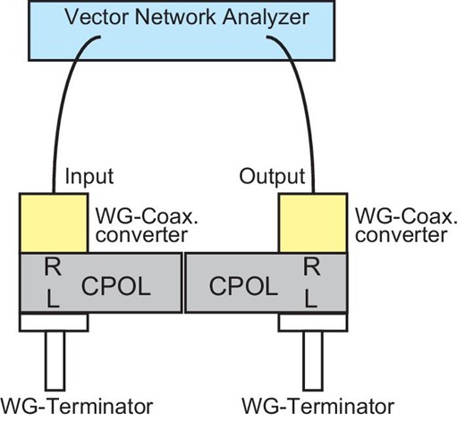
Schematic display of the measurement set-up of the circular polarizer at room temperature. This is the RHCP–RHCP configuration, which measures the product of RHCP transmission losses of the WG-CPs. In the case in which the RHCP–LHCP configuration is adopted, the sum of the RHCP cross-polarizations of the WG-CPs is measured. The vector network analyzer is an Anritsu MS46322A-040.
Figure 9a shows the mean transmission loss and cross-polarization for the frequency range from 31–33 GHz. The transmission loss in the RHCP channel appears to be ∼0.1 dB better than that in the LHCP channel. However, the difference may be attributed to calibration error. The cross-polarizations for them are similar in the range lower than an irregularity found at around 32.65 GHz. The irregularity may be caused by a misalignment of the centers of the polarizers in the measurement set-up. Even if the irregularity is real, it is not in the required frequency range. The transmission loss and cross-polarization in the frequency range are found to be Ltrans ∼ 0.2 dB and Xpol ∼ −40 dB, respectively, in both the LHCP and RHCP channels. In addition, the reflection coefficients at the input were also measured to be S11 < −20 dB in the frequency range.
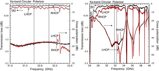
(a) Mean transmission loss and cross-polarization of LHCP and RHCP measured with the Ka-band circular polarizer at room temperature in the measurement set-up shown in figure 8. The parallel vertical lines indicate the frequency range from 31.8–32.3 GHz required for telecommunication. The transmission loss and cross-polarization are measured to be Ltrans ∼ 0.2 dB and Xpol ∼ −40 dB in both the LHCP and RHCP, respectively. (b) Mean transmission loss and cross-polarization of LHCP and RHCP in a wide frequency range of 26–40 GHz. The parallel vertical lines are the same as in panel (a). The obtained transmission loss is Ltrans < 0.2 dB in the frequency range of 27–37 GHz except for several dips.
Figure 9b shows the mean transmission loss and cross-polarization at room temperature in a wide frequency range of 26–40 GHz. The transmission loss is as low as Ltrans < 0.2 dB in a frequency range of 27–39 GHz, except for several irregularities. Like the discussion for the result presented in figure 9a, some of the irregularities may be artifacts originating in the imperfect measurement set-up. The wide-frequency characteristics demonstrate that our system shows good performance for radio-astronomy use. After the measurements, we installed them in the interior structure of the Ka-band receiver.
4.3 Band-pass filter and 7.2 GHz signal-rejection shield
The transmission loss, S21, and input reflection, S11, of the BPF were measured with the VNA, Anritsu MS46322A-040, at room temperature. Figures 10a and 10b show the obtained S11 and S21 of the filter, which is used in the RHCP channel. The obtained S21 and S11 were S21 ≲ 0.8 dB and S11 ≲ −20 dB in the frequency range of 31.8–32.3 GHz, respectively. The losses at the harmonic frequencies were found to be as large as L ≳ 65 dB. Then, the isolation including the free-space propagation loss is expected to be as large as L ≳ 129 dB, which is much larger than the requirement, L ∼ 114 dB (subsection 2.2).
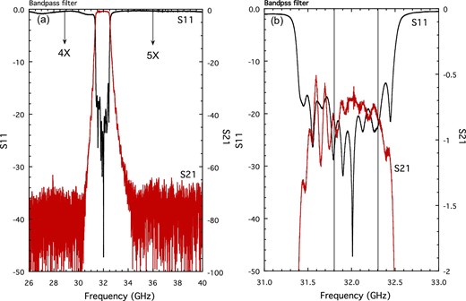
(a) Measured S11 and S21 of the RHCP band-pass filter at room temperature. The arrows indicate the (4X) fourth and (5X) fifth harmonics of the 7.2 GHz signal. (b) Enlargement of panel (a). The parallel vertical lines indicate the frequency range of 31.8–32.3 GHz required for telecommunication.
In order to suppress the incident stray light that comes through any openings of the radiation shield, the openings should be eliminated. In our initial model, relatively large openings were present around the feed horn and cables from the 50-K stage to the inside wall of the vessel. We closed the openings with thin stainless steel pipe structures (figures 2 and 3). In addition, we placed the choke structure to reject the 7.2 GHz signal propagating along the inside wall of the receiver vessel on the inside wall (figure 2).
The isolation by these structures was measured in the following set-up (see also figures 11a and 11b). The small ground plane antenna was placed near the LNA power-supply cables in the radiation shield as a nearly omni-directional probe antenna (see figure 21-10 in Kraus & Marhefka 2003), and the horn antenna was placed on the outside of the receiver vessel as the transmitter at 32 GHz. First, we measured the signal level at 32 GHz received by the probe antenna, using an Anritsu MS2725C spectrum analyzer, where the receiver vessel and radiation shield were removed (see figure 11a). This signal level was used as the reference level. Next, we did the same but with the radiation shield and 7.2 GHz signal-rejection shield installed (see figure 11b), and found that the signal level was weakened from the reference level, presumably due to the isolation effect. The isolation due to these structures was derived as 53 ± 2 dB.
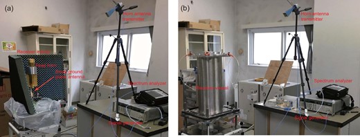
(a) Snapshot of the isolation measurement of the Ka-band receiver in the set-up where the receiver vessel, radiation shield, and 7.2 GHz signal-rejection shield were removed. The small ground plane antenna is placed near the LNA power-supply cable in the radiation shield (indicated by a red arrow) as a nearly omni-directional probe antenna, and the horn antenna is placed on the outside of the receiver vessel as the transmitter. (b) Snapshot of the isolation measurement of the Ka-band receiver in the set-up where the receiver vessel, radiation shield, and 7.2 GHz signal-rejection shield are properly installed.
The isolation including the free-space propagation loss is estimated to be L ∼ 53 + 64 = 117 dB, which is larger than the requirement, L ∼ 114 dB (subsection 2.2). We should note, however, that the requirement was derived on the basis that all the stray light received by the power-supply cables was transferred to the input of the LNA. In reality, the stray light received by the power-supply cables reaches the LNA through a feed-through capacitor, which is known to have a large insertion loss in microwaves. Consequently, the estimated isolation is sufficient in realistic cases for suppressing the degradation in the receiver.
4.4 Cryogenic low-noise amplifier
The receiver-noise temperature was estimated using the following equation:
where Lvc+ti and Tvc+ti are the combined loss and additional noise of the vacuum beam window and thermal insulator at room temperature, respectively. From published data (e.g., Britcliffe et al. 2004), they are supposed to be Lvc+ti = 0.996 or −0.018 dB and |$T_\mathrm{vc+ti}=293(\frac{1}{L_\mathrm{vc+ti}}-1)=1.2$| K, respectively. In fact, the thermal insulator should have a temperature gradient distributed from room temperature to the temperature of the radiation shield. Given that, the above-quoted additional noise should be the worst-case-scenario value. From the specifications of the catalogs, the loss and additional noise of the feed horn, WG-CP, CGC, ISO, and WG at Tphysical = 10 K are Lfh + WG-CP + CGC = 0.68 or −1.7 dB and |$T_\mathrm{fh+WG-CP+CGC+ISO+WG}=10(\frac{1}{L_\mathrm{fh+WG-CP+CGC}}-1)=5$| K, respectively. Then, the LNA noise temperature at Tphysical = 4 K was required to be TLNA,4 K = 20 K for TRX = 35 K.
Owing to good advancement in the development of InP high-electron-mobility transistor monolithic microwave integrated circuits (InP-HEMT MMICs) in the last two decades (e.g., Pospieszalski & Wollack 1997; Pospieszalski 2012), a cryogenic LNA with a noise temperature lower than TLNA < 20 K is now commercially available. We purchased two LNAs (model LNF-LNC23 42WB) from the Low Noise Factory (LNF), the LNA noise temperature of which is TLNA ≲ 8 K at Tphysical = 5 K in the frequency range of 24–35 GHz according to the catalog specification. We conducted a simple acceptance test for the LNAs, shown in figures 12a and 12b, in which we measured the LNA noise temperatures using the difference between the output powers where the input of the feed horn is terminated alternately by room-temperature and liquid-nitrogen-temperature loads. We also derived the gain of the LNA, using the difference between the output power at room-temperature load and the power of the blackbody. The acceptance test is only to check that the noise temperature of the LNA is better than the requirement shown in the previous paragraph.
(a) Schematic display of the LNA noise temperature measurement set-up as the LNA acceptance test. (b) Interior structure of the measurement set-up when the radiation shield is removed.
In the test, we used a Keysight N9030A spectrum analyzer to measure the output power levels. As a result, the LNA noise temperature and gain of one of the purchased LNAs at Tphysical = 4 K were obtained to be TLNA, 4 K = 8.5 ± 1.0 K and GLNA = 28 ± 0.3 dB, respectively, after the contributions of vacuum-signal window, liquid-nitrogen-temperature-load window, post-stage circuit at room temperature, and feed-horn spill-over were corrected. These were consistent with the catalog specifications. On the other hand, the parameters of the other LNA were measured to be TLNA, 4 K = 14.8 ± 1.0 K and GLNA = 28 ± 0.3 dB, respectively. Although the gain was consistent with the catalog specification, the LNA noise temperature was slightly higher than consistent with the catalog specification.
Water vapor in the laboratory often degrades apparently the measured LNA noise temperature through condensation on the liquid-nitrogen-temperature-load window, which is especially significant in the case of the measurement of an LNA with a temperature of TLNA ≲ 10 K. In the acceptance test, we covered the window with a thin film to prevent condensation (see the Appendix). Although the duration of time that the window was kept dry was moderately extended, the condensation was not prevented completely and the measurement noise temperatures consequently changed day to day. However, since the acceptance test at least proved that the LNA noise temperatures of LNAs are reasonably small, TLNA,4 K < 20 K, we proceeded and installed the cryogenic LNAs in the interior structure of the Ka-band receiver.
5 Measurements of the performance of the Ka-band receiver
5.1 Receiver-noise temperature in the laboratory
In the radio-astronomy laboratory of ISAS/JAXA, we measured the receiver-noise temperature of the Ka-band receiver, TRX, after installing all components in the circuit on the 4-K stage and post-stage circuit. Figures 13a and 13b show PR and PLN2 of the RHCP and LHCP channels, respectively, where PR is the output power when the input of the receiver is terminated by the absorber at room temperature TR, which was measured to be TR = 303 K, and PLN2 is the output power when the input of the receiver is terminated by the absorber at the liquid-nitrogen temperature, which is assumed to be TLN2 = 78 K. We used an Agilent E4446A spectrum analyzer to measure the output power levels. The ripple requirement is 2 dB/100 MHz in the frequency range of 31.8–32.3 GHz. The observed ripple was as small as 0.2 dB/100 MHz.
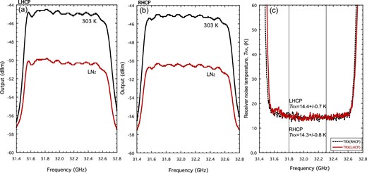
(a) Measured PR and PLN2 of the RHCP channel, where PR is the output power when the input of the receiver is terminated by the absorber at room temperature TR, which was measured to be TR = 303 K, and PLN2 is the output power when the input of the receiver is terminated by the absorber at the liquid-nitrogen temperature, which is assumed to be TLN2 = 78 K. (b) PR and PLN2 of the LHCP channel. (c) TRX of the RHCP and LHCP channels. TRX was derived with the hot–cold method.
The noise temperature TRX was then derived from the ratio |$\frac{P_\mathrm{ R}}{P_\mathrm{ LN2}}$| using the hot–cold method with the following formula:
Figure 13c shows the obtained TRX of the RHCP and LHCP channels. In the frequency range from 31.8–32.3 GHz, the TRX values of the RHCP and LHCP channels were measured to be TRX,LHCP = 14.3 ± 0.8 K and TRX,RHCP = 14.4 ± 0.7 K, respectively. These values are much better than the requirement for the receiver-noise temperature, TRX = 35 K. The additional noise by all the components including the feed horn is suppressed to ΔTRX ∼ 6 K. This result is consistent with the expected value of ΔTRX = 1.2 + 5 = 6.2 K shown in the previous section. According to Observing With The Green Bank Telescope 2021,2 the receiver-noise temperature of the Ka-band receiver of the Green Bank Telescope (GBT) is TRX = 20 K. The noise temperature TRX of our Ka-band receiver is as low as or lower than that of the GBT.
5.2 System-noise temperature at the Misasa 54 m parabola antenna
The Ka-band receiver was installed in the Ka-band receiver cabin of the Misasa 54 m antenna on 2019 September 6. After helium pipes had been connected from the cold head of the refrigerator to the compressor and coaxial cables had been connected from the post-stage circuit to the backend electronics, the receiver vessel was exhausted to <5 Pa with the turbo molecular pump and the receiver started to be refrigerated. The 4-K stage was cooled to a physical temperature of <3 K within 8 h.
The system-noise temperature, Tsys, was derived with the R–sky method from |$\frac{P_\mathrm{R}}{P_\mathrm{sky}}$| obtained on 2019 September 25, where we used a Keysight N9030A spectrum analyzer to measure the output power levels. Here, PR is the same as in the previous subsection but with a different room temperature of TR = 288 K, and Psky is the output power when the input is connected to the sky through the beam-guide optics. The weather was clear during the measurement. Figure 14a shows the obtained PR and Psky with and without the FSR of the RHCP channel. The ripple levels of the RHCP and LHCP channels are apparently larger than those measured in the laboratory (see figure 13). However, the larger ripple levels are probably caused by the branching cable used in the measurement because the degradations in the frequency characteristics resemble each other in the frequency range (see figures 14 and 15). The noise temperature Tsys is calculated using the following formula (see also Otoshi 2008) from the measured power ratio |$\frac{P_\mathrm{ R}}{P_\mathrm{sky}}$|:
Figure 14b shows the calculated Tsys for the system set-ups with and without the FSR of the RHCP channel. They were as low as Tsys = 42.4 ± 1.5 K and Tsys = 36.2 ± 0.8 K, respectively, at EL = 90° in the frequency range of 31.8–32.3 GHz. The degradation due to the FSR, ΔTsys ∼ 6 K, corresponds to the transmission loss in the FSR, L ∼ 0.086 dB, which must be mainly caused by ohmic loss on the reflector surface.
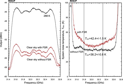
(a) Measured PR (in black) and Psky (in red) with and without the FSR of the RHCP channel. Here, PR is the output power when the input of the receiver is terminated by the absorber at a room temperature of TR = 288 K and Psky is the output power when the input is connected to the sky through the beam-guide optics. The weather was clear during the measurement. (b) Tsys at EL = 90° with and without the FSR of the RHCP channel, derived with the R–sky method.
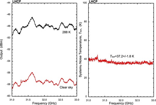
Same as figure 14 but for the LHCP channel and without the FSR only for Psky.
For use in radio-astronomy observations, the BPF of the LHCP channel at the 4-K stage is preferably removed before the Ka-band receiver is installed in the receiver cabin. The removal of the BPF widens the frequency range to 31–33 GHz. Figure 15a shows the PR and Psky of the LHCP channel. The observed ripple is 2 dB over the frequency range. The obtained Tsys was Tsys = 37.2 ± 1.8 K at EL = 90° in the frequency range of 31–33 GHz, where the weather was also clear. Figure 15b shows the obtained Tsys.
Our Ka-band receiver has already been used for deep-space communications and astronomical observations, including Japan–Australia observations in the X/Ka VLBI (e.g., Jacobs et al. 2021, 2022). The system-noise temperatures Tsys of both the RHCP and LHCP depend on the weather conditions. In clear-sky nights in winter, Tsys was measured to decrease to Tsys ∼ 29 K at EL = 90°. The system-noise temperature in the Ka band of the GBT is Tsys = 30–35 K (Observing With The Green Bank Telescope 2021; see footnote 2) and Tsys with our Ka-band receiver is similarly low or even lower. The sensitivity of the Misasa 54 m antenna reaches |$\frac{G}{T}\ge 66.9$| dB K−1 at EL = 80°. This means that the usable bit rate is four times better than the requirement in good weather conditions. Commissioning and verification of the whole system will be published separately (Y. Murata et al. in preparation).
Acknowledgements
We would like to acknowledge the excellent work of the Mitsubishi Electric Company and Oshima Prototype Engineering in designing and constructing the Misasa 54 m antenna and designing and manufacturing the Ka-band receiver components, respectively. We thank Mr Kenji Numata at ISAS for his continuous encouragement as the project manager of the GREAT project. We also thank Dr Kenta Uehara at the University of Tokyo and Dr Satomi Nakahara at the Graduate University for Advanced Studies (SOKENDAI) for extensive help during the laboratory measurements of the cryogenic LNAs.
Appendix. Liquid-nitrogen-temperature load
Figure 16 shows a schematic display of the liquid-nitrogen-temperature load, which is used in the measurements presented in this paper. The absorber sinks into the vessel filled with liquid nitrogen, which maintains the physical temperature of the absorber equal to that of the liquid nitrogen. The absorber is ECCOSORB CV-3. The wall of the vessel is made of foamed polystyrene, which works as a thermal insulator to hold liquid nitrogen. The foamed polystyrene wall is transparent to microwaves as long as water vapor does not condense on the surface. A thin polyvinylidene-chloride film (Saran Wrap, |$t\sim 10\, \mu $|m thick) is placed, though not physically touching, over the wall facing the feed horn. The thin film is also transparent to microwaves as long as water vapor does not condense on the surface. The wall has many micro-sized holes. Liquid nitrogen soaks into the wall and vaporizes in it. The nitrogen gas jets out of both sides of the wall. The ejected gas accumulates in the cavity between the thin film and the wall. Since the gas is very dry, it prevents water vapor from condensing on the outer surface of the wall. The cavity also prevents heat conduction from the thin film to the outer surface of the wall. In consequence, it is kept to prevent water vapor from condensing on the outer surface of the film for several ten minutes.
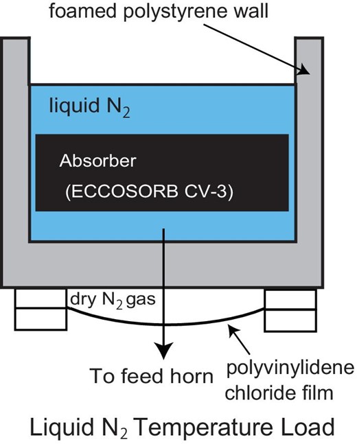
Schematic display of the liquid-nitrogen-temperature load.
