


Abstract
A novel collisionless shock jump condition is suggested by modeling the entropy production at the shock transition region. We also calculate downstream developments of the atomic ionization balance and the ion temperature relaxation in supernova remnants (SNRs). The injection process and subsequent acceleration of cosmic rays (CRs) in the SNR shocks are closely related to the formation process of the collisionless shocks. The formation of the shock is caused by wave–particle interactions. Since the wave–particle interactions result in energy exchanges between electromagnetic fields and charged particles, the randomization of particles associated with the shock transition may occur at a rate given by the scalar product of the electric field and current. We find that order-of-magnitude estimates of the randomization with reasonable strength of the electromagnetic fields in the SNR constrain the amount of CR nuclei and the ion temperatures. The constrained amount of CR nuclei can be sufficient to explain the Galactic CRs. The ion temperature becomes significantly lower than that in the case without CRs. To distinguish the case without CRs, we perform synthetic observations of atomic line emissions from the downstream region of the SNR RCW 86. Future observations by XRISM and Athena can distinguish whether the SNR shock accelerates the CRs or not from the ion temperatures.
1 Introduction
Collisionless shocks of supernova remnants (SNRs) are invoked as the primary sources of Galactic cosmic rays (CRs); however, the production process of CRs is an unsettled issue despite numerous studies reported. The most generally accepted and widely studied mechanism for CR acceleration is diffusive shock acceleration (Blandford & Ostriker 1978; DSA, Bell 1978). In the DSA mechanism, we assume energetic particles around the shock; the particles bounce back and forth between the upstream and downstream regions by scattering particles. The particle scattering results from interactions between plasma waves and the particles. The maximum energy of the accelerated particles depends on the magnetic-field strength and turbulence (e.g., Lagage & Cesarsky 1983a, 1983b). To explain the energy spectrum of the CR nuclei observed around the Earth, the maximum energy of the accelerated protons should be at least 1015.5 eV (the so-called knee energy). The knee energy can be achieved in the DSA mechanism by a magnetic-field strength of ≳|$100\,\, {\mu \rm {G}}$|, which is larger than the typical strength of ∼|$1\,\, {\mu \rm {G}}$| seen in the interstellar medium (ISM, Myers 1978; Beck 2001). Bell (2004) pointed out that the upstream magnetic field is amplified by the effects of a back reaction from the accelerated protons themselves. This amplification is called the Bell instability, whose growth rate is proportional to the CR energy density. Observations of nonthermal X-ray emissions around the SNR shocks imply the existence of amplified magnetic fields in the downstream region (e.g., Vink & Laming 2003; Bamba et al. 2005; Uchiyama et al. 2007). Hence, in a modern scenario of CR acceleration, the SNR shock is assumed to inject a considerably large amount of CRs (≳10% of the shock kinetic energy), and their effects on the background plasma are regarded as one of the most important issues. Since the wave–particle interactions also cause the formation of the collisionless shock, the injection of energetic particles, subsequent acceleration by the DSA mechanism, and the amplification of the magnetic field are closely related to the formation process. Although many kinetic simulations studying collisionless shock physics have been reported (e.g., Ohira 2013, 2016a, 2016b; Matsumoto et al. 2017; Caprioli et al. 2020; Marcowith et al. 2020), self-consistent treatment of the collisionless shock, including these effects, is currently incomplete due to the limitation of too-short simulation times compared to actual SNR shocks.
When the SNR shock consumes its kinetic energy to accelerate energetic, nonthermal particles, the downstream thermal energy can be lower than the case of adiabatic shock without CRs (e.g., Hughes et al. 2000; Helder et al. 2009; Morlino et al. 2013a, 2013b, 2014; Hovey et al. 2015, 2018; Shimoda et al. 2015, 2018b). Thus, we observe small downstream ion temperatures if the SNR shocks efficiently accelerate the CR nuclei (protons and heavier ions). In the near future, spatially resolved high-energy-resolution spectroscopy of the SNR shock regions will be achieved by the micro-calorimeter array with Resolve (Ishisaki et al. 2018) onboard XRISM (Tashiro et al. 2020) and with the X-IFU onboard Athena (Barret et al. 2018) providing precise line diagnostics of plasmas to represent the effect of the CR acceleration. Note that observations of γ-ray emissions possibly provide the amount of CR protons from the luminosities. However, it may be challenging to determine the amounts of CR nuclei individually. Thus, in this paper, we study the shock jump conditions of ions, including the effects of CR acceleration. To distinguish the case without CRs by future X-ray spectroscopy, we calculate the temporal evolutions of the downstream ionization structure and downstream ion temperatures resulting from the Coulomb interactions. From the calculations of the downstream values, we also perform synthetic observations of atomic lines, including the effects of downstream turbulence. Since the turbulence affects the line width by the Doppler effect, it is non-trivial whether the observed line width reflects the intrinsic ion temperature.
A typical example of the missing thermal energy measurement was provided by the SNR RCW 86 (Helder et al. 2009). RCW 86 is considered as the remnant of SN 185 (Vink et al. 2006), so its age is ∼2000 yr. The current radius is ∼15 pc, and the shock velocity is ∼3000 km s−1 with an assumed distance of 2.5 kpc (Yamaguchi et al. 2016), where we estimate the angular size as ∼40″. Since 2000 yr × 3000 km s−1 ≃ 6 pc < 15 pc, the blast wave has already decelerated. The mean expansion speed should be ∼109 cm s−1 if the radius becomes ∼10 pc within a time of ∼1 kyr. Such high expansion speed can be maintained for 1 kyr if the progenitor star explodes in a wind-blown cavity created by the progenitor system. Broersen et al. (2014) studied this scenario by comparing the X-ray observations and hydrodynamical simulations. They concluded that the progenitor star of SN 185 exploded as a Type-Ia supernova inside the wind cavity. The progenitor system could be a binary system consisting of a white dwarf and a donor star. In the present day, RCW 86 shows Hα filaments everywhere (Helder et al. 2013). The Hα emission means that the shock is now propagating into a partially ionized medium (Chevalier et al. 1980). In the case of a stellar wind from a massive star, the ionization front precedes the front of the swept-up matter (e.g., Arthur et al. 2011). Thus, the forward shock of RCW 86 may currently propagate in the medium not swept up by the wind. In this paper, we suppose such a scenario for RCW 86 and perform synthetic observations of the X-ray atomic lines.
This paper is organized as follows: In section 2, we review a physical model of the temporal evolutions of the downstream ionization balance and the ion internal energies. The ion temperatures are derived from the equation of state. Section 3 provides shock jump conditions as initial conditions for the downstream temporal evolution. We introduce shock jump conditions usually supposed in SNRs and a novel condition given by modeling the entropy productions of the ions due to the wave–particle interactions. The latter includes the effects of the CR acceleration, magnetic-field amplification, and ion heating balance. The results of the downstream temporal evolutions are summarized in section 4. In section 5, we perform synthetic observations of atomic lines, including the effects of the downstream turbulence. Finally, we summarize our results and future prospects.
2 Physical model of the downstream ionization balance and ion internal energies
Literature on the recombition rate.
| Ion | Literature | Ion | Literature | Ion | Literature |
|---|---|---|---|---|---|
| C+1 | Nahar and Pradhan (1999) | Mg+5 | Arnaud and Rothenflug (1985) | S+12 | Mewe, Schrijver, and Sylwester (1980a, 1980b) |
| C+2 | Nahar and Pradhan (1999) | Mg+6 | Zatsarinny et al. (2004) | S+13 | Mewe, Schrijver, and Sylwester (1980a, 1980b) |
| C+3 | Nahar and Pradhan (1997) | Mg+7 | Nahar (1995) | S+14 | Arnaud and Rothenflug (1985) |
| C+4 | Nahar and Pradhan (1997) | Mg+8 | Arnaud and Rothenflug (1985) | S+15 | Arnaud and Rothenflug (1985) |
| C+5 | Nahar and Pradhan (1997) | Mg+9 | Arnaud and Rothenflug (1985) | Fe+1 | Nahar and Pradhan (1997) |
| N+1 | Zatsarinny et al. (2004) | Mg+10 | Arnaud and Rothenflug (1985) | Fe+2 | Nahar and Pradhan (1997) |
| N+2 | Nahar and Pradhan (1997) | Mg+11 | Arnaud and Rothenflug (1985) | Fe+3 | Nahar and Pradhan (1997) |
| N+3 | Nahar and Pradhan (1997) | Si+1 | Nahar (2000) | Fe+4 | Nahar (1998) |
| N+4 | Nahar and Pradhan (1997) | Si+2 | Altun et al. (2007) | Fe+5 | Nahar and Pradhan (1999) |
| N+5 | Nahar (2006) | Si+3 | Mewe, Schrijver, and Sylwester (1980a, 1980b) | Fe+6 | Arnaud and Rothenflug (1985) |
| N+6 | Nahar (2006) | Si+4 | Zatsarinny et al. (2003) | Fe+7 | Nahar (2000) |
| O+1 | Nahar (1998) | Si+5 | Zatsarinny et al. (2006)* | Fe+8 | Arnaud and Rothenflug (1985) |
| O+2 | Zatsarinny et al. (2004) | Si+6 | Zatsarinny et al. (2003) | Fe+9 | Arnaud and Rothenflug (1985) |
| O+3 | Nahar (1998) | Si+7 | Mitnik and Badnell (2004)* | Fe+10 | Lestinsky et al. (2009)* |
| O+4 | Nahar (1998) | Si+8 | Zatsarinny et al. (2004) | Fe+11 | Novotný et al. (2012)* |
| O+5 | Nahar (1998) | Si+9 | Nahar (1995) | Fe+12 | Hahn et al. (2014)* |
| O+6 | Nahar (1998) | Si+10 | Arnaud and Rothenflug (1985) | Fe+13 | Arnaud and Rothenflug (1985) |
| O+7 | Nahar (1998) | Si+11 | Arnaud and Rothenflug (1985) | Fe+14 | Altun et al. (2007)* |
| Ne+1 | Arnaud and Rothenflug (1985) | Si+12 | Arnaud and Rothenflug (1985) | Fe+15 | Murakami et al. (2006)* |
| Ne+2 | Zatsarinny et al. (2003) | Si+13 | Arnaud and Rothenflug (1985) | Fe+16 | Zatsarinny et al. (2004) |
| Ne+3 | Mitnik and Badnell (2004)* | S+1 | Mewe, Schrijver, and Sylwester (1980a, 1980b) | Fe+17 | Arnaud and Rothenflug (1985) |
| Ne+4 | Zatsarinny et al. (2004) | S+2 | Nahar (1995) | Fe+18 | Zatsarinny et al. (2003) |
| Ne+5 | Nahar (1995) | S+3 | Nahar (2000) | Fe+19 | Savin et al. (2002)* |
| Ne+6 | Arnaud and Rothenflug (1985) | S+4 | Altun et al. (2007) | Fe+20 | Zatsarinny et al. (2004) |
| Ne+7 | Arnaud and Rothenflug (1985) | S+5 | Arnaud and Rothenflug (1985) | Fe+21 | Arnaud and Rothenflug (1985) |
| Ne+8 | Nahar (2006) | S+6 | Zatsarinny et al. (2004) | Fe+22 | Arnaud and Rothenflug (1985) |
| Ne+9 | Nahar (2006) | S+7 | Zatsarinny et al. (2006)* | Fe+23 | Mewe, Schrijver, and Sylwester (1980a, 1980b) |
| Mg+1 | Mewe, Schrijver, and Sylwester (1980a, 1980b) | S+8 | Zatsarinny et al. (2003) | Fe+24 | Nahar, Pradhan, and Zhang (2001) |
| Mg+2 | Zatsarinny et al. (2004) | S+9 | Mitnik and Badnell (2004)* | Fe+25 | Nahar, Pradhan, and Zhang (2001) |
| Mg+3 | Arnaud and Rothenflug (1985) | S+10 | Zatsarinny et al. (2004) | ||
| Mg+4 | Zatsarinny et al. (2004) | S+11 | Nahar (1995) |
3 Shock jump conditions
Here we give the initial conditions for the temporal developments of the downstream ionization balance and temperature relaxation by considering shock jump conditions. We introduce the conditions usually supposed in the SNR shocks from analogs of collisional shocks and the novel condition given by modeling the energy exchange between electromagnetic fields and particles.
3.1 Collisional shock model (Models 0, 1, and 2)
3.2 Collisionless shock model (Models 3, 4, and 5)
Here we consider another way of giving a shock transition with the CR acceleration. We assume that part of the shock kinetic energy is consumed for the generation of CRs and amplification of the magnetic field. The generated magnetic field is assumed to be disturbed (not an ordered field). In this model, we consider the randomization of the particles incoming from the far-upstream region at the shock transition region. The randomization is quantified by the entropy. We notice that the “randomization” results in a more isotropic particle distribution downstream than the pre-shock one (measured in the shock rest frame). In the collisional shocks, this may be called “thermalization;” however, the particle distribution may deviate from the Maxwellian in the collisionless shocks. We use “randomization” for both collisional and collisionless shocks in the following.
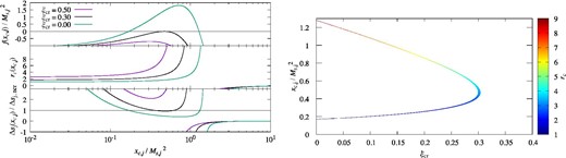
Left: Function of f = f(xc, j) defined in equation (47) (upper part), the compression ratio rc = rc(xc, j) (middle part), and Δsj(xc, j)/Δsj, ncr (lower part) for the proton with γ = 5/3. We set the parameters as ξcr = 0.5 (purple line), ξcr = 0.3 (black line), and ξcr = 0 (green line) with fixed values of v0 = 4000 km s−1, T0 = 3 × 10⁴ K, and |$1/\sqrt{\xi }_{\rm B}=v_0/(\delta B/\sqrt{4\pi \rho _0})=3$|. Note that |${\cal M}_{{\rm s},j}=197$|. Right: Solutions of f = 0 with fixed |$1/\sqrt{\xi }_{\rm B}=3$| and |${\cal M}_{{\rm s},j}=197$| for the proton. The horizontal axis shows the CR fraction ξcr and the vertical axis shows the pressure jump |$x_{{\rm c},j}/{\cal M}_{{\rm s},j}{}^2$|. The color indicates the compression ratio rc.
When ξcr becomes large, the two solutions approach each other, coinciding at ξcr ≃ 0.3 (multiple roots) and, finally, the solution vanishes. The multiple roots (ξcr = 0.3) give |$\tilde{v}^{\prime }_{\rm R}/v_0^{\prime }\simeq 0.7$| and Δsj/Δsj, ncr ≃ 0.93. Thus, the multiple roots may represent the shock transition giving the maximum Pcr feasible in our shock model. In this article, we set the maximum ξcr to compare the no-CR cases with the case of extremely efficient CR acceleration. The maximum ξcr is derived from the multiple roots of f = 0 with a given ξB.
For the case of v0 = 4000 km s−1 and T0 = 3 × 10⁴ K with given |$1/\sqrt{\xi _{\rm B}}=3$|, we obtain the maximum acceptable CR production ξcr ≃ 0.3, Δsj/Δsj, ncr ≃ 0.92–0.95 depending on mj, rc ≃ 3.29, and kTp, 2 ≃ 14.4 keV. Note that in the case of Model 0 (the usual collisional shock case), we obtain rc = 4.00 and kTp, 2 = 31.3 keV. The fraction of CRs ξcr = 0.3 seems to be reasonable for the SNR shocks as sources of Galactic CRs. From the subtraction of the energy fluxes of the thermal particles at the far upstream and downstream, we can regard that roughly 50% of the upstream energy flux is transferred to the nonthermal components. The fraction of magnetic pressure |$1/\sqrt{\xi _{\rm B}}=3$| corresponds to a magnetic-field strength of |$\delta B\simeq 611\,\, {\mu \rm {G}} ( v_0 /4000\,\, {\rm km\,\, s^{-1}} ) ( n_{\rm p,0}/1\,\, {\rm cm^{-3}})^{1/2}$|, which is consistent with the estimated strength from X-ray observations of young SNRs (e.g., Vink & Laming 2003; Bamba et al. 2005; Uchiyama et al. 2007). Thus, our parameter choice of |$1/\sqrt{\xi _{\rm B}}=3$| can be reasonable to adopt our model to the young SNR shocks.
Here we consider the choice of the maximum ξcr. In the case of collisional shock formed by hard-sphere collisions, for example, the collisions result in one of the most efficient randomizations of particles. Thus, the collisional shock can “easily” dissipate its kinetic energy within the mean collision time. In the collisionless plasma, such an efficient randomization process is absent. The particles in the plasma tend to behave as “nonthermal” particles resulting in a generation of electromagnetic disturbances by themselves. The collisionless shock is formed by the self-generated disturbances so that almost all particles become thermal particles. Although the number of the nonthermal particles is much smaller than the number of thermal particles, efficient randomization caused by the nonthermal particles is required to form the collisionless shock. Our choice of the maximum ξcr corresponds with the effect being minimized per one nonthermal particle.
Figure 2 shows the maximum ξcr derived from f = 0 as a function of |$1/\sqrt{\xi _{\rm B}}$| for |${\cal M}_{\rm s,p}=197$|. The fraction ξcr drops around |$1/\sqrt{\xi _{\rm B}}\lesssim 3$| but is flattened for |$1/\sqrt{ \xi _{\rm B} } $| ≳ 3. This depletion of the maximum ξcr is qualitatively obvious in terms of the energy budget of the shock; the upstream kinetic energy is divided into the thermal components, Pcr and δB. The fraction of δB is a given parameter. The fraction of the thermal components and the maximum fraction of Pcr are derived from the entropy production. We will refer to this model with |$1/\sqrt{\xi _{\rm B}}=3$| and the maximum ξcr as Model 3.
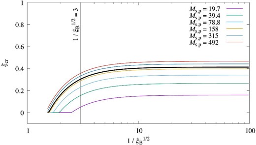
Maximum ξcr derived from f = 0 as a function of |$1/\sqrt{ \xi _{\rm B} }=v_0/(\delta B/\sqrt{4\pi \rho _0})$| for a given shock velocity v0 and T0 = 3 × 10⁴ K. The heavy black solid line shows |${\cal M}_{\rm s,p}=197$| (v0 = 4000 km s−1). The vertical thin line indicates |$1/\sqrt{ \xi _{\rm B} }=3$|. For a comparison, we display |${\cal M}_{\rm s,p}=$| 19.7 (purple, v0 = 400 km s−1), 39.4 (green, v0 = 800 km s−1), 78.8 (light blue, v0 = 1600 km s−1), 158 (orange, v0 = 3200 km s−1), 315 (blue, v0 = 6400 km s−1), and 492 (red, v0 = 10000 km s−1).
Figure 3 shows the results of downstream ion temperatures divided by 2Z (i.e., the particle mass in atomic units) for Model 0 and Model 3 with v0 = 4000 km s−1 and T0 = 3 × 10⁴ K. The reduced temperatures kTZ, z/2Z of Model 3 do not depend on the particle mass, indicating that the temperature ratios between the ions are equal to their ion mass ratio. Such mass-proportional ion temperatures are observed at SN 1987A (Miceli et al. 2019). The temperature jump Tj, 2/T0 is given by |$x_{{\rm c},j}/r_{\rm c}\sim {\cal M}_{{\rm s},j}$|. The relation of |$x_{{\rm c},j}/r_{\rm c}\sim {\cal M}_{{\rm s},j}$| is also implied by the condition of f = 0. Thus, Model 3 predicts that the ion temperature ratio is given by the mass ratio, similar to the case of Model 0. Note that Model 1 and Model 2 give ion temperatures almost the same as Model 0. On the other hand, kTZ, z/2Z of Model 3 is smaller than the case of Model 0 by a factor of 2 due to the generation of nonthermal components.
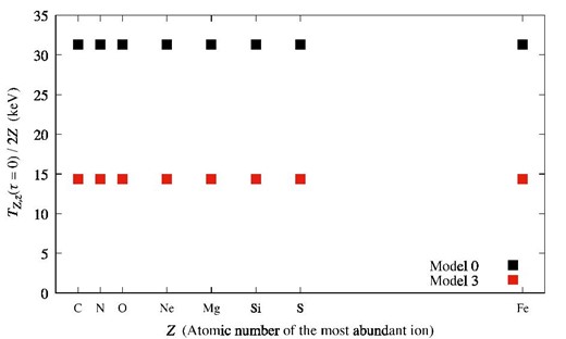
Initial downstream ion temperatures divided by 2Z (i.e., the particle mass in atomic mass units) for Model 0 and Model 3 with v0 = 4000 km s−1 and T0 = 3 × 10⁴ K. The black square shows the results of Model 0, and the red square shows the results of Model 3. The results of Model 1 and Model 2 are the same as the results of Model 0, respectively. The horizontal axis shows the atomic number Z.
Summary of the shock jump models.*
| Model | rc | kTp, 2 | kTe, 2 (β = Te, 2/Tp, 2) | ξB | ξcr |
|---|---|---|---|---|---|
| 0 | 4 | 31.32 keV | 17.1 eV (me/mp) | 0 | 0 |
| 1 | 4 | 31.01 keV | 31.0 eV (0.01) | 0 | 0 |
| 2 | 4 | 28.34 keV | 2.83 keV (0.1) | 0 | 0 |
| 3 | 3.29 | 14.38 keV | 8.62 eV (1.1me/mp) | 1/9 | 0.30 |
| 4 | 3.29 | 14.23 keV | 14.2 eV (0.01) | 1/9 | 0.30 |
| 5 | 3.29 | 13.01 keV | 1.30 keV (0.1) | 1/9 | 0.30 |
We set v0 = 4000 km s−1 and T0 = 3 × 10⁴ K. From the left-hand side to the right-hand side, the columns indicate the model name, the compression ratio rc, the downstream proton temperature kTp, 2, the downstream electron temperature kTe, 2, the fraction of the amplified magnetic field ξB = δB2/(4πρ0v02), and the fraction of the CR pressure ξcr = Pcr/(ρ0v02).
4 Evolution track of the downstream ionization balance and temperatures
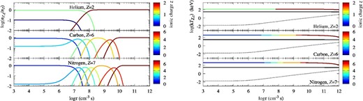
Ionization balance nZ, z/nZ (left) and temperature kTZ, z of the most abundant species among its ionic charge (right) for Model 0 with a shock velocity of v0 = 4000 km s−1. We display the species He, C, and N. The color represents the ionic charge z of the ion. The solid black line and black dots are the temperatures of the proton and electron, respectively.
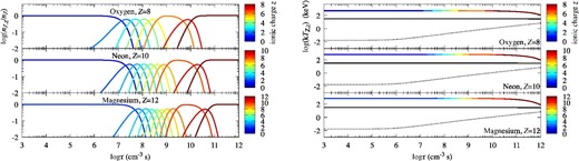
Ionization balance nZ, z/nZ (left) and temperature kTZ, z of the most abundant species among its ionic charge (right) for Model 0 with a shock velocity of v0 = 4000 km s−1. We display the species O, Ne, and Mg. The color represents the ionic charge z of the ion. The solid black line and black dots are the temperatures of the proton and electron, respectively.
Ionization balance nZ, z/nZ (left) and temperature kTZ, z of the most abundant species among its ionic charge (right) for Model 0 with a shock velocity of v0 = 4000 km s−1. We display the species Si, S, and Fe. The color represents the ionic charge z of the ion. The solid black line and black dots are the temperatures of the proton and electron, respectively.
The evolution tracks of nZ, z/nZ and TZ, z for other models are not so different from the case of Model 0. In the case of a higher electron temperature (Model 1 and Model 2), the ions are quickly ionized. Figure 7 shows the electron temperatures for Models 0, 1, 2, and 3 with v0 = 4000 km s−1. The relation between Model 4 and Model 1 (Model 5 and Model 2) is similar to that of Model 3 and Model 0. The ionization balance nZ, z/nZ becomes the same in each model after the electron temperature coincides. Note that the electron temperature increases within a column density scale of ntVsh ∼ 1014 cm−2(nt/106 cm−3 s)(Vsh/4000 km s−1). This column density scale is comparable to the size of the Hα emission region (e.g., Shimoda & Laming 2019). Therefore, to study the electron heating at the shock, the Hα observation may be better than the X-ray line observations. In the case of a lower ion temperature due to the production of Pcr and δB (Model 3), the temperature equilibrium is achieved at a smaller nt (e.g., the temperature of Fe is equal to that of the proton at nt ≃ 2 × 1011 cm−3 s) because the relaxation time of the Coulomb collision depends on T3/2 (Spitzer 1962). Note that the lower electron temperature results in a lower ionization state at a given τ ≃ nt.

Electron temperatures for Models 0 (black dots), 1 (purple dots), and 2 (green dots) with v0 = 4000 km s−1. The solid black line shows the proton temperature for Model 0. The red solid line and red dots are the proton and electron temperatures of Model 3, respectively.
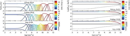
When the effects of the expansion become important, we cannot characterize the evolution only by τ ≃ nt and we should introduce parameters to describe the expansion of SNRs and the observed position r/Rsh(tage). Here we set ρ0 = 4.08 × 10⁻²mp, tage = 1836 yr, and Vsh(tage) = 3000 km s−1 for example. This parameter set will be used in comparisons of our model to the SNR RCW 86 (discussed later in section 5). Figure 8 shows the downstream ionization structure of He, C, N (top); O, Ne, Mg (middle); and Si, S, and Fe (bottom). The fluid parcel currently at r/Rsh(tage) = 0.8 crossed the shock at the time of t* when the shock velocity was Vsh(t*) = 5094 km s−1 for Models 0, 1, and 2 (4565 km s−1 for Models 3, 4, and 5). Since the compression ratio depends on whether the CRs exist, the shock transition time t*, shock velocity Vsh(t*), and Te(t*) are different for each model for the fluid parcel currently at r/Rsh(tage). The evolution of the ionization balance is similar to the case of the plane-parallel shock until t′ ∼ 109–1010 s ∼ tage. Cooling due to expansion becomes important at t′ ∼ tage. The ion temperatures decrease before the ions are well ionized due to the expansion (decreasing of the density, ion temperature, and electron temperature). Figure 9 shows the electron temperatures for Models 0 (black dots), 1 (purple dots), 2 (green dots), 3 (red dots), 4 (orange dots), and 5 (blue dots).
Ionization balance nZ, z/nZ for Model 0 with ρ0 = 4.08 × 10⁻²mp, tage = 1836 yr, Vsh(tage) = 3000 km s−1, and r/Rsh(tage) = 0.8. We display the species He, C, N (top); O, Ne, Mg (center); and Si, S, and Fe (bottom). The color represents the ionic charge z of the ion. The horizontal axis shows the time t′ = t − t*, where t* is the shock transition time of the fluid parcel currently at r/Rsh(tage) = 0.8.
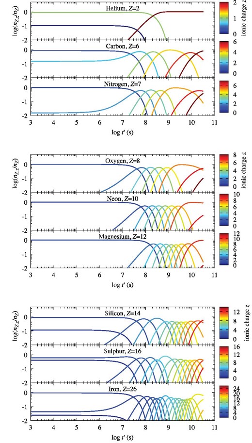
Electron temperatures for Models 0 (black dots), 1 (purple dots), 2 (green dots), 3 (red dots), 4 (orange dots), and 5 (blue dots) with ρ0 = 4.08 × 10⁻²mp, tage = 1836 yr, Vsh(tage) = 3000 km s−1, and r/Rsh(tage) = 0.8. The solid black (red) line shows the proton temperature for Model 0 (Model 3). The proton temperatures for Model 1 and Model 2 (Model 4 and Model 5) are almost the same as Model 0 (Model 3).
5 Synthetic observations
In this section, we perform synthetic observations of the shocked plasma considering the effects of turbulence for the case of the SNR RCW 86. Since we do not calculate the overall spectrum of the emitted photons, which needs enormous calculations about emission lines, we mainly estimate the line shape.
The SNR RCW 86 is one of the best targets for the study of CR injection via ion temperatures because the shells of the SNR show different thermal/nonthermal features from position to position (Bamba et al. 2000; Borkowski et al. 2001; Tsubone et al. 2017). RCW 86 is considered as a historical SNR of SN 185 (Vink et al. 2006). Thus, we set tage = 1836 yr. Along the north-eastern shell of RCW 86, the dominant X-ray radiation changes from thermal to synchrotron emission (Vink et al. 2006). The thermal emission-dominated region is referred to as the “E-bright” region, and the synchrotron one is referred to as the “NE” region. The ionization age at NE is estimated as τ = (2.25 ± 0.15) × 109 cm−3 s though this estimate potentially contains errors due to the lack of thermal continuum emissions (Vink et al. 2006). The E-bright region is fitted by two plasma components: (i) τ = (6.7 ± 0.6) × 109 cm−3 s, and (ii) τ = (17 ± 0.5) × 109 cm−3 s. Both E-bright and NE show clear O vii Heα and Ne ix Heα line emissions. From the width of the synchrotron-emitting region (NE), the magnetic-field strength is estimated as |$\approx \! 24\pm 5\,\, {\mu \rm {G}}$| (Vink et al. 2006).
Yamaguchi et al. (2016) measured proper motions around these regions (not exactly the same regions) as v0 = 720 ± 360 km s−1 (E-bright), v0 = 1780 ± 240 km s−1 (upper part of NE referred to as “NEb”), and v0 = 3000 ± 340 km s−1 (lower part of NE referred to as “NEf”). In the case of Model 3, the fractions of CR pressure ξcr become ξcr,720 ≃ 0.14 for v0 = 720 km s−1, ξcr,1780 ≃ 0.24 for v0 = 1780 km s−1, and ξcr,3000 ≃ 0.28 for v0 = 3000 km s−1, respectively. If we simply suppose ρ0 = (τ/tage)mp and adopt |$1/\sqrt{\xi _{\rm B}}=3$|, the CR pressure and δB of each region become Pcr,720 ∼ 0.2 keV cm−3 and |$\delta B_{\rm 720}\sim 51\,\, {\mu \rm {G}}$|, Pcr,1780 ∼ 0.3 keV cm−3 and |$\delta B_{\rm 1780}\sim 55\,\, {\mu \rm {G}}$|, and Pcr,3000 ∼ 1.1 keV cm−3 and |$\delta B_{\rm 3000}\sim 93\,\, {\mu \rm {G}}$|, where we adopt τ = 12.0 × 109 cm−3 s for the E-bright region as an average of the two components and τ = 2.25 × 109 cm−3 s for the NE region, respectively. If we adopt v0 = 360 km s−1 for the E-bright region, we obtain ξcr,360 ∼ 2.9 × 10⁻². The thermal-dominated E-bright region results from a higher density than the density at the NE region. The magnetic-field strengths δB are the almost the same as one another. Note that Vink et al. (2006) estimated the electron density at the E-bright region as ∼0.6–1.5 cm−3 from the emission measure assuming the volume of the emission region. Our model predicts the downstream density as rcρ0/mp ≈ 0.55 cm−3 for the E-bright region with v0 = 720 km s−1, which is consistent with the previous estimate. For the NE region, the number density is not well constrained because of the lack of the thermal continuum component. Thus, our choice of model parameters can be consistent with the observations of RCW 86. In the following, we apply our model to the NE region, setting the parameters as tage = 1836 yr, Vsh(tage) = 3000 km s−1, and ρ0/mp = τ/tage = 4.08 × 10⁻² cm−3, where τ = 2.25 × 109 cm−3 s is used. We suppose that the downstream region from r = Robs = 0.8Rsh(tage) to r = Rsh(tage) is observed. Then, our model supposes that the expansion follows the Sedov–Taylor model during a time of |$\Delta t\ge t_{\rm age}-t_*(R_{\rm obs}) = \left[1 - (R_{\rm obs}/R_{\rm sh})^{r_{\rm c}} \right] t_{\rm age}\approx 0.6\, t_{\rm age}$|, where rc = 4 and equation (11) are used. If RCW 86 expands with a velocity of ∼109 cm s−1 on average before entering the Sedov–Taylor stage, we effectively assume the radius at the transition time of t0 ≈ 0.6 tage as R0 ∼ 109 cm s−1 × 0.6 tage ∼ 11 pc. Then, the radius at the current time is Rsh(tage) ∼ R0(1/0.6)2/5 ∼ 13.5 pc, which can be consistent with the actual radius of ∼15 pc (the distance is assumed as 2.5 kpc).
Figure 10 shows the radial profile of the electron temperature at t = tage for Model 0 (black solid line), Model 1 (purple dots), Model 2 (green broken line), Model 3 (red solid line), Model 4 (orange dots), and Model 5 (blue broken line). To reproduce the bright O vii Heα, a relatively high electron temperature is preferred in terms of the excitation (∼1 keV; see also Vink et al. 2006), though it degenerates by the number density uncertainty. Note that the excitation rate is |$C_{\rm l,u}\propto \exp (-E_{\rm ul}/kT_{\rm e})/\sqrt{T_{\rm e}}$| and Eu, l ≃ 0.574 keV for O vii Heα. Thus, we mainly consider Model 2 (β = Te, 2/Tp, 2 = 0.1 without the CRs) and Model 5 (β = 0.1 with the CRs). Model 5 predicts kTe(r) ≃ 0.5 keV ≃ Eu, l; therefore the predicted O vii Heα line would be the brightest among the models.
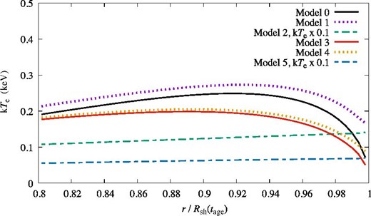
Radial profile of the electron temperature at tage = 1826 yr for the NE region of RCW 86 with Vsh(tage) = 3000 km s−1 and ρ0/mp = 1.29 × 10⁻². We display the results of Model 0 (black solid line), Model 1 (purple dots), Model 2 (green broken line), Model 3 (red solid line), Model 4 (orange dots), and Model 5 (blue broken line).
Figure 11 shows the radial profile of the oxygen abundance nZ, z/nZ for Model 2 (left) and Model 5 (right). The O vii abundance (orange) is large. Note that the other models (e.g., Model 0) also result in a large O vii abundance. Model 2 predicts a smaller abundance of O vii than the case of Model 5 because the higher electron temperature results in faster ionization. The temperature of O vii is approximately kTZ, z(r) ≈ 250 keV × [r/Rsh(tage)] for Model 2 and kTZ, z(r) ≈ 140 keV × [r/Rsh(tage)] for Model 5.
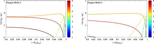
Radial profile of the oxygen abundance nZ, z/nZ at tage = 1826 yr for the NE region of RCW 86 with Vsh(tage) = 3000 km s−1 and ρ0/mp = 1.29 × 10⁻². The left panel shows the results of Model 2 and the right panel shows Model 5. The color indicates the ionic charge z of the ion.
Figure 12 shows |$I_\nu ({\cal X})/I_\nu (0.8\, R_{\rm sh})$| at the line center for Model 5 (solid lines) and Model 2 (dots). We also display profiles of the column density of O vii (green). The difference between the column density profile and the intensity profile results from the excitation. The spatial variation of the electron temperature is relatively less important in this case because the excitation rate depends on |$\exp (-E_{\rm ul}/kT_{\rm e})/\sqrt{T_{\rm e}}$|, which is not so sensitive to Te unless kTe ≪ Eul.
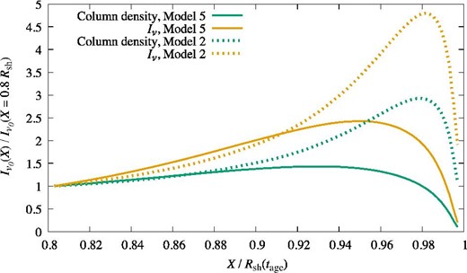
Radial profile of the specific intensity |$I_\nu ({\cal X})/I_\nu (0.8R_{\rm sh})$| at the line center for O vii Heα (orange). The solid lines show the results of Model 5 (multiplied by a factor of 10) and the dots show Model 2. We also display profiles of the column density (green) of O vii.
Figure 13 shows the calculated O vii Heα line for Model 5 (blue solid line) and Model 2 (green solid line) derived from |$\int I_\nu d{\cal X}$| with δ = 0.5. We assume the distance of RCW 86 as 2.5 kpc (Yamaguchi et al. 2016) and the observed area as 0.2Rsh × 0.2Rsh, where Rsh = 15.27 pc. We also display the results of Model 0 (black dots), Model 1 (purple dots), Model 3 (red dots), and Model 4 (orange dots). The results show a good agreement with the observed photon counts ∼0.15 counts s−1 keV−1 (Vink et al. 2006). Table 3 shows a summary of the calculated O vii Heα line. The derived temperatures reflect the effects of the efficient CR acceleration. From the comparison of δ = 0.5 to δ = 0, turbulent Doppler broadening results in higher observed temperatures by a factor of ∼1.05. The degree of broadening can be estimated as |$\sqrt{1+{\cal M}_{Z,z}{}^2}\approx 1.1$| for δ = 0.5 with approximating Tp/TZ, z ≈ mp/mZ. Since the observed line consists of multiple temperature populations, and since a higher-temperature population contributes less around the line center, a lower-temperature population is accentuated around the line center. The contribution of the higher-temperature population appears far from the line center like a “wing.” If we measure the temperature using the full width at the e-folding scale, the difference in the derived temperatures becomes large. Hence the observed FWHM is smaller than that expected from |$\sqrt{1+{\cal M}_{Z,z}{}^2}$|.

Calculated O vii Heα line with δ = 0.5 for Model 5 (blue solid line) and Model 2 (green solid line). We also display the results of Model 0 (black dots), Model 1 (purple dots), Model 3 (red dots), and Model 4 (orange dots). We assume that the distance of RCW 86 is 2.5 kpc and the observed area is 0.2Rsh × 0.2Rsh, where Rsh = 15.27 pc.
Summary of the calculated O vii Heα.
| kTZ, z (kTZ, z/2Z)* | ||
|---|---|---|
| Model | for δ = 0.5 | for δ = 0 |
| 0 | 325.9 keV (20.4 keV) | 312.3 keV (19.5 keV) |
| 1 | 325.6 keV (20.3 keV) | 312.4 keV (19.5 keV) |
| 2 | 306.4 keV (19.2 keV) | 296.5 keV (18.5 keV) |
| 3 | 160.6 keV (10.0 keV) | 153.8 keV (9.62 keV) |
| 4 | 160.6 keV (10.0 keV) | 154.2 keV (9.63 keV) |
| 5 | 157.7 keV (9.85 keV) | 152.5 keV (9.53 keV) |
The O vii temperature derived from the FWHM of the line for the case of δ = 0.5 and δ = 0.
RCW 86 also shows bright Ne ix Heα; however, our model predicts a faint Ne ix Heα emission (the intensity is smaller than a tenth of the O vii Heα intensity). The line intensity also depends on the ion abundance. In this paper, we use the solar abundance, which reflects the condition of our Galaxy ≃4.6 Gyr ago. Moreover, De Cia et al. (2021) found large variations in the chemical abundance of the neutral ISM in the vicinity of the Sun over a factor of 10 (they analyzed Si, Ti, Cr, Fe, Ni, and Zn). Their findings imply that the gaseous matter is not well mixed. The predicted faint Ne ix Heα might reflect a different abundance pattern from the solar abundance pattern.
Figure 14 represents the line shape with 5 eV resolution for δ = 0.5. We additionally show O vii Lyα, Ne ix Heα, and Ne x Lyα. Since the widths of the particle distribution function are almost the same as each other for nt ∼ 109–1011 cm−3 s, the observation of lines at higher photon energies is better to resolve the line width. Note that the observed O vii Heα and Ne ix Heα are bright compared to the continuum emission (Vink et al. 2006). The energy resolution of XRISM’s micro-calorimeter Resolve is sufficient to distinguish whether the SNR shock accelerates the CRs (Model 5) or not (Model 2).

Line profiles with 5 eV resolution for δ = 0.5. We display O vii Heα, O viii Lyα, Ne ix Heα, and Ne x Lyα for Model 5 (black solid line) and Model 2 (green solid line).
6 Summary and discussion
We suggest a novel collisionless shock jump condition, which is given by modeling each ion species’ entropy production at the shock transition region. As a result, the amount of the downstream thermal energy is given. The magnetic-field amplification driven by the CRs is assumed. For a given strength of the amplified field, the amount of CRs is constrained by the energy conservation law. The constrained amount of CRs can be sufficiently large to explain the Galactic CRs. The ion temperature is lower than the case without CRs because the upstream kinetic energy is divided into CRs and the amplified field. The strength of the field around the shock transition region is assumed to be |$1/\sqrt{\xi _{\rm B}}=v_0/(\delta B/\sqrt{4\pi \rho _0})\simeq 3$|. Downstream developments of the ionization balance and temperature relaxation are also calculated. Using the calculated downstream values, we perform synthetic observations of atomic lines for the SNR RCW 86, including Doppler broadening by turbulence. Our model predictions can be consistent with previous observations of the SNR RCW 86, and the predicted line widths are sufficiently broad to be resolved by XRISM’s micro-calorimeter. Future observations of the X-ray lines can distinguish whether the SNR shock accelerates the CRs or not from the ion temperatures.
Our shock model constrains the maximum fraction of the CRs depending on the shock velocity, the upstream density, and the sonic Mach number (see figure 2). Since the SNR shock decelerates gradually, we can predict the history of the CR injection and related nonthermal emissions, especially the hadronic γ-ray emissions. Although the injection history of the CRs is essential to estimate the intrinsic injection of the CRs into our Galaxy per one supernova explosion, this issue currently remains to be resolved (e.g., Ohira et al. 2010; Ohira & Ioka 2011). The injected CRs will contribute to the dynamics of the ISM as a pressure source, leading to a feedback effect on the star formation rate, for example (e.g., Girichidis et al. 2018; Hopkins et al. 2018; Shimoda & Inutsuka 2022). The origin of γ-ray emissions in the SNRs is also unsettled, whether of hadronic origin or leptonic origin (Abdo et al. 2011; but see also Fukui et al. 2021). We will study these in a forthcoming paper.
For distinguishing the case of extremely efficient CR acceleration (Model 3) from the case of no CRs (Model 0), a comparison of the FWHM to other values is required in general (e.g., the difference between the ionization states, the shock velocity, and so on). The FWHM of Model 3 becomes smaller than Model 0 at a given shock velocity and nt, and abundant ions of Model 3 tend to be less ionized than in the case of Model 0 because of the lower electron temperature. The lower electron temperature and lower ionization states of Model 3 may result in a different photon spectrum from the case of other models, especially the equivalent widths, recombination lines, Auger transitions due to inner shell ionization, and so on. We will attempt further investigations by calculating the overall photon spectrum in future work.
The line diagnostics of the thermal plasma of young SNRs on the effect of CR acceleration will be a good science objective for the XRISM mission (Tashiro et al. 2020), which will provide high-resolution X-ray spectroscopy. Since the micro-calorimeter array is not a distributed-type spectroscope like grating optics on Chandra and/or XMM–Newton, the Resolve onboard XRISM (Ishisaki et al. 2018) can accurately measure the atomic line profiles in the X-ray spectra from diffuse objects like SNRs. XRISM will have an energy resolution of 7 eV (as the design goal), and the calibration goals on the energy scale and resolution are 2 eV and 1 eV, respectively (Miller et al. 2020). Therefore, the line broadening values from multiple elements with/without CRs in figure 3 can be distinguished by XRISM. Another importance of XRISM is the wider energy coverage, with which atomic lines not only from light elements (C, N, O, etc.) but also from Fe will be measured. So, the intensity of the turbulence demonstrated in section 5 will be constrained with XRISM. The preparations for the instruments (Nakajima et al. 2020; Porter et al. 2020) and in-orbit operations (Loewenstein et al. 2020; Terada et al. 2021) are proceeding smoothly for the launch in 2022/2023, and several young SNRs, including RCW 86, are listed as targets during the performance verification phase of XRISM.5 We expect to verify our predictions observationally soon.
Acknowledgements
We thank K. Masai and G. Rigon for useful discussions. We are grateful to the anonymous referee for his/her comments, which further improved the paper. This work is partly supported by JSPS Grants-in-Aid for Scientific Research Nos. 20J01086 (JS), 19H01893 (YO), JP21H04487 (YO) 19K03908 (AB), 20K04009 (YT), 18H01232 (RY), 22H01251 (RY), and 20H01944 (TI). YO is supported by the Leading Initiative for Excellent Young Researchers, MEXT, Japan. RY and SJT deeply appreciate the Aoyama Gakuin University Research Institute for helping our research with the fund.
Footnotes
The compression ratio is strictly a function of the shock velocity. For the calculation of t* only, we use the compression ratio given by Vsh(tage) but, for the other cases, we calculate the shock jump conditions using Vsh(t*) given by the calculated t*.
This definition corresponds to a reversible process. The collisionless shock is formed by the wave–particle interaction, which might be a reversible process like a plasma echo, for example. Although this may be an unsettled issue, we apply this definition of entropy in this article. Note that the entropy is defined as a non-dimensional value differing from the usual dimensional definition in thermodynamics, dS = dQ/T.
