


Abstract
Detecting and tracking objects in low Earth orbit is an increasingly important task. Telescope observations contribute to its accomplishment, and telescope imagers produce a large amount of data for this task. Thus, it is convenient to use fast computer-aided processes to analyze it. Telescopes tracking at the sidereal rate usually detect these objects in their imagers as streaks, their lengths depending on the exposure time and the slant range to the object. We have developed a processing pipeline to automatically detect streaks in astronomical images in real time (i.e., faster than the images are produced) by a graphics processing unit parallel processing system. After the detection stage, streak photometric information is obtained, and object candidate identification is provided through matches with a two-line element set database. The system has been tested on a large set of images, consisting of two hours of observation time, from the Tomo-e Gozen camera of the 105 cm Schmidt telescope at Kiso Observatory in Japan. Streaks were automatically detected in approximately 0.5% of the images. The process detected streaks down to a minimum apparent magnitude of +11.3 and matched the streaks with objects from the space-track catalog in 78% of the cases. We believe that this processing pipeline can be instrumental in detecting new objects and tracking existing ones when processing speed is important, for instance, when a short handover time is required between follow-up observation stations, or when there is a large number of images to process. This study will contribute to consolidating optical observations as an effective way to control and alleviate the space debris problem.
1 Introduction
The growth in the population of objects in Earth orbits, especially in low Earth orbit (LEO), has increased during the last few years, making detecting and tracking them more challenging for space surveillance systems. Space surveillance can be done through optical observations, where images produced by telescope cameras can be processed to search for these objects. Formerly this work was performed by technicians, but soon the convenience of automating this process was noted, allowing a large volume of images to be quickly processed and at low cost (Leu 1992). Nowadays, large-capacity digital storage devices capable of storing massive amounts of images to process challenge the capacity of hardware and software computing resources. Furthermore, when several observation sites are used, the orbital parameters of an object detected in one of them need to be sent to an observation site quickly for a follow-up. These reasons justify the exploration of fast and efficient ways to locate Earth-orbiting objects in astronomical images automatically.
Telescopes tracking at the sidereal rate usually detect Earth-orbiting objects as elongated shapes or streaks with lengths that depend on the exposure time of the imager and the slant range to the object. In a computer vision application, algorithms frequently detect streaks in images by performing the same operations over a high number of pixels. If we want to speed up the processing time, parallel processing is a sensible paradigm to choose. CPU-based processing is optimized for sequential operations and multicore CPU systems help process the same tasks in parallel as soon as tasks reach a certain complexity. In pixel-based processing of images, a simple set of operations is usually required, such as thresholding, kernel filtering, adding, or subtracting. These operations are performed over a massive number of pixels, and this is where graphics processing unit (GPU)-based processing can show a dramatic improvement in processing speed over CPU-based processing, as shown in Niwano et al. (2021), where they increased the processing speed of an astronomical image reduction pipeline by more than 40 times when they added GPU-based processing to the original pipeline.
A processing pipeline to detect streaks in astronomical images can be structured in three stages: preprocessing, where images are prepared to maximize the detection rate in the next stage; detection, where the actual streak detection algorithm is run and the output is streaks located by their x–y image plane coordinates; and postprocessing, where the astrometric coordinates and apparent magnitude can characterize streaks, or can be associated with a real object when its coordinates match an entry in a two-line element set (TLE)-based database.
The literature shows that most researchers have followed the previous stages, introducing various methods and algorithms in each of them. The common aim was to make the process as efficient as possible, usually to detect very faint streaks or to reduce the number of false positives (detected streaks that do not correspond to real objects).
In the preprocessing stage, raw images from the camera are processed so that the next stage can maximize the number of detectable streaks. This can include eliminating dead pixels and image artifacts, detecting and removing the background, removing stars, and binarizing the image. In this stage, subtracting dark frames and flat-fielding can reduce the large-scale background from the raw images. Levesque (2009) used an iterative background removal method through clipping the local statistics values in the images, and Oniga et al. (2011) used an exponential moving average technique, which also removed stars from the raw image. Cvrček and Šára (2019) subtracted a simulated background image from the raw image using cataloged stars.
Removing stars helps reduce the false positives created by the bright stars’ diffraction spikes, which can be mistaken for real objects. One method is median stacking (Yanagisawa et al. 2005), which is the approach followed in the present work and is explained in section 2. Another preprocessing method uses image moments to classify objects as rounded or elongated, so the rounded ones can be discarded so that only the ones with streaks are left (Wallace et al. 2007).
The detection stage applies an algorithm to detect linear shapes in the preprocessed image generated in the previous stage. This stage aims to end up with a list of streak candidates, each characterized by a pair of x–y coordinates corresponding to the ends of the streaks in the image. Usually, this stage consists of an algorithm that provides information about streak-like shapes in the image, followed by a process to reduce this information to the x–y coordinates of the beginning and end of the candidate streak. This yields a position as close as possible to the object’s position at the beginning and end of the exposure time of the imager.
In the literature, researchers have applied variations of different techniques to detect streaks, such as the Hough transform (HT) (San Martin et al. 2020), the Radon transform (Ciurte & Danescu 2014; Nir et al. 2018; Hickson 2018; San Martin et al. 2020), the distance transform (Diprima et al. 2017), pixel connectivity (Wallace et al. 2007; Haussmann et al. 2021), matched filters (Levesque 2009; Cvrček & Šára 2021), and labeling (Oniga et al. 2011). Some authors have applied statistical methods, such as Cvrček and Šára (2019), where a binary decision (i.e., the presence or absence of streaks in the image) is made based upon statistical parameters, in what they call a streak certification process, or Dawson, Schneider, and Kamath (2016), who used a maximum likelihood estimation method.
The postprocessing stage characterizes the streaks to obtain real information on the object that creates the streak. In this stage, several processes can occur: elimination of false positives, conversion of x–y coordinates to astronomical coordinates, streak photometric measurement, or identification by comparing astronomical coordinates with orbital coordinates of already cataloged objects, usually through their TLE information.
In the above literature, the authors have mainly focused on increasing the system’s sensitivity, so fainter streaks are detected, even ones not visible to the human eye, and decreasing the number of false positives. Nevertheless, only a few have focused on decreasing the processing time. Diprima et al. (2017) have applied GPU technology, reporting a mean processing time of 3.19 s for an image of 4096 × 4096 pixels (an improvement of 7.3 times over its CPU version). Without using a GPU, Zimmer, McGraw, and Ackermann (2015) reported a time of 0.9 s per 2 × 2 binned image of 4864 × 3232 pixels, the preprocessing of which took 0.4 s and detection 0.5 s. Other researchers have reported the next timing results: Cvrček and Šára (2019) reported a time of 2–7 min per 2049 × 2047 (16-bit) image, depending on the SBR (signal-to-background ratio) of the streak; Hickson (2018) reported a 3 s processing time for a 1 × 1 K image, 10 s for a 2 × 2 K image, and 30 s for a 4 × 4 K image; Tagawa et al. (2016) reported a time frame of several minutes for a set of 18 2 × 2 K images; the approach of San Martin et al. (2020) took 3–4 hr to process a 4 × 4 K image in MATLAB; and Virtanen et al. (2016) reported a 13 s processing time for a 2 × 2 K image.
There is usually a tradeoff between processing speed and detectability rate in the detection process. A sensitive algorithm could be efficient in detecting streaks even below the background noise of the image, but its processing speed might be too large for processing thousands of images and vice versa. We chose a compromise between speed and detectability rate in the present work, achieving what we can call “real-time” performance. For the discrete process of creating image files by a telescope system, for our work we consider that the meaning of “real-time” is equivalent to detecting streaks faster than the image files are produced.
In our work, the processing pipeline also consists of the three stages mentioned earlier: preprocessing, detection, and postprocessing. Section 2 describes the system hardware, including the CPU and GPU specifications and the GPU’s parallel processing pipeline. Section 3 describes preprocessing, which includes star removal based on a median stack and image binarization. Section 4 outlines the detection process, which consists of a GPU implementation of the progressive probabilistic version of the classical HT technique to detect linear shapes in images. In section 5, the postprocessing stage is described, which obtains the astrometric and photometric measurements of the streaks, and also a list of possible real object candidates through the comparison with a TLE database of objects in orbit. Section 6 describes the experimental setup. Finally, the research results and conclusions are presented in sections 7 and 8, respectively.
2 Parallel processing implementation
Current medium-range computers usually have CPUs with multiple cores that can provide parallel processing. In this work, we used a set of four parallel CPU–GPU threads, as shown in figure 1, in a computer with four GPU cards connected through a multicore CPU. Table 1 shows the main specifications of this CPU–GPU computing system. Four files are processed in parallel in four CPU cores, and for each file, sequential tasks are executed in the CPU, while pixel-level operations are executed in the GPU.
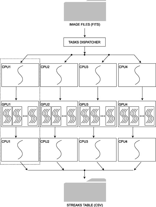
Parallel processing hardware configuration: The task dispatcher serves the image file to four different threads (CPU1–GPU1, CPU2–GPU2, CPU3–GPU3, CPU4–GPU4). Processes are represented as curved lines, which are executed sequentially in each CPU and in parallel in each GPU. The computations in the four threads are combined in one unique output csv file.
CPU–GPU system specifications.
| CPU | |
|---|---|
| Model | Intel core i9-10940X 3.30 GHz |
| Cores/threads | 14/28 |
| RAM memory | 128 GB DDR4 |
| GPU (×4)* | |
| Model | Nvidia Quadro RTX8000 |
| Number of cores | 4608 |
| Memory | 49 GB |
| Bus type | PCI Express ×16 Gen.3 |
| CPU | |
|---|---|
| Model | Intel core i9-10940X 3.30 GHz |
| Cores/threads | 14/28 |
| RAM memory | 128 GB DDR4 |
| GPU (×4)* | |
| Model | Nvidia Quadro RTX8000 |
| Number of cores | 4608 |
| Memory | 49 GB |
| Bus type | PCI Express ×16 Gen.3 |
Specifications per GPU card unit.
Figure 2 shows in detail the process in one CPU–GPU thread (indicated by a dashed rectangle in figure 1). The original image file consists of consecutive images taken with a camera without latency and stored as a flexible image transport system (FITS) image file of three dimensions. The CPU first converts the previous image file to a two-dimensional image file and stores it in RAM because the libraries with functions to process image files at the pixel level in this algorithm are designed to manage only two-dimensional images. Then the CPU transfers the flattened image file from CPU memory to GPU memory (global memory). Once the image is loaded in the global memory, the runtime CUDA routine applies the Hough algorithm to each pixel, processing one pixel per thread, distributed in several multiprocessors (MP). Each of the MPs creates a list of coordinates for each subframe of the image, and these data are stored internally in global memory. After this, the GPU routine transfers this list to CPU memory; it is eventually saved as a csv file that can later be stored and read by the computer’s OS.
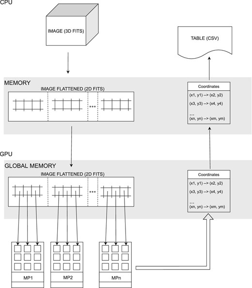
Single CPU–GPU thread pipeline: Arrows represent data transfers between different blocks of the CPU (top) and the GPU (bottom). Data transfers within the CPU and from CPU memory to GPU memory are sequential, whereas data transfers within the GPU, between GPU memory and multiprocessors, are executed in parallel.
3 Preprocessing stage
This stage has two steps: star removal and image binarization. Star removal helps eliminate the false positives created when diffraction spikes of bright stars appear in images. Image binarization eases the computational overhead of the detection stage, as it operates over Boolean values instead of floating-point values. Figure 3 shows the steps of this process on a sample image.
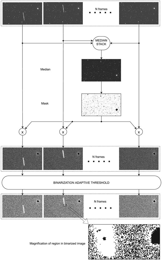
Preprocessing stage: This process starts at the top with N consecutive frames. After multiplication with the median stack mask, the stars are removed from these frames, and then, after adaptive thresholding, the frames are binarized. A magnification of a binarized image is shown at the bottom of the figure.
3.1 Star removal
To remove the stars from an image, we apply a variation of the median stacking method (Yanagisawa et al. 2005) over consecutive images. First, a median value is calculated for each pixel of the stack of images with the same location. This way, moving objects, such as streaks, disappear in the median stacking image because their positions are different in each image. In contrast, stationary objects, such as stars, keep their value. Once we obtain the median image of the stack (median stack in figure 3), we create a mask. In Yanagisawa et al. (2005), the median stack is subtracted from each of the series of images applying a threshold with a value slightly higher than the median value of the median image. The lengths of the diffraction spikes of the stars will vary with both their magnitude and the telescope optics, so the threshold value should be chosen accordingly. In the experimental setup of this work, explained later in section 6, we chose a threshold value of 1.3 times the mean value of the median stack, which was enough to remove the diffraction spikes of the brighter star of the region of the sky covered in the observation run, considering the optical properties of the telescope and camera used in the experiment. Pixels above this threshold are assigned 0, whereas pixels below keep their original values. Then we multiply the original image pixel by pixel with this mask, so zeros replace the pixels with stars, and only moving objects are visible in the final image.
3.2 Image binarization
In this step, the image is binarized; that is, its brightness is converted to ones and zeros, which simplifies and speeds operations over the pixels in the detection stage. Binarization of the image can be applied globally to the whole image with a specific threshold value or locally through adaptive thresholding. The global thresholding technique uses the same value for all pixels of the image, whereas adaptive thresholding considers a small set of neighboring pixels around each pixel of the image to compute the thresholding value; therefore this value is “adapted” to small regions of the image. This technique can be useful when applied to astronomical images, as these can have non-uniform illumination across the image, due to weather conditions, atmosphere turbulence, or the existence of very bright objects in the image, among others. In our work, we apply this technique so that we can detect faint streaks than could otherwise be masked if we apply global thresholding. Figure 3 (bottom) shows the result for an example image after the adaptive binarization thresholding has been applied to images with the stars already removed.
4 Detection stage
The detection stage locates lines that are candidates for belonging to a streak in an image, and then it determines the x–y coordinates of the ends of the streak, finding the longest segment that belongs to the streak. Figure 4 shows the steps to obtain the coordinates of the streak ends.
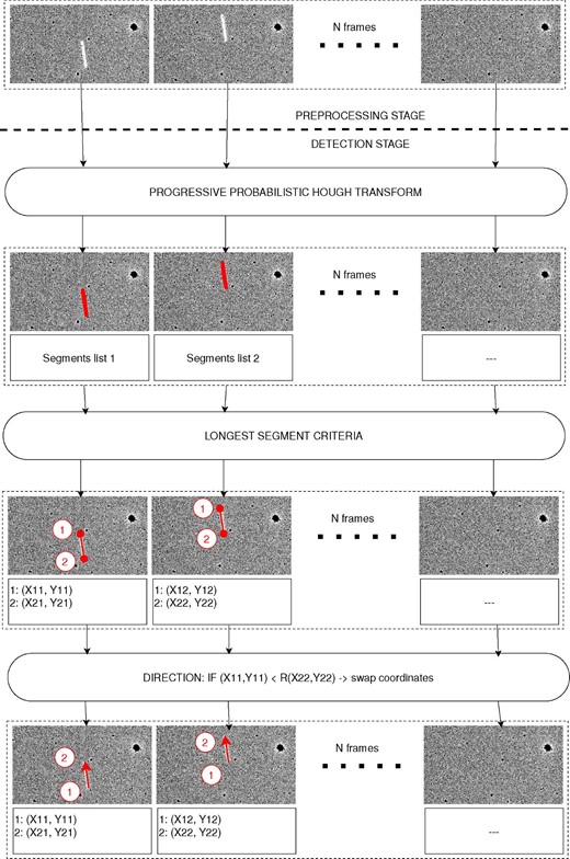
Detection stage: From top to bottom, after the preprocessing stage, PPHT is executed and the segments are detected (in red). Then, after applying the longest segment criteria, coordinates of both ends of the streaks are obtained (1 and 2). In the last step, the streak direction is obtained comparing the end coordinates of the streak in consecutive frames.
As mentioned in the introduction, there are several methods to detect linear shapes in images, including HT, the Radon transform, and matched filters. The literature has reported some GPU implementations of HT to detect linear shapes. Braak (2011) showed several implementations, where the fastest version showed an improvement of 10× over simpler GPU algorithm versions. These GPU implementations showed a 7× speed increase over the CPU version of the transform. In Bazilinskyy (2012), the GPU implementation showed a 4× processing speed improvement over the CPU version. The author concluded that the number of threads in the GPU did not affect the performance. In Yam-Uicab (2017), the authors presented several HT implementations on a GPU, showing a 20× timing performance over the CPU version. We see that, for HT, GPU processing generally significantly reduces the processing time compared to CPU processing, although the improvement depends on the image size and the particular model of the GPU card.
HT consists of applying the same simple arithmetic operations (accumulation) to each pixel, transforming each coordinate from x–y to polar coordinates, and counting the number of votes to find the candidates that belong to a particular linear shape. As these operations have to be repeated over many pixels, it seems appropriate to use one processing thread per pixel in a parallel GPU system so that HT benefits the GPU processing pipeline.
HT was devised and patented by Paul Hough in 1962.1 Since then, it has undergone many variations and improvements. In the progressive Hough transform (PHT) (Kiryati et al. 1991), using only a fraction of the input points in the voting process makes it possible to obtain the same results as in HT but much faster. Matas, Galambos, and Kittler (2000) presented a variation of PHT, called the progressive probabilistic Hough transform (PPHT), which is the one that we used in the present work.
PPHT provides two crucial advantages in our work: shorter processing time and segment detection instead of line detection. Apart from the previous advantages, GPU software libraries of PPHT implementations are already well maintained and reliable and can be easily integrated with the rest of our processing pipeline. OpenCV is an open-source computer vision library that has been available since 2000 under the BSD open-source license, and in 2010 a module was added that provided GPU acceleration capabilities. In our work, we use a function of this library (cv:: cuda:: createHoughSegmentDetector) that implements PPHT. The PPHT OpenCV function has several parameters to adjust its behavior, and table 2 summarizes them with the values that we adopted for our processing pipeline.
Parameters of function create Hough Segment Detector.*
| Parameter | Description | Value |
|---|---|---|
| ρ | Distance resolution (pix) | 1 |
| θ | Angle resolution (radians) | π/180 |
| minLineLength | Minimum line length (pix) | 200 |
| maxLineGap | Maximum allowed gap (pix) | 1 |
| MaxLines | Maximum no. output lines | 1000 |
| Parameter | Description | Value |
|---|---|---|
| ρ | Distance resolution (pix) | 1 |
| θ | Angle resolution (radians) | π/180 |
| minLineLength | Minimum line length (pix) | 200 |
| maxLineGap | Maximum allowed gap (pix) | 1 |
| MaxLines | Maximum no. output lines | 1000 |
The chosen values of ρ and θ guarantee that we detect all possible angles in the streaks regardless of the pixel size. We defined a minimum length of 200 pixels (minLineLength = 200), the minimum needed to detect streaks reliably, as shorter lengths can cause the system to generate false positives. We used a restrictive number of one pixel as the maximum allowed gap between points of the same line, thus avoiding random noise in the image that appears as lines and could be incorrectly detected as streaks.
Figure 5 shows the result of the detection stage, in which the output is represented as segments superimposed over the real streaks, on two sample astronomical images. The number of segments detected per streak depends on the streak width and the noise in the image. In the left image of figure 5, only 10 segments were detected, whereas, in the right image, 200 segments were detected.
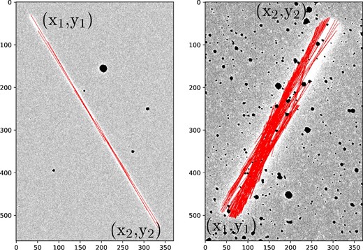
Detection stage: segments detected with the PPHT transform, 10 segments in the left figure, 200 segments in the right figure. Segments are represented in red, superimposed over the original image with the stars removed (0 values).
The output of the detection algorithm is a list of segments defined by two coordinates each, corresponding to each end. The longest of these segments most closely approaches the actual shape of the streak, so the algorithm will determine these longest segments under the assumption that their coordinate ends are the coordinates that characterize the streak. This assumption works well in most cases, but in a few cases, when a bright star and the streak overlap, the end coordinates could not correspond to the actual ends of the streak because the longest segment would not cover the entire length of the streak, and this could lead to a wrong identification of the object that created the streak.
After the detection stage, the algorithm generates a table that lists all detected streaks and their end coordinates in the x–y image plane.
5 Postprocessing
The postprocessing stage consists of a series of tasks to characterize the detected streak: RA and Dec (astronomical coordinates), photometric measurements (to characterize the sensitivity of the system with apparent magnitude values, so it is not included in the processing pipeline), and identification of the object that created the streak. This last step is done by comparing the coordinates of the ends of the streak with those of known objects in a database based on the orbital propagation of their initial TLE coordinates. Usually, the postprocessing stage is slower than preprocessing and detection. Still, we must consider that these latter stages are executed over all the images. In contrast, postprocessing is run only on images with candidate streaks, usually a small percentage of the images.
5.1 Astrometry
If the provided images already contain astrometric calibration information (the World Coordinate System, WCS), we can use some of the libraries that transform x–y to RA/Dec coordinates, such as the WCSTools library.2 This software uses the WCS information in the FITS file header and computes the RA/Dec coordinates with high precision. The advantage of this software is that it can be invoked from the command line, which makes integration with the main processing pipeline easy without extra user interaction. The coordinates of the detected streak ends are used for this conversion.
If the WCS information is not included, we first execute a plate solve calculation that provides the RA/Dec coordinates of the streak’s ends. However, this penalizes the processing time, as the plate solve process is not usually quick. To do a plate solve integrated into the general processing pipeline, we use the application program interface (API) of the astrometry.net project (Lang et al. 2010). Calling the API function “solve-field” with the appropriate parameters writes the FITS file header with WCS information that will later be used by the WCSTools library to obtain the RA/Dec coordinates of the streak ends.
5.2 Photometry
To further characterize the streaks, the photometric values of the streaks were measured. This process did not use the main processing pipeline and was applied only to evaluate the sensitivity of the detection process so that it could be compared with other processing pipelines. The apparent magnitude obtained cannot be interpreted as an intrinsic feature of the object that created the streak (as is done in traditional astronomical photometry). The apparent magnitude value depends on many factors, such as elevation, object shape configuration (planar, spherical), and phase angle. In our work this process was intended to measure the sensitivity of the process when used with a particular telescope and camera.
To integrate the photometry calculation with the processing pipeline, we used the Python packages Astroquery (Ginsburg et al. 2019) and Photutils.3 The steps that the algorithm follows are outlined next:
Calculate the counts encircled by an ellipsoidal area surrounding the streak.
Obtain sources within the image with the command DAOStarFinder of the Photutils software package.3
Convert the x–y coordinates of the streak ends to RA/Dec.
Convert the x–y coordinates of each image corner to RA/Dec.
Generate a query in the Gaia database to find photometric stars in the image. This query obtains a table with photometric stars in the area, with their measured apparent magnitudes.
Associate each value of a source with its corresponding photometric star from the Gaia database query according to the following criteria:
If (RA(source) - RA(star) < 0.002)
AND (Dec(source) - Dec(star) < 0.002)
THEN (source = photometric star)
Calculate a photometric table with values of sources identified as photometric stars executing the function aperture_photometry of the Photutils software package.3
- For each photometric value in the previous results, calculate the instrumental magnitude using the number of counts in each aperture of photometric stars:(1)$$\begin{equation} (-2.5) \times \log _{10} \ (\mathrm{star\_counts}) \end{equation}$$
- Calculate the instrumental magnitude of the streak using the number of counts within the ellipse surrounding the streak:(2)$$\begin{equation} (-2.5) \times \log _{10} \ (\mathrm{streak\_counts}) \end{equation}$$
Perform a least-squares polynomial fit with the Python function np.polyfit from the Numpy software package between the apparent magnitudes of sources and previous instrumental magnitudes. The result of the polynomial fit is the apparent magnitude of the streak and the residual error, that is, an indication of the precision of the apparent magnitude of the streak.
Figure 6 shows an example of an ellipsoidal area programmatically selected that surrounds both ends of the streak used to calculate the number of counts in the streak, and the photometric stars used to execute the differential photometry.
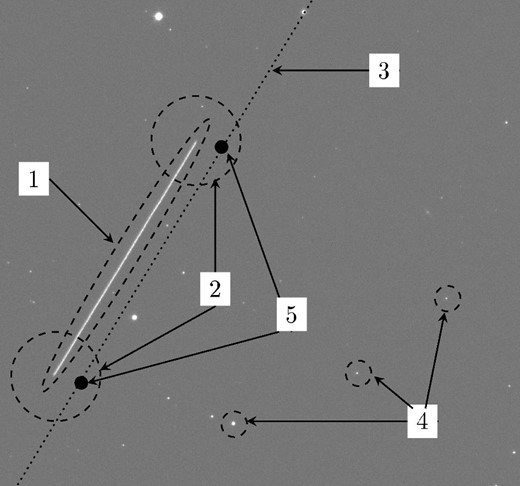
Postprocessing stage: (1) The elliptical area surrounding the detected streak to compute the total brightness. (2) Circular areas surrounding both ends of the detected streak, which define the error with the TLE database of object comparison. (3) The trajectory of the real object in the database obtained through the propagation of its TLE data with the SGP4 algorithm. (4) Photometric stars. (5) (RA, Dec) coordinates of an object from the database corresponding to the timestamps of the start and end of camera integration time. If these points are encompassed by the circular areas (2), the streak is associated with the candidate object.
5.3 Identification
This step compares the RA/Dec coordinates of each element of a large database of known objects for starting and ending exposure times in the camera with the RA/Dec coordinates of the streak ends. The database is obtained by downloading their respective TLE files and calculating their coordinates applying a standard general perturbations satellite orbit model 4 (SGP4) algorithm. If the distance between those coordinates is below a specific range (depending on the pixel scale of the camera), we categorize that object as having generated the streak. Figure 6 shows the circular areas surrounding each end of the streak that limit the search area for finding matches between the streak ends and the coordinates of objects from the database.
6 Experimental setup
The processing pipeline was applied to a large set of real images from the 105 cm Schmidt Telescope at Kiso Observatory (Japan). Experiments were carried out with images coming from the Tomo-e Gozen camera of this telescope (Sako et al. 2018). The produced FITS files consist of 18 consecutive frames of 0.5 s exposure time, with a size of 2000 × 1128 pixels each. Each FITS file consist of 40.6 Mpixels (162 Mbytes), and each full-frame (84 image sensors) consists of 3.4 Gpixels (13.6 Gbytes). The data rate is around 1.7 Tbytes per hour, considering an average nudging time between different areas of the sky of 20 s. In table 3 is shown a summary of these and other specifications of the camera and produced images.
Tomo-e Gozen camera and image specifications.*
| Sensor model | Canon 35MMFHDXM |
| Sensor type | CMOS Front illuminated |
| Image size (pixels) | 2000 × 1128 |
| Pixel size | 19 μm pixel−1 |
| Pixel scale | 1.198″ pixel−1 |
| Numbers of frames† | 18 |
| Exposure time per frame | 0.5 s |
| Field of view (total) | 20 deg2 |
| Numbers of sensors (full frame) | 84 |
| FITS file size (per sensor) | 162 MBytes |
Sako et al. (2018).
Number of frames in each FITS file.
The processing pipeline is capable of detecting streaks as short as 200 pixels, so considering the field of view of the image sensor (∼22 × 40′) for the experiments with the Tomo-e camera, the slant range and the flight velocity of objects in LEO, our system will detect objects in LEO ranging from 350 km at any elevation (long streaks) to 2000 km altitude (35° and above).
7 Results
The processing pipeline was tested with a set of 20084 FITS files, which corresponded to two hours of observations. From this set, streaks were detected automatically in 109 files (0.5% of the total number of images). The 18 frames of each FITS file were taken consecutively, so the same object in orbit imprinted several streaks with the same angle and direction in consecutive frames. We found that 35 of the 109 detections corresponded to actual objects in orbit. After the identification step, 27 of these 35 objects had a positive match with cataloged LEO objects in the space-track database consisting of 29082 TLE-based records from space-track.org for a TLE error of 30′. Table 4 shows the output table for one of these objects where streaks were detected in subframes 0 and 1. The following is an explanation of each field.
File ID: An identification number from data generated by a Tomo-e camera reference. It indicates the image sensor location within the 84-image sensor array of the Tomo-e Gozen camera and the date when the image was taken.
Subframe: Number of subframes within the FITS image file, ranging from 0 to 17.
Length (″): Length of the streak in arcseconds, calculated first as the number of pixels, and then as the number of arcseconds according to the pixel scale of the camera.
Slope: Slope of the streak in degrees in the x–y plane of the image sensor.
RA1, Dec1, RA2, Dec2: Right ascension and declination (celestial coordinates) of both ends of the streak.
UTC begin, UTC end: Times of the beginning and end of the camera exposure, indicating the time of the beginning and end coordinates of the streak.
TLE candidate: Common name of the object candidate.
NORAD ID: NORAD number of the object candidate.
RA rate (″ s−1): Speed of the object candidate along the RA axis, based on the length of the streak.
Dec rate (″ s−1): Speed of the object candidate along the Dec axis, based on the length of the streak.
Streak counts: Number of counts within the ellipse that encompasses the streak.
Instr mag: Instrumental magnitude calculated with equation (2).
Object mag: Apparent magnitude of the object, based on its instrumental magnitude when differential photometry is applied to the image.
Mag residuals: Residuals of the least-squares fit from a linear fit of the instrumental magnitude values with the photometric values, which indicates the error in calculating the apparent magnitude of the streak.
Table of results for one FITS file.
| File ID | rTMQ1202010180038024725.fits | |
|---|---|---|
| Subframe | 0 | 1 |
| Length (″) | 316.8 | 316 |
| Slope | −39.2 | −39 |
| RA1 | |${49^{\rm m}53{_{.}^{\rm s}}9}$| | |${50^{\rm m}17{_{.}^{\rm s}}2}$| |
| Dec1 | +48°|${35^{\prime }40{_{.}^{\prime\prime}}63}$| | +48°|${39^{\prime }10{_{.}^{\prime\prime}}14}$| |
| RA2 | |${50^{\rm m}18{_{.}^{\rm s}}0}$| | |${50^{\rm m}41{_{.}^{\rm s}}4}$| |
| Dec2 | +48°|${39^{\prime }05{_{.}^{\prime\prime}}58}$| | +48°|${42^{\prime }33{_{.}^{\prime\prime}}49}$| |
| UTC begin | 22:54.9 | 22:55.4 |
| UTC end | 22:55.4 | 22:55.9 |
| TLE candidate | ORBCOMM FM 36 | ORBCOMM FM 36 |
| NORAD ID | 25984 | 25984 |
| RA rate (″ s−1) | −491.2 | −491.2 |
| Dec rate (″ s−1) | 400.1 | 397.7 |
| Streak counts | 2190944.0 | 2196086.2 |
| Instr mag | −15.9 | −15.9 |
| Object mag | 8 | 8 |
| Mag residuals | 0.021 | 0.021 |
Figure 7 lists the 35 objects with their apparent magnitude, including the error derived from the residuals when the least-squares fit is performed in the photometry stage. Of the 35 objects, 27 matched real objects from the space-track database when the TLE error (difference between the streak end coordinates and real object coordinates) was less than 30′, whereas eight objects (NC: non-cataloged) did not find a match with the database. Of the 27 streaks with positive matches in the database, eight had one of their ends out of bounds of the image sensor, so photometry was not done for them.
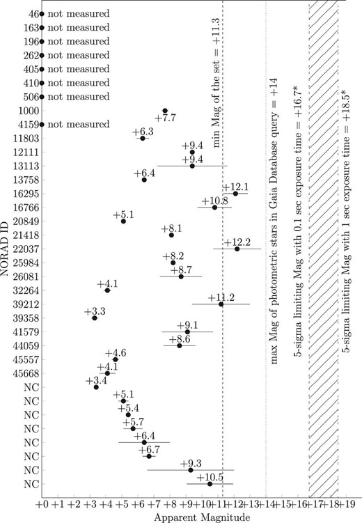
Photometry of 35 objects detected. NC are non-cataloged objects. Eight objects were not measured as one of their ends was out of bounds of the image sensor. The dashed vertical line indicates the minimum detectable apparent magnitude of the set, which is +11.3. The dotted vertical line indicates the limiting magnitude of reference stars in the query to the Gaia database, which is +14. The area with the diagonal pattern encompasses the 5σ limiting magnitudes between 0.1 (+16.7) and 1 s (+18.5) exposure time. Horizontal bars in each coordinate represent the error in the calculation of the apparent magnitude, which is the magnitude residual value in each result. “*” means the specifications from Sako et al. (2018).
The minimum detectable apparent magnitude, considering the residual error, is + 11.3, which is the lowest value that corresponds to the object with NORAD ID 16295, so we consider this value as the sensitivity of the system.
Concerning processing time, figure 8 shows the results of a comparison in the detection stage when processing with a GPU and a CPU. Figure 9 shows the results with a CPU, 1 × GPU, and 4 × GPU (our system), considering the entire pipeline processing time, including preprocessing, detection, and postprocessing (astrometry + identification) for two different thresholds.
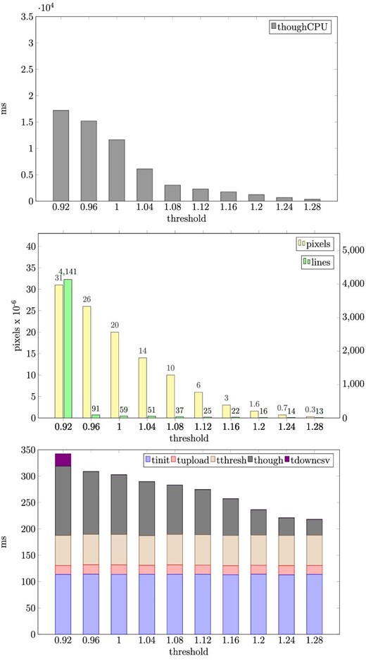
Comparison of CPU vs. GPU processing times in the detection stage for a range of thresholds. (Top) Processing time of the PPHT algorithm in the CPU. (Center) Number of pixels to process and number of lines detected for each threshold. (Bottom) Processing time of all steps of the detection stage in the GPU.
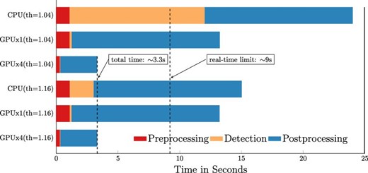
Comparison of CPU vs. GPU processing times in the total processing pipeline for two thresholds (low sensitivity, th = 1.16; high sensitivity, th = 1.04).
Figure 8 (top) shows the PPHT step of the detection stage when one FITS image file is processed using the CPU. In this case, the other steps of the detection stage are not represented in this figure, as their contribution is much smaller than the PPHT processing time, which accounts for most of the detection stage processing time. The threshold represents the factor to multiply by the mean value of the image, to binarize it before the PPHT is applied. This value defines the sensitivity of the detection stage. When this value is high (th = 1.28), the number of pixels to process is low, so the process is fast though less sensitive, and when this value is low (th = 0.92), the number of pixels to process is high, but the process is more sensitive, as we are close to the background noise of the image. Figure 8 (center) shows the number of pixels to process, and the number of lines detected as the threshold changes. Figure 8 (bottom) shows the processing time of the detection stage, when one GPU is used, including all steps of this stage. Note that the vertical scale of figure 8 (top) is 100 times that of figure 8 (bottom). Comparing the top and bottom parts of figure 8, we see that the GPU is much faster than the CPU in the PPHT stage for all sensitivity values, and this difference is greatly accentuated when the threshold is low. In the GPU, all steps of the detection stage show a consistent time, with not much change in the timing. These results show that the PPHT process in the GPU is ∼130 times faster than in the CPU for a high sensitivity threshold (th = 0.92), and ∼12 times faster for a low sensitivity threshold (th = 1.28).
Figure 9 compares the CPU/GPU×1/GPU×4 of the whole processing pipeline applied to one FITS image file of the set with two different thresholds, 1.16 (lower sensitivity) and 1.04 (higher sensitivity). Most of the postprocessing time (blue bar) is used by the identification process because the algorithm needs to compare each of the detected streak ends with a large database of 29084 objects downloaded from the space-track.org public database; in the worst case, it can take up to ∼12 s (the case shown in figure 9). The real-time target for this experiment is 9 s because each FITS file is composed of 18 consecutive frames of 0.5 s exposure time. From figure 9, we can see that the CPU never reaches the real-time target, even for a low sensitivity threshold. For high sensitivity (th = 1.04), the CPU cannot reach the real-time target due to the long processing time of the PPHT stage. With one GPU, the preprocessing and detection stage times are well below the target time due to the dramatic reduction in the long processing time in the PPHT stage, but the long processing time due to the postprocessing stage still takes longer than the real-time target. Nevertheless, if we use the proposed method with four parallel GPU threads, all these times are divided by four, and we can easily comply with the real-time target proposed in this experiment. However, it is important to note that in a normal scenario, when processing a large batch of FITS image files, statistically, we detect streaks in only a few of them, and the postprocessing stage starts only when streaks are detected, so normally, we would reach the real-time target with fewer than four GPUs.
8 Conclusions
Our study has developed a fast algorithm implemented in a four-CPU–GPU system to detect streaks in astronomical images in real time (faster than images are produced), which is particularly useful when there is a massive amount of image data or when data need to be transferred from one observation site to the next quickly to follow up objects. We tested the system with two hours of observation data (20084 FITS files) from the Tomo-e Gozen camera of the 1M telescope at Kiso Observatory (Japan). We achieved the real-time target with the system (3.3 s out of 9 s). The streaks detected were in the 350 (all elevations) to 2000 km (from 35° elevation and higher) altitudes in LEO. The minimum detectable streak had an apparent magnitude of +11.3 in the Gaia G band. From the dataset, streaks were detected in 0.5% of the images, and 27 out of 35 streaks were identified as real objects when compared to a database of 29082 TLE-based records from space-track.org. This system can help establish optical observations as a reliable and sensitive tool to track existing space debris and other objects in LEO and detect new ones in real time, so data handover between observation stations is facilitated. This processing pipeline also drastically cuts processing time when a massive volume of image data needs to be processed to find space debris or track objects. These two features make this processing pipeline a useful technique for addressing the increasingly critical issue of space debris.
Acknowledgments
Astronomical images files were provided by the Tomo-e Gozen Team of the University of Tokyo. This research made use of Photutils, an Astropy package for detection and photometry of astronomical sources.3
Footnotes
P. V. C. Hough 1962, US Patent 3069654.
L. Bradley, et al. 2021, astropy/photutils: v.1.1.0, Zenodo 〈https://doi.org/10.5281/zenodo.4624996〉.
References
Author notes
JSPS International Research Fellow (JAXA).
