


Abstract
We derive the entire dust extinction (AV) map for the Large Magellanic Cloud (LMC) estimated from the color excess at near-infrared wavelengths. Using the percentile method we recently adopted to evaluate AV distribution along the line of sight, we derive three-dimensional (3D) AV maps of the three massive star-forming regions of N44, N79, and N11 based on the IRSF/SIRIUS point source catalog. The 3D AV maps are compared with the hydrogen column densities N(H) of three different velocity components where one is of the LMC disk velocity and the other two are of velocities lower than the disk velocity. As a result, we obtain a 3D dust geometry suggesting that gas collision is ongoing between the different velocity components. We also find differences in the timing of the gas collision between the massive star-forming regions, which indicates that the gas collision in N44, N79, and N11 occurred later than that in 30 Doradus. In addition, a difference of a factor of two in AV/N(H) is found between the velocity components for N44, while a significant difference is not found for N79 and N11. From the 3D geometry and AV/N(H) in each star-forming region, we suggest that the massive star formation in N44 was induced by an external trigger of tidal interaction between the LMC and the Small Magellanic Cloud, while that in N79 and N11 is likely to have been induced by internal triggers such as gas converging from the galactic spiral arm and expansion of a supershell, although the possibility of tidal interaction cannot be ruled out.
1 Introduction
The Large Magellanic Cloud (LMC) is a dwarf galaxy with morphological features such as an off-center stellar bar and a single spiral arm, accompanied by the Magellanic Bridge, which is a H i gas structure connecting the LMC and the Small Magellanic Cloud (SMC). These features are considered to be evidence for the tidal interaction between the LMC and the SMC (e.g., Besla et al. 2012; Diaz & Bekki 2012). The LMC is one of the nearest interacting galaxies at a distance of ≃50
Recent studies using H i and CO data suggest that the massive star formations in 30 Dor and N159 in the LMC H i ridge region were induced by the galactic interaction between the LMC and the SMC (Fukui et al. 2017, 2019; Tokuda et al. 2019). Fukui et al. (2017) identify two velocity H i components; one is the velocity component of the LMC disk and the other is a low-velocity component relative to the disk velocity. Fukui et al. (2017) and Tsuge et al. (2019) identify an intermediate-velocity component between them for 30 Dor and N159, which is considered to be evidence for gas collision. In addition, they evaluate the dust/gas ratio from the comparison of the H i intensity with the dust optical depth, and find that the dust/gas ratio for the LMC H i ridge region is lower than that for the LMC stellar-bar region. Based on the low dust/gas ratio and numerical simulations (e.g., Bekki & Chiba 2007a, 2007b; Yozin & Bekki 2014), they suggest that low-metallicity gas from the SMC (Z ∼ 0.2 Z⊙; Russell & Dopita 1992) is falling on to the LMC disk. More recently, Tsuge et al. (2020) investigated the spatial correlation between the intermediate-velocity component and massive stars in the entire LMC field, and suggest that the galactic interaction may have induced a large part (∼70%) of the massive star formation in the LMC. In order to investigate such gas collisions between the gas in the LMC and an inflow gas from the SMC, it is important to study the dust/gas ratio and three-dimensional (3D) dust geometry over the whole LMC.
Furuta et al. (2019) constructed a near-infrared (NIR) dust extinction (AV) map of the LMC H i ridge region to evaluate the dust/gas ratio. They proposed a method to decompose AV into different velocity components from the comparison of AV with hydrogen column densities of different velocities. They decomposed AV into the three velocity components mentioned above, and found that the dust/gas ratio of the low-velocity component is significantly lower than that of the disk-velocity one. Furthermore, Furuta et al. (2021) developed a new method to evaluate 3D dust geometry from the NIR dust extinction, and applied it to the H i ridge region. They decomposed the resultant 3D AV map into the three velocity components using the fitting method described in Furuta et al. (2019), and obtained the detailed dust geometry of the different velocity components, from which they found that the gas collision with the inflow gas from the SMC had occurred in 30 Dor prior to N159.
In the present paper, we extend the analysis of the LMC H i ridge region by Furuta et al. (2021) to the entire LMC field. We especially focus on the massive star-forming regions of N44, N79, and N11 for which the tidal interaction between the Magellanic Clouds is reported (Tsuge et al. 2019, 2020). This paper is organized as follows: we summarize the data in section 2 and give a brief review of the method to evaluate the 3D dust extinction in section 3. The resultant dust extinction maps and a comparison with gas observations are presented in section 4. We discuss the 3D geometry and origin of massive star-forming regions in section 5, and summarize our results in section 6.
2 The data
2.1 Point source catalog observed with IRSF/SIRIUS
We used the NIR (J, H, and Ks bands) Magellanic Cloud point source catalog observed with the InfraRed Survey Facility (IRSF) 1.4 m telescope (Kato et al. 2007; hereafter the IRSF catalog). The IRSF catalog covers a 40
Since Galactic foreground stars leading to underestimation of the dust extinction are included in the IRSF catalog, we identify stellar populations using the classification by Furuta et al. (2019). Stellar populations are classified into three categories that primarily consist of Galactic foreground contamination, red giant branch (RGB) stars, and dwarf stars, using a color–magnitude (J − K vs. K) diagram (figure 1a). In the present paper, only the objects classified as RGB stars are used, a number density map of which is shown in figure 2.
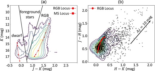
(a) Color–magnitude (J − K and K) diagram of the samples of the entire LMC. Contours show the number densities binned by 0.05 mag. The contour levels are 101.5–103.5 in steps of 100.5. Black solid lines are boundary positions to classify stellar populations into three categories of dwarf, foreground, and RGB stars. The lines connected with the circles and squares are the loci of RGB and main-sequence stars, respectively, derived from Allen (2000). (b) Color–color (H − K and J − H) diagram of the RGB samples selected from panel (a). Contours are the same as those in panel (a) but the levels are 101.5–104.5 in steps of 100.5. The line connected with the red circles shows the intrinsic colors of RGB stars derived from Bessell and Brett (1988). The black arrow is the reddening vector corresponding to AV = 10 mag. Black points are YSO candidates matched to the RGB samples. (Color online)
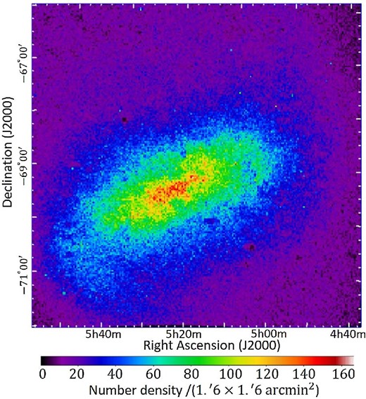
RGB star number density map of the LMC. The grid size is
In principle, intrinsically red stars such as young stellar objects (YSOs) can contaminate the selected RGB samples. To check the contamination of YSOs, we match the RGB samples with the YSO candidates in the whole LMC derived from Whitney et al. (2008), Gruendl and Chu (2009), and Seale et al. (2014). We also use the list of YSOs presented by Carlson et al. (2012), who identify YSOs in the nine star-forming regions in the LMC. The total number of YSO candidates is 5714. A matching distance of
2.2 Gas tracer
For comparison of the dust extinction with the hydrogen column density, we use the H i data observed with the Australia Telescope Compact Array (ATCA) and Parkes (Kim et al. 2003), and the 12CO (J = 1–0) data observed with the NANTEN 4
2.3 Dust emission
To compare the dust extinction with the dust emission, we use the dust optical depth at 353 GHz (τ353) derived from the Planck and IRAS data (Planck Collaboration 2014). The comparison between the dust extinction and emission gives an insight into the dust geometry because the dust extinction only traces the dust located in front of stars, while the dust emission traces all the dust existing along the line of sight. As a dust emission map of the LMC, we use the τ353 map created by Tsuge et al. (2019), who subtract the Galactic foreground τ353 values. The spatial resolution of the τ353 map is adjusted to that of the dust extinction map by the same procedure as the gas maps.
3 Method
Furuta et al. (2021) developed a new method to evaluate the 3D dust geometry for study of the LMC H i ridge region. The detailed procedure is described in their paper (see section 3 of Furuta et al. 2021). Here, we introduce a brief review of the method.
3.1 Derivation of dust distribution along the line of sight
Below we show the calculation procedure of dust distribution along the line of sight for a low H i column density region (
Procedure to estimate AV along the line of sight in a spatial bin of
Here, it is noted that recent studies show the dependence of RGB colors on stellar metallicity (e.g., Valenti et al. 2004) together with the metallicity gradient in the LMC (e.g., Choudhury et al. 2021), which can lead to an unintended bias in AV at different galactocentric distances across the LMC with the intrinsic colors of Bessell and Brett (1988) that do not consider the metallicity dependence. Therefore, we check how much the intrinsic colors are affected by the metallicity gradient. Choudhury et al. (2021) find the average metallicity of [Fe/H] = −0.42 dex and a shallow metallicity gradient of −0.008 dex
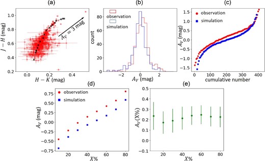
In the second step, we sort the estimated AV from low to high for each spatial bin. The sorted AV distribution is shown by the red histogram in figure 3b, while the sorted AV values at every five stars are shown by the red circles as a function of the cumulative number of stars in figure 3c. The AV values in figure 3c monotonically increase due to the dust existing along the line of sight. However, even when no dust exists along the line of sight, the sorted AV values increase due to the AV scatter caused by the photometric errors. Thus, in the third step, we simulate the AV scatter by a Monte Carlo simulation to evaluate this effect.
We generate a random set of the J − H and H − K colors for individual stars on the CC diagram in each spatial bin under the assumption that the stellar colors follow a 2D Gaussian distribution. Here, we adopt the observed colors and photometric errors as the center and the standard deviation of the Gaussian distribution, respectively. AV for each simulated star is calculated by the same procedure as the first step. The blue histogram and squares in figures 3b and 3c, respectively, show the resultant distribution of the simulated values, which is considered to be AV scatter due to the photometric errors alone.
In the next step, the mean percentile values for both observed and simulated AV are calculated in the range of the X% to (X + 10)% percentile for X = 10% to 80% in steps of 10%. Here, we adopt not
The uncertainty of AV(X%) is measured by the error propagation,
AV(X%) in figure 3e is almost constant for all X%, which indicates that dust clouds associated with the LMC are not detected significantly at this spatial bin, as expected from the low column density region. The constant AV of 0.2 mag is likely to be caused by the Galactic foreground extinction and is actually consistent with the foreground extinction ∼0.2 mag (Dobashi et al. 2008).
In figure 4, we present another result for the spatial bin centered at (α, δ)J2000.0 = (
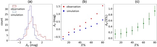
Same as panels (b), (d), and (e) of figure 3 but for the region having a high column density of the D-component at (α, δ)J2000.0 = (
![Total integrated dust extinction map [$A_V(80\%)$] in the entire LMC field. The spatial resolution is ${5^{\prime }}$ with a grid size of ${1{^{\prime }_{.}}6}$. Black contours show the total hydrogen column density covering all the velocity ranges of the L-, I-, and D-components with contour levels of $(2.0\mbox{--}8.0) \times 10^{21}\, \rm cm^{-2}$ in steps of $2.0\times 10^{21}\, \rm cm^{-2}$. White contours show the total hydrogen column density of the L-component with levels of $(0.7,\ 1.6,\ 2.5,\ 3.4,\ 4.2,\ 5.1,\ \mbox{and}\ 6.0) \times 10^{21}\, \rm cm^{-2}$. Gray regions are masked bins due to the inappropriate observational data. (Color online)](https://oup.silverchair-cdn.com/oup/backfile/Content_public/Journal/pasj/74/3/10.1093_pasj_psac025/3/m_psac025fig5.jpeg?Expires=1749356717&Signature=vWuGTues~6kQq0Leh4qSh-DLPP2jGCnZ5B0eposiIoRusIDTDd4y7mt-O62eS~ywakttNzdpcTo4KkEXwuBW2wIBFrV7CldGz8HZu5j~nP7jvv7RzFTZRSxEVhMf8bQubWl6RCbh8a4zUB-vXU1BfJeHRLAKWywzw2xTUOA-eZrcqGbOfnmNv-RuarPk5L5Gg4wiYHmoVL4RZZtmg6rVl-59MJ8PpZi-1E4wxVgW1PcH54Xl9Fo-tj0BitkrUDtRayh4qc9wGLMhPYzVmaNPC9hSysKCMVttNVoWI8r9yZj7giULxDxavIQCsc~hFy7AaCw--EnIDDIfMfsl~1h1BA__&Key-Pair-Id=APKAIE5G5CRDK6RD3PGA)
Total integrated dust extinction map [
![Uncertainty map [$\delta A_V(80\%)$] of the total integrated dust extinction map in figure 5. White contours are the same as the black contours in figure 5. (Color online)](https://oup.silverchair-cdn.com/oup/backfile/Content_public/Journal/pasj/74/3/10.1093_pasj_psac025/3/m_psac025fig6.jpeg?Expires=1749356717&Signature=Tc7dUFaRuP6XVEPCM2EULUqu-gw08Xflxo3xyEKlVsvp45jxufG9gFDT-AxTv7AQYh2dlcnbwUJcb7m8HMAvtWxnIUg8GbGMdJ6QG~WtZXx-EEMTZ0HvcT3z72HJxqjUEZW9jE2gu3N8hlNU4OCuGtY0OgnUGGDxbo61~HLz83u67GkuyQTvMcOeAhhIGSRpY-eG6xh3gS8S2MyUq92hzItjIlizXgR2KNsi5Jp~9gwMcbZ2tzo6aiqy0HXKeh0XIQb5qjYFAvyuI7xG1djjQZ2nDcTApKtvTg44nKgSo3Ekv6jc5iqJeoaBfIAzNlGUylMlXJy69e0Pxagr4bf2YQ__&Key-Pair-Id=APKAIE5G5CRDK6RD3PGA)

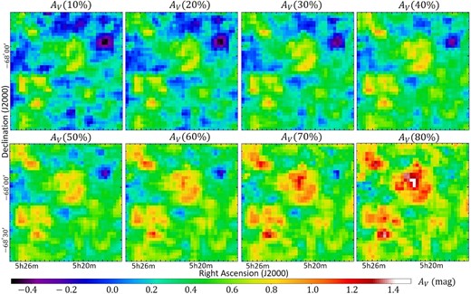
Integrated dust extinction maps of N44 from observers to stars included in the
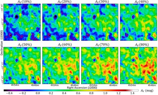
Same as figure 8 but for N79. (Color online)
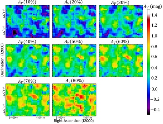
Same as figure 8 but for N11. (Color online)
3.2 Decomposition of dust extinction into different velocities
Same as figure 11 but for N79. Contour levels are also the same as those in figure 11. The comparison of
Same as figure 11 but for N11. Contour levels are also the same as those in figure 11. The comparison of
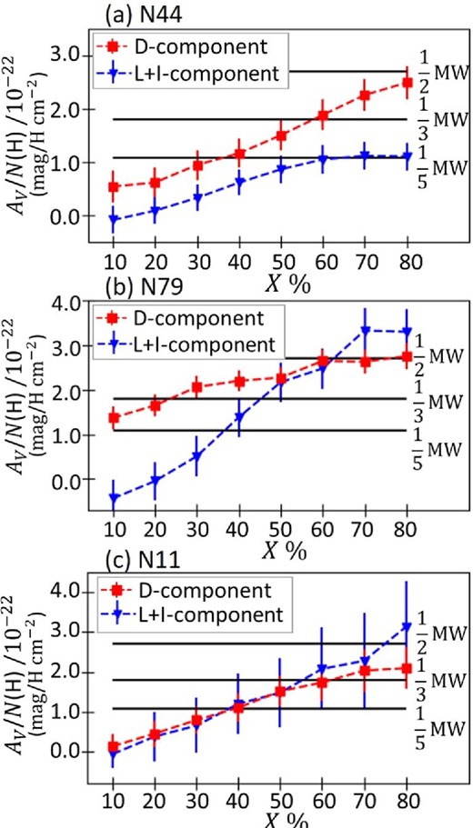
Fitting parameters of AV/N(H) for (a) N44, (b) N79, and (c) N11 estimated from the linear regression of equation (2). Squares and triangles are the parameters of the D- and L+I-components, respectively. Black horizontal lines are 1/5, 1/3, and 1/2 of AV/N(H) in the Milky Way (MW). (Color online)
4 Result
4.1 Cumulative dust extinction map over the LMC
In figure 5, we show the AV(80%) map (i.e., near-total integrated dust extinction map) of the entire LMC field. The spatial resolution of the map is
We compare the AV(80%) map with the dust extinction map created by Dobashi et al. (2008) using the 2MASS catalog in figure 7. The spatial distribution of high AV regions such as the H i ridge region and N44 is consistent between the AV maps in figures 5 and 7. The AV(80%) map significantly detects dust clouds in N79 and around (α, δ)J2000.0 = (
In figure 5, we recognize that the dust extinction correlates well with the total hydrogen column density. Relatively high AV regions (AV > 1.0 mag) can be seen in the massive star-forming regions of the H i ridge, N44, N79, and N11. On the other hand, in the region where Tsuge et al. (2020) identify the diffuse L-component (hereafter the diffuse L-com region), no dust cloud is detected.
4.2 Cumulative dust extinction toward individual star-forming regions
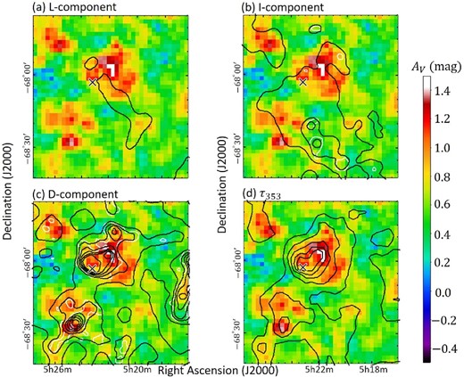
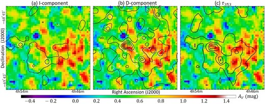
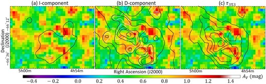
In this section, to evaluate the 3D dust geometry and the dust/gas ratio of different velocity components in the massive star-forming regions of N44, N79, and N11, we investigate spatial correlation between AV and N(H) of different velocities. Figures 8–10 show the AV(10%) to AV(80%) maps of N44, N79, and N11, respectively. Since these maps show the dust extinction integrated from observers to X%, the dust extinction should increase with X%. We also present a comparison of AV(80%) with N(H) of different velocity components and dust emission of τ353 for N44, N79, and N11 in figures 11–13, respectively.
The analysis area of each star-forming region shown in figures 8–10 is determined based on the areas for which Tsuge et al. (2019, 2020) investigate the spatial and velocity distributions of the H i clouds. Although they are larger than the H ii regions of N44, N79, and N11 defined in the Henize (1956) catalog, we adopt these analysis areas covering the L- and/or I-components existing around each
star-forming region to investigate the 3D dust geometry of different velocity components.
4.2.1 N44
From figure 11, we recognize that the dust extinction exhibits a good spatial correlation with N(H) of the D-component and τ353, which indicates that all the dust clouds in N44 are located in the LMC disk. On the other hand, we cannot see a clear spatial correlation between the dust extinction and the L- and I-components.
In order to statistically determine whether the AV counterparts of the L- and/or I-components are detected in the AV(80%) map, we apply the fitting with equation (2) to the AV(80%) map. Since N(H) of the L-component is low for a large area as shown in figure 11a, to improve the statistics, we newly define the L+I-component whose velocity range is −100 to −10
To check the validity of introducing the L+I-component, we separate the L+I-component into the L- and I-components and perform the fitting with equation (2) using k = D, L, and I with the same XCO factor for the D-, L-, and I-components (i.e., xD = xL = xI). As a result, χ2
To evaluate the 3D geometry of N44, we apply the fitting with equation (2) using the D- and L+I-components to each AV(X%) map for X = 10% to 80%. Table 1 shows the best-fitting parameters, while figure 14a shows AV/N(H) of the L+I- and D-components thus obtained as a function of X%. The uncertainties of the parameters are calculated by formal regression errors using the AV uncertainties of
Fitting parameters estimated from the comparison of AV with
| ak | xD (XCO)* | ||||
|---|---|---|---|---|---|
| Name | Percentile | Reduced χ2 | L+I-component | D-component | D-component |
| N44 | AV(10%) | 0.36 | −0.09 ± 0.26 | 0.54 ± 0.30 | 3.0 ± 4.6 |
| AV(20%) | 0.64 | 0.09 ± 0.25 | 0.62 ± 0.28 | 2.5 ± 3.7 | |
| AV(30%) | 0.85 | 0.33 ± 0.25 | 0.95 ± 0.28 | 1.0 ± 2.0 | |
| AV(40%) | 1.01 | 0.61 ± 0.24 | 1.16 ± 0.27 | 0.9 ± 1.6 | |
| AV(50%) | 1.11 | 0.86 ± 0.25 | 1.50 ± 0.28 | 0.3 ± 1.2 | |
| AV(60%) | 1.09 | 1.05 ± 0.26 | 1.88 ± 0.29 | −0.3 ± 1.0 | |
| AV(70%) | 0.89 | 1.12 ± 0.26 | 2.26 ± 0.30 | 0.2 ± 1.0 | |
| AV(80%) | 0.46 | 1.11 ± 0.26 | 2.49 ± 0.30 | 1.5 ± 1.0 | |
| N79 | AV(10%) | 0.30 | −0.43 ± 0.43 | 1.37 ± 0.25 | 0.7 ± 1.9 |
| AV(20%) | 0.60 | −0.05 ± 0.43 | 1.65 ± 0.25 | 1.3 ± 1.6 | |
| AV(30%) | 0.84 | 0.51 ± 0.45 | 2.06 ± 0.25 | 0.2 ± 1.2 | |
| AV(40%) | 1.01 | 1.38 ± 0.44 | 2.20 ± 0.24 | 0.6 ± 1.1 | |
| AV(50%) | 1.22 | 2.17 ± 0.43 | 2.27 ± 0.24 | 1.9 ± 1.2 | |
| AV(60%) | 1.34 | 2.48 ± 0.46 | 2.64 ± 0.25 | 2.0 ± 1.1 | |
| AV(70%) | 1.26 | 3.33 ± 0.50 | 2.62 ± 0.26 | 1.9 ± 1.1 | |
| AV(80%) | 0.71 | 3.30 ± 0.51 | 2.75 ± 0.28 | 2.9 ± 1.3 | |
| N11 | AV(10%) | 0.17 | −0.06 ± 0.35 | 0.14 ± 0.31 | 40.3 ± 112.6 |
| AV(20%) | 0.39 | 0.40 ± 0.63 | 0.45 ± 0.33 | 5.1 ± 11.0 | |
| AV(30%) | 0.60 | 0.65 ± 0.69 | 0.79 ± 0.34 | 3.5 ± 6.0 | |
| AV(40%) | 0.73 | 1.20 ± 0.76 | 1.10 ± 0.36 | 0.8 ± 4.1 | |
| AV(50%) | 0.99 | 1.48 ± 0.87 | 1.51 ± 0.38 | −0.8 ± 3.0 | |
| AV(60%) | 1.14 | 2.08 ± 1.03 | 1.73 ± 0.46 | −1.1 ± 2.9 | |
| AV(70%) | 1.09 | 2.28 ± 1.19 | 2.03 ± 0.54 | −0.1 ± 3.3 | |
| AV(80%) | 0.42 | 3.13 ± 1.14 | 2.09 ± 0.53 | 2.8 ± 3.3 | |
The units are
In table 1, many of the derived XCO factors of N44 for X = 10%–80% are not estimated significantly (i.e., XCO < 1σ, where σ is the uncertainty of XCO). This result indicates that AV counterparts of CO molecules are not detected in many of our AV maps. Actually, in the total integrated AV map [AV(80%)], the XCO factor is estimated significantly (XCO > 1σ). From table 1, we find that the AV/N(H) ratio at X = 80% for the L+I-component of N44 is lower than that for the D-component. Since XCO is known to depend on the metallicty (Bolatto et al. 2013), we need to check the validity of using the same XCO factor for the L+I and D-components in the fitting. Hence, by tentatively setting XCO for the L+I-component as a new free parameter independent of the D-component, χ2
4.2.2 N79
In figure 12b, the D-component gas correlates well with the dust extinction map, although the right-hand side of the map is noisy due to the low number densities of the stars (figure 2). Dust emission τ353 also shows the spatial correlation with the dust extinction, indicating that all the dust is present in the LMC disk.
To check whether the AV counterparts of the I-component are detected significantly, we apply the same fitting procedure for N44 to the AV(80%) map of N79. By adding the L+I-component to the fitting with the D-component alone, χ2
From table 1, we find that XCO for N79 is not detected significantly at
4.2.3 N11
From figures 13a and 13b, we recognize that dust clouds are detected in the regions where the D- and I-components are detected. In fact, by adding the L+I-component to the fitting with the D-component alone, χ2/dof is improved from 37.07
From table 1, we recognize that the AV/N(H) ratio at
4.3 Dust geometry for the diffuse L-com region
In the “diffuse L-com region” that is located in the west of N44 and marked in figure 5, Tsuge et al. (2020) find that there is no significant H ii region in the area where the L-component exists. They also find that there is no signature of deceleration of the L-component in the first moment map of the diffuse L-com region, and thus they suggest that the L-component in this region is located behind the LMC disk, and the gas collision is yet to occur. To verify this hypothesis, we evaluate the 3D geometry of this region.
In figure 15, we show the AV(80%) maps with N(H) of the L-, I-, and D-components and τ353. In figure 15a, we cannot see a clear spatial correlation between the L-component and the dust extinction. The D-component extends in this region and roughly correlates with the dust extinction in figure 15c, while the CO emission of the D-component (shown by white contours in figure 15c) does not correlate with the dust extinction, especially in the south of the map, which indicates that the molecular gas is located on the far side of the LMC disk.

To determine whether the AV counterparts of the L- and/or I-components are detected significantly, we apply the linear regression fitting to the AV(80%) map similarly to N44. Since the AV counterparts of molecular gas are not detected as mentioned above, we mask the regions in the AV map where the CO intensity is higher than 1.5σ and perform the fitting with equation (2) using only the H i data. By adding the L+I-component to the fitting with the D-component alone, χ2
To evaluate the geometry of the I- and D-components, we apply the fitting with equation (2) using N(H i) of the I- and D-components to each AV(X%) map. The estimated parameters of AV/N(H) are summarized in table 2 and shown in figure 16. AV/N(H) of the D-component monotonically increases with X%, indicating that the dust of the D-component extends along the line of sight. The AV/N(H) ratio of the I-component agrees with that of the D-component. Thus, the dust of the I-component is likely to be distributed similarly to that of the D-component. In summary, in the diffuse L-com region, the L-component is located behind the LMC disk, while the I- and D-components extend along the line of sight, which is consistent with the hypothesis that gas collision is yet to occur, as mentioned by Tsuge et al. (2020).
Same as table 1 but for the diffuse L-com region.
| I-component | D-component | ||
|---|---|---|---|
| Name | Reduced χ2 | aI | aD |
| AV(10%) | 0.51 | 0.27 ± 0.59 | −0.30 ± 0.36 |
| AV(20%) | 1.00 | −0.01 ± 0.59 | 0.52 ± 0.37 |
| AV(30%) | 1.39 | 0.34 ± 0.57 | 1.20 ± 0.35 |
| AV(40%) | 1.65 | 0.93 ± 0.56 | 1.67 ± 0.35 |
| AV(50%) | 1.81 | 1.71 ± 0.56 | 2.07 ± 0.35 |
| AV(60%) | 1.98 | 2.19 ± 0.59 | 2.59 ± 0.37 |
| AV(70%) | 1.69 | 2.62 ± 0.62 | 2.79 ± 0.37 |
| AV(80%) | 1.07 | 2.89 ± 0.61 | 2.77 ± 0.38 |
The units are 10−22 mag/(H
5 Discussion
5.1 Dust geometry of individual star-forming regions
In this section, we evaluate the dust geometry of N44, N79, and N11 from the estimated fitting parameter of ak [i.e., AV/N(H)] of each X%. We first consider the dust geometry of N44. The likely 3D dust geometry of the D- and L+I-components for N44 is illustrated in figure 17a. First, AV/N(H) of the D-component in figure 14a monotonically increases with X%, and thus the D-component is expected to extend along the line of sight as shown by a red rectangle in figure 17a, which is consistent with the general idea that the gas of the LMC disk is mixed with stars. AV/N(H) of the L+I-component is significantly detected from X = 30% onward, which indicates that the head of the L+I-component is located at X = 30%. In addition, AV/N(H) of the L+I-component is almost constant from X = 60% to 80%, indicating that there is little dust of the L+I-component beyond X = 60%. As a whole, the L+I-component in N44 is likely to extend from X = 30% to 60% as shown by a blue rectangle in figure 17a. The dust geometry suggests that the L+I-component is penetrating the D-component. This trend supports the idea that gas collision between the gas of the LMC disk and an inflow gas as seen in the L+I-component may have induced the massive star formation in N44 (Tsuge et al. 2019).

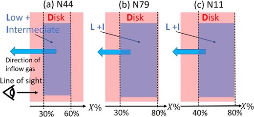
Side view of the expected dust geometry of (a) N44, (b) N79, and (c) N11. Red and blue rectangles denote the disk-velocity component (D-component) and the low+intermediate-velocity component (L+I-component), respectively. (Color online)
Similarly to N44, we discuss the 3D dust geometry of N79 and N11. In both regions, from the monotonic increase of AV/N(H) of the D-component with X% in figures 14b and 14c, the D-component is expected to extend along the line of sight as shown by red rectangles in figures 17b and 17c. AV/N(H) of the L+I-component is not detected significantly at X = 10%–20% and X =10%–30% for N79 and N11, respectively (see table 1), and thus the L+I-component is expected to extend beyond X = 30% for N79 and beyond X = 40% for N11 as shown by blue rectangles in figures 17b and 17c, respectively.
We compare the dust geometry of N44, N79, and N11 as well as the H i ridge region with the evolutionary stages of giant molecular clouds (GMCs) proposed by Kawamura et al. (2009). We summarize the positions of the L- or L+I-components and evolutionary stages of the relevant GMCs in table 3. The H i ridge region is separated into three regions based on the geometry of the L-component by Furuta et al. (2021). They define them as regions 1–3 from north to south; regions 1 and 2 contain 30 Dor and N159, respectively (see figure 14 in Furuta et al. 2021). The evolutionary stages are classified into four stages, Types I–III and the last stage in order from youngest to oldest. From the positions relative to the LMC disk of the L+I-component for N44, N79, and N11 in table 3, we recognize that the gas collision in these regions occurred later than in 30 Dor but occurred earlier than in region 3, which is consistent with the evolutionary sequences of the GMCs. The evolutionary stage of GMCs in N79 is earlier than those of N159, N44, and N11. However, we cannot see clear differences in the timing of gas collisions between these regions. This is likely to be caused by the large AV uncertainties, especially for N79 and N11, due to the low number densities of the stars.
Comparison of dust geometry of the L- or L+I-component with evolutionary stages of the related giant molecular clouds.
| Position | Evolutionary | |
|---|---|---|
| Name | (L- or L+I-component) | stage* |
| 30 Dor (region 1 in H i ridge) | front of the disk† | last stage |
| N159 (region 2 in H i ridge) | X = 30% to 80%† | Type III |
| region 3 in H i ridge | behind the disk† | Type I |
| N44 | X = 30% to 60% | Type III |
| N79 | X = 30% to 80% | Type II |
| N11 | X = 40% to 80% | Type III |
In order to discuss the relationship between the timing of the gas collision and the evolutionary stages of GMCs quantitatively, we compare the crossing timescale of the gas collision with the transition timescale of the evolutionary stages. For example, from the comparison of the dust geometry of 30 Dor with that of N44, the head of the L+I-component is separated by the distance of the 30% percentile. Considering am LMC disk thickness of 2 kpc (Balbinot et al. 2015), this corresponds to 0.6 kpc. Assuming the velocity of the inflow gas (L-component) to be ∼100 km s−1 (Tsuge et al. 2020), it takes 6 Myr for the inflow gas to cross 0.6 kpc, which is consistent with the timescale of 7 Myr for the transition from Type III GMCs in N44 to the last-stage GMCs in 30 Dor (Kawamura et al. 2009). Therefore, our result can reasonably explain the difference in the evolutionary stages of the GMCs across the LMC.
5.2 Origin of massive star-forming regions
We discuss the origins of the massive star-forming regions of N44, N79, and N11 from the AV/N(H) ratio at
AV/N(H) and XCO at
| L or L+I-component | I-component | D-component | ||
|---|---|---|---|---|
| Name | aL | aI | aD | xD (XCO)† |
| H i ridge | 1.24 ± 0.13‡ | 1.36 ± 0.17‡ | 2.08 ± 0.14‡ | 1.7 ± 1.0‡ |
| N44 | 1.11 ± 0.26 | — | 2.49 ± 0.30 | 1.5 ± 1.0 |
| N79 | 3.30 ± 0.51 | — | 2.75 ± 0.28 | 2.9 ± 1.3 |
| N11 | 3.13 ± 1.14 | — | 2.09 ± 0.53 | 2.8 ± 3.3 |
The AV/N(H) ratio of the D-component at X =80% for the star-forming regions of N44, N79, and N11 is similar to that of the H i ridge region (see table 4). The resultant AV/N(H) ratio is nearly half of that in the Milky Way
On the other hand, AV/N(H) of the L+I-component significantly varies between the star-forming regions. For N44, AV/N(H) of the L+I-component is ∼1/5 of the Galactic value, which is similar to the dust/gas ratio for the SMC of ∼1/6 of the Galactic value (Roman-Duval et al. 2014). The existence of low-metallicity gas in the L+I-component in N44 supports the contamination of the inflow gas from the SMC, as proposed by Tsuge et al. (2019).
In N44, expansion of H i shell is reported (Kim et al. 1998). Around the shell, three episodes of massive star formation are found; one is the ∼10 Myr-old star formation inside the shell, another is the ∼5 Myr-old star formation on the shell rims, and the other is the YSOs (typically <1 Myr-old) (e.g., Oey & Massey 1995; Chen et al. 2009; Carlson et al. 2012). Tsuge et al. (2019) propose that the 5 Myr-old massive star formation was triggered by the galactic interaction between the LMC and the SMC as an alternative scenario of star formation triggered by the expansion of the H i shell from the existence of low-metallicity gas and signature of gas collision between the L- and I-components in addition to the lack of energy supply from the shell to explain the motions of the L-, I-, and D-components in N44. The age of the stellar population of N44 (∼5 Myr) is younger than that around the 30 Dor region of 8.1 Myr (Schneider et al. 2018), which agrees with the difference in the evolutionary stages of GMCs between N44 and 30 Dor (see table 3). Therefore, from the low AV/N(H) ratio of the L-component and the gas-colliding geometry in figure 17a, we suggest that the massive star formation around the shell rims in N44 was triggered by the galactic interaction between the Magellanic Clouds, similarly to the H i ridge region.
For N79 and N11, AV/N(H) of the L+I-component at X = 80% is nearly half of the Galactic value, which is similar to that of the D-component. According to the recent numerical simulations of the tidal interaction between the LMC and SMC (Tsuge et al. 2020), the gas currently falling on to the LMC disk as the L+I-component consists of gas from the LMC as well as from the SMC. We thus expect that in some places the metallicity will not be very different from that of the LMC, if the L+I-component is dominated locally by the LMC gas. In addition, an analysis of the dust/gas ratio based on the Planck dust emission of τ353 (K. Tsuge et al. in preparation ) indicates that the dust/gas ratio toward N79 and N11 is about two times larger than that in the H i ridge region and N44. This is consistent with the present results. It is therefore possible that the N79 and N11 regions were triggered by the L+I-component that originated in the LMC. We thus suggest that the trigger in the two regions was due to internal interaction, although the possibility of tidal interaction cannot be ruled out because the numerical simulation by Tsuge et al. (2020) suggests that part of the LMC gas is stripped off from the LMC disk in the interaction and then merges with the SMC gas to fall down to the LMC disk.
N79 is located at the intersection of the galactic bar-end with the spiral arm. Ochsendorf et al. (2017) suggest that the unique location may provide the gas accumulation and compression to create massive star formations. A similar case is reported for W 43, which is located at the intersection of the Galactic bar-end with the Scutum Arm. Kohno et al. (2021) find several velocity components with a velocity difference of ∼20 km
In N11, several OB associations are located at the periphery of a central cavity with a diameter of 170 pc evacuated by the rich OB association of LH9 (Lucke & Hodge 1970). Previous studies suggest that the OB association of LH10 located in the peripheral clouds was triggered by the expansion of the supershell blown by LH9 (e.g., Barbá et al. 2003; Hatano et al. 2006; Celis Peña et al. 2019). The expansion velocity of the supershell is estimated to be
In summary, when N(H) of the L-component is detected significantly as in the cases of the H i ridge region and N44, AV/N(H) of the L+I-component is lower than that of the D-component. It is likely that the L+I-component originates from inflow gas from the SMC and the star formation is triggered by external interaction between the Magellanic Clouds. On the other hand, in the cases that N(H) of the L-component is not detected significantly, as in the cases of N79 and N11, AV/N(H) of the L+I-component shows fair agreement with that of the D-component. In these regions, internal interactions such as gas converging from the spiral arm and the expansion of a supershell are likely to trigger the massive star formation.
6 Conclusion
We derive a three-dimensional dust extinction map of the massive star-forming regions of N44, N79, and N11 in the entire LMC using the percentile method proposed by Furuta et al. (2021). Our total integrated dust extinction map calls for more abundant dust in the star-forming regions than the previous near-infrared dust extinction map constructed by Dobashi et al. (2008). From a comparison of the dust extinction with the hydrogen column densities of different velocity components, we investigate the three-dimensional geometry and the dust/gas ratio of the different velocity components for each star-forming region. Our main results are as follows:
The dust geometry of N44, N79, and N11 suggests that the L+I-component is penetrating the LMC disk. Considering the present results together with the dust geometry of the H i ridge region estimated by Furuta et al. (2021), the difference in the timing of the gas collision agrees with the difference in the evolutionary stages of the giant molecular cloud related to each star-forming region (Kawamura et al. 2009).
In the diffuse L-com region, the dust geometry indicates that the L-component is located behind the LMC disk. This geometry is consistent with the hypothesis that the gas collision is yet to occur in this region, as expected from the lack of a signature of deceleration of the L-component and the lack of massive stars (Tsuge et al. 2020).
The AV/N(H) values and the XCO factors of the D-component at
For N79 and N11, the AV/N(H) ratio of the L+I-component is 1/2 of the Galactic value, which is similar to that of the D-component. Thus, we suggest that the star formation in these regions was triggered by internal interaction although the possibility of the tidal interaction cannot be ruled out. We suggest that the massive star formation of N79 was triggered by a converging gas flow from the spiral arm based on the unique location of N79, while that of N11 was triggered by interaction between the expansion of a supershell and the surrounding ISM.
Acknowledgements
We thank Prof. Kazuhito Dobashi for kindly giving us the data for their AV map. We also thank the referee for giving us helpful comments. The IRSF project is a collaboration between Nagoya University and the SAAO supported by Grants-in-Aid for Scientific Research on Priority Areas (A) (Nos. 10147207 and 10147214) and the Optical and Near-Infrared Astronomy Inter-University Cooperation Program, from the Ministry of Education, Culture, Sports, Science and Technology (MEXT) of Japan and the National Research Foundation (NRF) of South Africa. This research was financially supported by a Grant-in-Aid for JSPS Fellows Grant Number 20J12119.
