


Abstract
Utilizing Chandra, XMM-Newton, and NuSTAR, a wide-band X-ray spectrum from 0.2 to 20 keV is reported from the western hotspot of Pictor A. In particular, the X-ray emission is significantly detected in the 3 to 20 keV band at 30σ by NuSTAR. This is the first detection of hard X-rays with energies above 10 keV from a jet termination hotspot of active galactic nuclei. The hard X-ray spectrum is well described with a power-law model with a photon index of Γ = 1.8 ± 0.2, and the flux is obtained to be (4.5 ± 0.4) × 10−13 erg s−1 cm−2 in the 3 to 20 keV band. The obtained spectrum is smoothly connected with those soft X-ray spectra observed by Chandra and XMM-Newton. The wide-band spectrum shows a single power-law spectrum with a photon index of Γ = 2.07 ± 0.03, excluding any cut-off/break features. Assuming the X-rays to be synchrotron radiation of the electrons, the energy index of the electrons is estimated as p = 2Γ − 1 = 3.14 ± 0.06 from the wide-band spectrum. Given that the X-ray synchrotron-emitting electrons quickly lose their initial energies via synchrotron radiation, the energy index of electrons at acceleration sites is estimated as pacc = p − 1 = 2.14 ± 0.06. This is consistent with the prediction of the diffusive shock acceleration. Since the spectrum has no cut-off feature up to 20 keV, the maximum electron energy is estimated to be no less than 40 TeV.
1 Introduction
Bright “hotspots” observed at the terminal of the relativistic jets in Fanaroff-Riley type-II (FR-II, Fanaroff & Riley 1974) radio galaxies are the locations where the active galactic nucleus jet converts their kinetic energy into accelerated particles. Their emissions from radio to near-infrared/optical bands are explained by the synchrotron radiation from the accelerated electrons (e.g., Meisenheimer et al. 1989, 1997; Mack et al. 2009; Werner et al. 2012). The X-ray components that are brighter and harder than the extrapolation of the low-energy ones (e.g., Harris et al. 1994; Wilson et al. 2000) are often explained by the one-zone synchrotron-self-Compton (SSC, Jones et al. 1974; Band & Grindlay 1985) for radio-loud hotspots, such as those in the Cygnus A (e.g., Harris et al. 2000; Hardcastle et al. 2004; Kataoka & Stawarz 2005; Stawarz et al. 2007; Werner et al. 2012). On the other hand, for the radio-quiet ones, the SSC X-ray scenario is unlikely since it requires a magnetic field strength so low (i.e., B ≲ 10 μG; Zhang et al. 2018) that it is far below the value expected in the equipartition condition (i.e., B ∼ 100 μG; Kataoka & Stawarz 2005). Moreover, some of these sources indicate spatial discrepancy between the radio and X-ray emission regions (e.g.,Thimmappa et al. 2020; Orienti et al. 2020; Migliori et al. 2020). These features imply multi-zone/component radiations; for example, the synchrotron radiation of another electron population is considered a plausible X-ray origin (e.g., Hardcastle et al. 2004).
The X-ray synchrotron emission corresponds to the electrons with energies of a few tens of TeV, and the derived radiative lifetime of the electrons is of the order of 10 years. This means that the X-ray, particularly in hard X-ray, reflects the recent particle acceleration. Thus, X-ray observations are valuable to study the accelerated particles and the recent history of particle acceleration in hotspots. However, in general, a high angular resolution is crucial to detect hotspots by resolving them from the nuclei. In addition, a wide-band X-ray spectrum is required to determine the energy index and investigate possible cut-off/break features, which reveals the physical state in the hotspot. Most hotspots are detected with limited X-ray energy range and photon statistics, and then a detailed spectrum is not well known.
The hotspot located at the western jet terminal of Pictor A is one of the nearest and ideal hotspots to be investigated in X-rays. The hotspot located 4′ from the nucleus exhibits one of the highest X-ray fluxes among the hotspots (see the compilations of Kataoka & Stawarz 2005 and Zhang et al. 2018). So far, some remarkable features have been reported in multi-wavelength (Thomson et al. 1995; Wilson et al. 2001; Isobe et al. 2017, 2020; Thimmappa et al. 2020). Tingay et al. (2008) discovered sub-kpc-scale radio structures in the hotspot and suggested that they are counterparts of the X-ray emission. Hardcastle et al. (2016) reported the possible month-scale X-ray flux decrease from the long-term Chandra observation and supported the idea that the fine radio structure is physically associated with the X-ray emission because of the compatibility between the time scale and the size of the fine structure. In addition to the flux decrease, they reported a possible spectral break around 2 keV. The flux decrease and spectral break led them to argue that X-rays are emitted by the highest-energy electron population. However, there remains room for further investigation due to the limited statistics and energy range.
The high-energy cut-off is predicted in X-ray bands if the X-rays originate from the highest energy electrons. In this paper, we utilize the hard X-ray observation performed by NuSTAR to investigate the cut-off feature. Ahead of NuSTAR data analysis, we present Chandra and XMM-Newton data analysis to investigate the wide-band X-ray spectral shape with high photon counts and verify the flux decrease.
Throughout this paper, we adopted the cosmological parameters of H0 = 67 km s−1 Mpc−1, Ωm = 0.32, |$\Omega _\Lambda =0.68$| (Planck Collaboration 2020). At the redshift of Pictor A (z = 0.035, Eracleous & Halpern 2004), the luminosity distance is evaluated as 158 Mpc. The angular size of 1″ corresponds to the physical size of 0.71 kpc at the source rest frame.
2 Observation and data reduction
2.1 Chandra
Chandra (Weisskopf et al. 2000) performs high-resolution soft X-ray imaging and spectroscopy. The High Resolution Mirror Assembly of Chandra, realizing a sub-arcsecond-scale point-spread function (PSF) size, is the best X-ray optics for us to investigate a detailed position and structure of the hotspot. The X-ray detectors of the Advanced charge-coupled device (CCD) Imaging Spectrometer (ACIS: Garmire et al. 2003) cover the energy range of 0.3–10.0 keV.
Chandra observed the Pictor A region 14 times between 2000 and 2015. The observation IDs and the dates are tabulated in table 1. These observation results are reported in other papers. The X-ray hotspot was found to be well associated with the radio one and identified by Chandra (Wilson et al. 2001; Thimmappa et al. 2020). Furthermore, Hardcastle et al. (2016) investigated all observations and reported an X-ray flux decrease of the hotspot.
Observation IDs and dates of the Chandra observations.
| Obs. ID | Date | Epoch | Obs. ID | Date | Epoch |
|---|---|---|---|---|---|
| 346 | 2000-01-18 | 1 | 14221 | 2012-11-06 | 5 |
| 3090 | 2002-09-17 | 2 | 15580 | 2012-11-08 | 5 |
| 4369 | 2002-09-22 | 2 | 15593 | 2013-08-23 | 6 |
| 12039 | 2009-12-07 | 3 | 14222 | 2014-01-17 | 7 |
| 12040 | 2009-12-09 | 3 | 14223 | 2014-04-21 | 8 |
| 11586 | 2009-12-12 | 3 | 16478 | 2015-01-09 | 9 |
| 14357 | 2012-06-17 | 4 | 17574 | 2015-01-10 | 9 |
We re-analyzed the data of the observations to confirm the X-ray emission from the hotspot and re-evaluate the time variability, utilizing the software (ciao-4.13; Fruscione et al. 2006) and the calibration database (CALDB 4.9.5) that are newer versions than those previously used in the literature. We performed the data reduction using chandra_repro script. The exposure times obtained after the reduction are almost the same as those in Hardcastle et al. (2016), the total of which is 460 ks.
2.2 XMM-Newton
XMM-Newton (Jansen et al. 2001) performs the high throughput imaging spectroscopy in a soft X-ray band with the three telescopes realizing a large effective area of 4500 cm2 at 1 keV, in total. Their field-of-view of 30 × 30 arcmin2 and PSF size of ∼15″ in half-power diameter (HPD) are well suited to the hotspot observation. Three X-ray CCD cameras (European Photon Imaging Cameras: EPICs) installed in the telescopes, two front-illuminated CCDs of Metal Oxide Semi-conductors (MOS1, MOS2; Turner et al. 2001) and a back-illuminated pn type CCD (PN; Strüder et al. 2001) cover the energy range of 0.2–10 keV.
XMM-Newton observed the Pictor A region on 2001 March 17 and on 2005 January 14. The observation IDs are 0090050801 and 0206039010, respectively. Utilizing the data, Grandi et al. (2003) and Migliori et al. (2007) studied the eastern and the western lobes of Pictor A.
In the first observation, the MOS cameras were operated in the small window mode and failed to observe the western hotspot. The PN observed the hotspot, but near the detector gap. In the second observation, on the other hand, the hotspot was successfully observed by both MOS1 and PN, but was out of the field of view of MOS2 as it was operated in the small window mode. Therefore we analyzed the MOS1 and PN data obtained in the second observation. We performed the data reduction using the Science Analysis Software (SAS) version 19.0.0. The effective exposure times are 49 and 30 ks for MOS1 and PN, respectively.
2.3 NuSTAR
The NuSTAR satellite (Harrison et al. 2013) realizes hard X-ray imaging spectroscopy. The two equipped co-aligned Walter-type I telescopes have almost the same field of view of 13 × 13 arcmin2, with an excellent PSF size of 58″ in HPD. NuSTAR observes both the nucleus and the hotspot in a field of view and resolves them. The Focal Plane Module A and B (FPMA and FPMB) covers the energy range of 3–79 keV with the pixelized CdZnTe detector arrays.
In this work, we utilized the archival data aiming at the Pictor A nucleus (obs.ID 60101047002). The observation was carried out between December 3 and 6 in 2015. For the NuSTAR data reduction and analysis, we used the software of NUSTARDAS ver. 2.0.0 and calibration database of CALDB ver. 20210524. We performed the data reduction using nupipeline script with the standard criteria for science observation, named “SCIENCE.” The resultant effective exposure is 109 ks.
3 Analysis and result
3.1 Image analysis
Before analyzing the NuSTAR and XMM-Newton images which are performed on the hotspot in this paper for the first time, we reviewed the spatial property of the hotspot on the Chandra image. We employed the observation of Obs.ID 4369, the aim point of which is located at the hotspot of our interest. The X-ray hotspot is clearly detected and is found to be slightly extended by 5″, with a tiny central region providing the major contribution of the flux. In fact, the size of the hotspot is measured to be |${1{^{\prime \prime}_{.}}5}$| in HPD, which, we assume, corresponds to the “compact” component named in Hardcastle et al. (2016). The morphology is consistent with the literature (Hardcastle et al. 2016; Thimmappa et al. 2020).
3.1.1 XMM-Newton image
We analyzed the images of XMM-Newton/MOS1 and PN. We confirmed the point-like sources associated with the hotspot as mentioned in Grandi et al. (2003) and Migliori et al. (2007). Its position is consistent with the hotspot within a 2σ level pointing accuracy of 3″ (MOS1) and 2″ (PN) (Kirsch et al. 2004). We found no significant X-ray extension beyond the PSF, which is reasonable given the size determined by Chandra. There is no confusing source in the Chandra image. Therefore we can safely conclude that the source detected with XMM-Newton is the hotspot itself.
3.1.2 NuSTAR image
We show both FPMA and FPMB exposure-corrected images and found two sources as shown in panel (a) of figure 1. The exposure map was generated by the nuexpomap script. The image was smoothed by a Gaussian with a standard deviation of |${4{^{\prime \prime}_{.}}8}$|, corresponding to twice the pixel size, for the visibility.
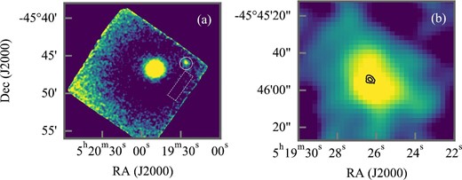
(a) FPMA exposure-corrected image smoothed by using a Gaussian with the standard deviation of |${4{^{\prime \prime}_{.}}8}$|. The circle and the rectangle indicate the source and the background regions, respectively. (b) Enlarged image around the western region overlaid with the contour of Chandra image. (Color online)
The brighter source at the center of the image is the Pictor A nucleus, the detailed spectral analysis of which was already reported in Kang, Wang, and Kang (2020). In addition to the nucleus, we see another X-ray source in the north-west. As shown in the enlarged image in panel (b) of figure 1, with overlaid contours of the Chandra image, we see that the hard X-ray source is well associated with the hotspot. The significance of this hard X-ray emission with NuSTAR was measured to be 30σ from the statistical error of the background.
To investigate the candidate hard X-ray emission of the hotspot, we evaluated the spatial properties quantitatively. We found that positions of the brightest pixels in FPMA and FPMB are |${2{^{\prime \prime}_{.}}5}$| and |${2{^{\prime \prime}_{.}}8}$| away from the position determined by Chandra, respectively. These are within the pointing uncertainty of NuSTAR of 8″ (Harrison et al. 2013).
The apparent size is measured on the un-smoothed image (i.e., the raw image of figure 1b) as 35″ in HPD, which is smaller than the NuSTAR PSF size of 58″ in HPD. Therefore, the major emission from the object is considered to be a point-like object for NuSTAR. Since the evaluated soft X-ray hotspot size is negligible compared to the PSF of NuSTAR, the obtained image size is consistent with the hotspot. In addition, there is no other bright X-ray source around the hotspot in the Chandra image as mentioned above. Therefore, we safely conclude that the observed source is a hard X-ray counterpart of the hotspot. This is the first time that a jet termination hotspot has been detected in the energy range above 10 keV.
3.2 Time variability analysis using Chandra data
Hardcastle et al. (2016) reported some interesting X-ray behavior—a month-scale flux decrease of the hotspot. They suggested that it could be caused by energy losses of the highest-energy electrons. However, the flux decrease is accompanied by a spectral hardening, which may imply a flux decrease in the low-energy band (see, Hardcastle et al. 2016; Thimmappa et al. 2020). Here, we carefully examined the unexpected increase of molecular contamination on the detector surface, which reduces the effective area below the 1 keV band. In fact, a position dependence of the contamination is reported, although the time variation at the typical aim point is calibrated and corrected with the CALDB file (Plucinsky et al. 2018).
We investigated the time variation of the count rate of the hotspot in low-energy (0.3–1.0 keV), which is sensitive to contamination, and high-energy (1.0–7.0 keV) bands for comparison separately. We divided the observation data into nine epochs, according to Hardcastle et al. (2016), to show the time history of count rates in figure 2. In the low-energy band, the count rates in epochs 4, 6, 8, and 9 are around |$20\%$| lower than those in the other epochs, while there is no significant fluctuation in the high-energy band.
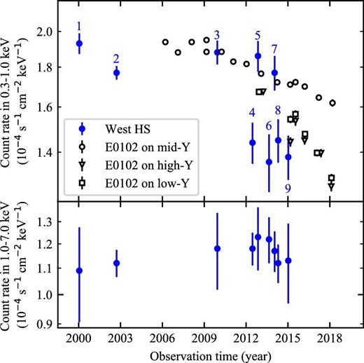
Count rates of the western hotspot and E0102. Upper panel: Low-energy band of 0.3–1.0 keV. Lower panel: High-energy band of 1.0–7.0 keV. The count rate of E0102 is scaled in comparison with the hotspot. The blue filled circle indicates the count rate of the hotspot and its number indicates a corresponding epoch. The open circle, open triangle, and open square indicate the E0102 at the mid-, high-, and low-Y positions, respectively. (Color online)
Figure 3 shows the source position on the detectors for each epoch. In epochs 4, 6, and 8, the hotspot is close to the chip gap or is observed by a different ACIS chip. In these cases, we cannot ignore the systematic uncertainties. To examine the apparent decrease in epoch 9, we also investigated the count-rate variation of a calibration source, the supernova remnant E0102, during this period. E0102 has been observed at three different locations on the detector, indicated as low-Y, mid-Y, and high-Y in figure 3. The obtained count rates are also shown in figure 2. We see the count rates on high- and low-Y positions have decreased since 2015. This trend implies that the contamination effect causes the apparent decrease of the count rates on low- and high-Y positions. The hotspot position in epoch 9 is near the high-Y location. Thus, we regard the apparent decrease in epoch 9 likely caused by artifacts (building-up contaminants). The hotspot’s location at epoch 8 is not exactly the same as that for E0102, but is located at the high-Y position where rapid increase of contaminants has been suggested. Therefore, the count-rate drop observed at epoch 8 would be caused not only by the effects of the chip gap but also by the possible contaminants. In this context, we argue that the flux decrease after epoch 8 might be affected by the detector response, particularly for the contaminants on the detector, although our argument does not completely exclude the flux variability reported in Hardcastle et al. (2016). It is important to evaluate the contamination build-up carefully, for more detailed investigations on the time variability. The results from the X-ray all-sky survey performed by eROSITA (Predehl et al. 2021) will provide us with an excellent opportunity for this purpose.
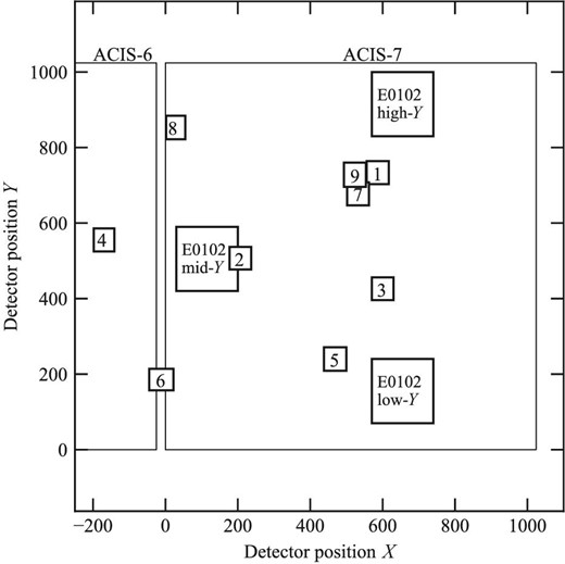
Detected positions of the hotspot and E0102 on the ACIS. The small square surrounding the number indicates the hotspot position in each epoch. The three middle squares indicate the E0102 positions of low-, mid-, and high-Y. The large squares drawn with a thin solid line indicate the ACIS chips 6 and 7.
3.3 Spectral analysis
3.3.1 XMM-Newton spectrum
We investigated the spectrum obtained from XMM-Newton’s second observation of Pictor A. The source spectrum was extracted from a circular region with a radius of 18″ centered at the brightness peak of the hotspot. The background spectrum was extracted from a nearby, source-free circular region with a radius of 36″, from which point sources detected by edetect_chain script are excluded. We adopted the same procedure of spectral extraction for MOS1 and PN. The source emission significantly exceeds the background one in the energy range of 0.2–10.0 keV in both MOS1 and PN. The spectral analysis hereafter were performed with XSPEC (Arnaud 1996) version 12.11.1 in HEAsoft package version 6.28.
We fitted the background-subtracted spectrum with an absorbed power-law model, described as tbabs*pegpwrlw in XSPEC, using χ2 statistics. In the fitting, we fixed the hydrogen column density to the Galactic value of NH = 3.6 × 10²⁰ atoms cm−2 obtained from HI4PI (HI4PI Collaboration 2016).1 The solar abundance table we used in XSPEC was obtained from Anders and Grevesse (1989). Figure 4 shows the spectra and the best-fitting models, and the best-fitting parameters and fitting range are summarized in table 2. The models reproduce the spectra well, with χ2/d.o.f. = 97/90 and 197/181 for spectra obtained by MOS1 and PN, respectively.
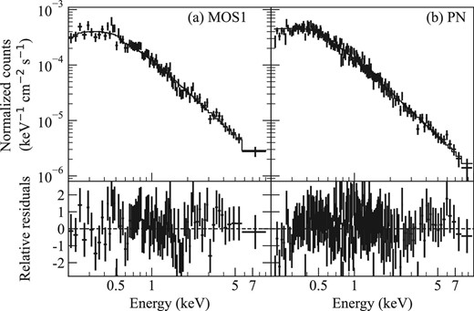
Background-subtracted spectra of the XMM-Newton detectors (cross) and best-fitting models (solid line). (a) MOS1. (b) PN.
Best-fitting parameters and |$90\%$| confidence error of each detector spectrum.
| Instruments | Fitting range* | Total flux† | Common flux‡ | Γ§ | NH|| | χ2/d.o.f. |
|---|---|---|---|---|---|---|
| XMM-Newton | 0.2–10 keV | |||||
| MOS1 | 0.86 ± 0.03 | 0.18 ± 0.01 | 2.02 ± 0.05 | 3.6 (fixed) | 97/90 | |
| PN | 0.89 ± 0.02 | 0.181 ± 0.009 | 2.05 ± 0.03 | 3.6 (fixed) | 197/181 | |
| MOS1+PN | 0.88 ± 0.02 | 0.181 ± 0.007 | 2.04 ± 0.03 | 3.6 (fixed) | 290/268 | |
| Chandra | 1.5–7.0 keV | |||||
| ACIS | 0.347 ± 0.007 | 0.185 ± 0.006 | 2.09 ± 0.04 | 3.6 (fixed) | 226/235 | |
| NuSTAR | 3–20 keV | |||||
| FPMA | 0.46 ± 0.05 | 0.20 ± 0.03 | 2.0 ± 0.3 | 3.6 (fixed) | 15.0/21 | |
| FPMB | 0.45 ± 0.06 | 0.16 ± 0.03 | 1.6 ± 0.4 | 3.6 (fixed) | 23.5/23 | |
| FPMA+B | 0.45 ± 0.04 | 0.18 ± 0.02 | 1.8 ± 0.2 | 3.6 (fixed) | 42.3/44 | |
| All | 0.2–20 keV | 1.05 ± 0.01 | 0.189 ± 0.004 | 2.02 ± 0.02 | 3.6 (fixed) | 577/551 |
| 0.2–20 keV | 1.07 ± 0.02 | 0.185 ± 0.004 | 2.07 ± 0.03 | 4.6|$^{+0.5}_{-0.5}$| | 563/550 |
The energy range used for the fitting.
Unabsorbed flux within fitting range in units of 10−12 erg s−1 cm−2.
Unabsorbed flux within 3–7 keV in units of 10−12 erg s−1 cm−2.
Photon Index of power-law model.
Hydrogen column density in unit of 1020 atoms cm−2.
We compared the confidence contours, to check the consistency between the MOS1 and PN spectra. As shown in figure 5, the contours are consistent with each other at a 68% confidence level. Then, we fitted the MOS1 and PN spectra simultaneously. The best-fitting parameters and the confidence contours are shown in figure 5 and table 2, respectively. There is no significant difference between the joint and individual fittings.
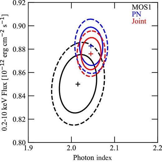
Confidence contours for the 0.5–7 keV flux and photon index of the MOS1 (black), PN (blue), and MOS1 and PN jointed (red) spectrum fitting. The solid and dashed lines indicate |$68\%$| and |$90\%$| confidence levels, respectively. The crosses indicate best-fitting parameters. (Color online)
3.3.2 Chandra spectrum
To improve the photon statistic, we utilized the Chandra spectra. We adopted the circular region with a radius of 8″ and the annulus region with the inner and outer radii of 12″ and 20″ for the source and background regions, respectively. We used the spectrum above 1.5 keV, to avoid the possible contamination effect. For a simplification, we combined the spectra in epochs 1–9 using the addascaspec command. We fitted the combined spectrum with the absorbed power-law model the same as for the XMM-Newton spectrum. The model reproduced the spectrum well, with the best-fitting chi-square statistics of χ2/d.o.f. = 226/235. The best-fitting parameters are summarized in table 2. The derived parameters are consistent with the analysis of early Chandra data in Wilson, Young, and Shopbell (2001).
3.3.3 NuSTAR spectrum
To investigate the hard X-ray property of the western hotspot, we analyzed the NuSTAR spectrum. As shown in figure 1, we employed a circular region with a radius of 50″ centered at the centroid of the hard X-ray brightness distribution of the western hotspot and a rectangular area in the same detector chip for the source and background, respectively. We extracted the source and background spectra via the nuproducts script, which also generates the response matrix functions and the auxiliary response files. Figure 6 shows the source and background spectra of the FPMA and FPMB. We see significant emissions from the hotspot in the energy range of 3–20 keV, in both detectors.
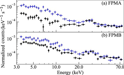
Normalized counts. Source (crosses) and background spectra (filled squares) of FPMA and FPMB. (Color online)
We fitted the background-subtracted spectra with the absorbed power-law model the same as for XMM-Newton and Chandra spectra. Figure 7 shows the background-subtracted spectra and the best-fitting models. The best-fitting parameters are summarized in table 2. The models reproduce the spectra well, with χ2/d.o.f. = 15.3/21 and 23.5/23 for FPMA and FPMB, respectively, although the FPMA spectrum prefers a slightly softer photon index of Γ = 2.0 ± 0.3 to that of FPMB, Γ = 1.6 ± 0.4. To investigate the spectral difference, we calculated the confidence contours between the flux and photon index, as shown in figure 8. The parameters are consistent with each other to within a |$68\%$| confidence level. Then, we performed a joint fitting. The best-fitting parameters and confidence contours are shown in table 2 and figure 8, respectively. We confirmed that the joint fitting reproduces the FPMA and FPMB spectrum well, with χ2/d.o.f. = 42.3/44, and the best-fitting parameters are consistent with those derived from individual fittings.
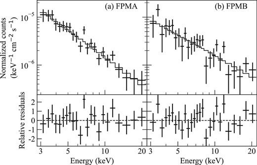
Background-subtracted spectrum (crosses) and best-fitting model (solid line) of FPMA and FPMB.
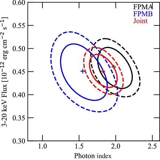
Confidence contours for the 3–20 keV flux and photon index of the FPMA (black), FPMB (blue), and FPMA and FPMB joint (red) spectrum fitting. The solid and dashed lines indicate |$68\%$| and |$90\%$| confidence levels, respectively. The crosses indicate best-fitting parameters. (Color online)
3.3.4 Wide-band X-ray spectra
Figure 9 shows the hotspot spectra obtained by NuSTAR, XMM-Newton, and Chandra. The spectra are connected smoothly, as expected from table 2 showing that the best-fitting parameters are almost consistent among different satellites within the calibration uncertainties (Madsen et al. 2017). Therefore, we performed a simultaneous fit using all the data. The data cover a broader energy range (0.2–20 keV) and have higher photon statistics than ever for this object. We simultaneously fitted the spectra by the absorbed power-law model with the fixed column density. The best-fitting model reproduced the spectrum well, with χ2/d.o.f. =577/551, as shown in figure 9. The derived best-fitting parameters, summarized in table 2, are consistent with the parameters derived from the individual spectrum.
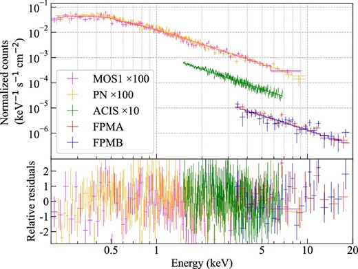
Spectra, best-fittng absorbed power-law models and relative residuals of FPMA (red), FPMB (blue), ACIS (green), MOS1 (magenta), and PN (orange). For better visibility, the counts of MOS1 and PN are scaled up 100 times and counts of ACIS are scaled up 10 times. (Color online)
In order to improve the fit, we fitted the data with the same model by allowing the hydrogen column density to vary. The best-fitting model eliminated slight residuals in 0.2–0.3 keV. The derived parameters are shown in table 2. This model gives χ2/d.o.f. = 563/550, indicating a statistically significant improvement with a null hypothesis probability of 2 × 10⁻⁴ calculated by the F-test. The derived column density of NH = (4.6 ± 0.5) × 1020 atoms cm−2 is slightly higher than the Galactic value from HI4PI Collaboration (2016). In contrast, the others are statistically consistent with the case of the fixed column density. We see no spectral break in the wide-band spectra from which we excluded the Chandra spectrum below 1.5 keV.
As an advanced investigation, we searched for a spectral curvature. If the X-ray spectrum originates from an electron synchrotron emission, a high-energy exponential cut-off is naturally expected to correspond to the maximum energy of electrons. We examined the spectrum with a simple cut-off power-law model of tbabs*cutoffpl, and obtained the cut-off energy at >54 keV in the statistical significance level of |$5\%$| with χ2/d.o.f. = 608/552. As the energy of 54 keV is above the energy coverage of our data (0.2–20 keV), hereafter we adopt 20 keV as our conservative lower limit of the cut-off energy.
It is interesting to note the analogy with studies of supernova remnants (SNRs). Although X-ray synchrotron spectra in SNRs look similar to that observed in the Pictor A’s western hotspot, they are interpreted differently—the X-rays of SNRs are generally believed to be tails of power-law emission with an exponential cut-off below ∼1 keV (see reviews in Helder et al. 2012; Vink 2012, and references therein). For a recent example, in Kepler’s SNR, Nagayoshi et al. (2021) revealed a power-law spectrum up to 30 keV, similar to the hotspot, and showed that it is reproduced by a power law with an exponential cutoff at ∼0.5 keV. Therefore, one may think that the same interpretation could be applicable to the hotspot. However, the X-ray spectrum cannot be represented by the model of tbabs*srcut, which is the simple cut-off power-law model often used for SNRs if we assume cut-off energy below 20 keV. Hence, the cut-off energy would be higher than 20 keV for this model, too.
4 Discussion
4.1 Origin of the X-ray emission
The X-ray emission mechanism of the Pictor A western hotspot has been discussed since the first clear detection by Chandra in Wilson, Young, and Shopbell (2001). The X-ray spectrum is brighter and harder than the extrapolation of the radio to optical synchrotron spectrum. It is known to be challenging to explain the X-ray via the SSC process because the X-ray and synchrotron radio emissions have different spectral indices and emission regions (Wilson et al. 2001; Thimmappa et al. 2020). It is considered plausible that the X-ray originates from a synchrotron emission of the electrons that is different from that corresponding to the radio to optical emission (see, e.g., Wilson et al. 2001; Hardcastle et al. 2004, 2016; Thimmappa et al. 2020).
Tingay et al. (2008) proposed that X-rays originate from the fine structures around the radio brightness peak, and Hardcastle et al. (2016) supported the scenario based on the time scale of the flux decrease. However, according to Hardcastle et al. (2016) and Thimmappa et al. (2020), a major part of the X-ray emission locates away from the radio fine structure. In addition, as has been checked in subsection 3.2, an instrumental effect (i.e., contamination) may contribute the observed flux drop, especially on the soft energy band, and thus the intrinsic variability may be reduced. Therefore, as pointed out by Thimmappa et al. (2020), it seems to be more reasonable that most of the X-rays are emitted from the thin shock front region.
4.2 Accelerated electron energy distribution
Hotspots are believed to be sites of particle acceleration via the relativistic shock and a possible ultra-high-energy cosmic-ray accelerator (Hillas 1984; Kotera & Olinto 2011). Therefore the observational electron spectrum of the hotspot potentially provides us with essential information for the relativistic shock study.
The X-ray observations in a wide energy range with high statistics revealed the featureless power-law spectrum in 0.2–20 keV. The spectrum indicates that the X-ray emitting electrons are not responsible for the higher end of energy distribution (see section 3). Therefore we estimated the X-ray emitting electron’s energy index (p), which is the important information on the acceleration process, from the X-ray photon index (Γ = 2.07 ± 0.03) to be p = 2Γ − 1 = 3.14 ± 0.06.
Several authors (e.g., Wilson et al. 2001; Aharonian 2002) have already pointed out the same electron energy index of the hotspot. However, the low statistics due to the only observation being that by Chandra allowed various X-ray spectral shapes. Our study tightly determines the X-ray spectral shape and excludes the cut-off or cooling break feature in the X-ray band.
We compared the maximum electron energy to blazars, which have spectral and environmental similarities with hotspots. Some observational and analytical studies estimated the maximum electron energy to be up to only a few TeV even in the TeV gamma-ray emitting blazars, which are believed to have the highest value among some types of blazar (see, e.g., Inoue & Takahara 1996; Kataoka et al. 1999; Kino et al. 2002; MAGIC Collaboration 2020). Therefore the synchrotron X-ray in the hotspots may reflect the highest energy electron in the AGN jet system.
For further investigations, we need to detect a higher energy spectrum and or other hotspots than in this study. Due to both lower X-ray flux and smaller angular offset from the nucleus in most hotspots than in the Pictor A western hotspot, it may be difficult for NuSTAR to detect other hotspots. We anticipate that future hard X-ray missions, which have better angular resolution and sensitivity than those of NuSTAR, for example, FORCE (Nakazawa et al. 2018), will vigorously promote this kind of study.
Acknowledgements
We thank Mr. Yuki Imai for help in the NuSTAR data analysis and Dr. Naoki Isobe for valuable comments. We deeply appreciate Observational Astrophysics Institute at Saitama University for supporting the research fund.
Footnotes
The NH value is obtained at the website 〈https://heasarc.gsfc.nasa.gov/cgi-bin/Tools/w3nh/w3nh.pl〉.
