


Abstract
Alkali metal lines are one of the most important key opacity sources for understanding exoplanetary atmospheres because the Na i resonance doublets are thought to be the cause of low albedo, as the alkali metal’s wide line wings absorb almost all of the incoming stellar irradiation. High-resolution transmission spectroscopy of Na absorption lines can be used to investigate the temperature of the thermosphere of hot Jupiters, which is increased by stellar X-ray and extreme-ultraviolet irradiation. We applied high-resolution transmission spectroscopy to the ultra-hot Jupiter WASP-76 b with the High Dispersion Spectrograph (HDS) on the Subaru 8.2 m telescope. We report the detection of strong Na D excess absorption with line contrasts of |$0.42 \pm 0.03\%$| (D1 at 5895.92 Å) and |$0.38\pm 0.04\%$| (D2 at 5889.95 Å), full width at half maximum values of 1.63 ± 0.13 Å (D1) and 1.87 ± 0.22 Å (D2), and equivalent widths of (7.29 ± 1.43) × 10−3 Å (D1) and (7.56 ± 2.38) × 10−3 Å (D2). These results show that the Na D absorption lines are shallower and broader than those in previous work, whereas the absorption signals over the same passband are consistent with those in previous work. We derive the best-fitting isothermal temperature of 3700 K (without rotation) and 4200 K (with rotation). These results suggest the possibility of the existence of a thermosphere because the derived atmospheric temperature is higher than the equilibrium temperature (∼2160 K).
1 Introduction
Previous observations have found a number of hot Jupiters, which are gaseous planets that orbit close to a star, unlike our solar system. Although hot Jupiters can be relatively easily detected and investigated because of their large signal, their formation and evolution are not fully understood. It is thus important to obtain detailed information about their atmospheric composition and temperature structure.
In the last two decades, our understanding of exoplanetary atmospheres has advanced considerably through spectroscopic observations during planetary transit events. Such observations are referred to as transmission spectroscopy. Alkali metal lines are one of the most important key opacity sources because the Na i resonance doublets are thought to be the cause of generally low albedos, as the alkali metal’s wide line wings absorb almost all of the incoming stellar irradiation (Seager & Sasselov 2000; Brown 2001; Barman et al. 2001; Hubbard et al. 2001).
High-resolution transmission spectroscopy can be used to investigate the upper atmosphere based on the centers of absorption lines. In particular, Na absorption in the line core makes it possible to investigate a thermosphere where the temperature is increased by stellar X-ray and extreme-ultraviolet (EUV) irradiation and there is atmospheric escape (Lammer et al. 2003; Yelle 2004; Vidal-Madjar et al. 2011; Koskinen et al. 2013). Na absorption has been detected with high-resolution spectroscopy for 10 hot Jupiters and one hot Neptune (e.g., Wyttenbach et al. 2015, 2017; Wood & Maxted 2011; Burton et al. 2015; Casasayas-Barris et al. 2017, 2018; Hoeijmakers et al. 2019, 2020; Seidel et al. 2019; Chen et al. 2020; Seidel et al. 2020a); however, there are some differences in these results that are not fully understood because the parameters vary between planets. To understand the atmospheric structures of hot Jupiters better and explain these differences, it is necessary to apply high-resolution spectroscopy to observe the Na absorption lines for a greater number of hot Jupiters.
There is a classification system that roughly divides hot Jupiters into two types based on the incident flux (equilibrium temperature of a planet) (Fortney et al. 2008). For an “ultra-hot Jupiter” with an equilibrium temperature of over 2000 K, it is predicted that TiO/VO absorption is governed by the optical wavelength and that Na absorption lines cannot be detected (Fortney et al. 2010). However, recent observations using transit photometry and low/high resolution spectroscopy detected many alkali lines and/or the Balmer series of H and/or TiO/VO in some ultra-hot Jupiters, revealing differences in their atmospheres (e.g., Sing et al. 2013; Burton et al. 2015; Evans et al. 2016; Sedaghati et al. 2017; Jensen et al. 2018; Casasayas-Barris et al. 2018; Wyttenbach et al. 2020; Hoeijmakers et al. 2020). To investigate these differences, observations of the atmosphere in more ultra-hot Jupiters are needed.
WASP-76 b, which is around an F-type star, was confirmed by West et al. (2016). This planet is an inflated ultra-hot Jupiter with a radius of 1.854 RJ, a mass of 0.894 MJ, an equilibrium temperature of 2228 K, and an orbital period of ∼1.8 d. The parameters of the WASP-76 system are listed in table 1. Because the WASP-76 b system has a bright host star and a large scale height, its atmosphere can be investigated.
Parameters of the WASP-76 system.
| Parameter | Value |
|---|---|
| Star | WASP-76 |
| V mag | 9.5 |
| Spectral type | F7* |
| Rs (Rsun) | 1.756 ± 0.071† |
| Teff (K) | 6329 ± 65† |
| Transit | |
| T0 (UTC) | 2456107.85507 ± 0.00034* (HJD) |
| P (d) | 1.809886 ± 0.000001* |
| Duration (hr) | 3.694 ± 0.019* |
| Impact parameter: b | 0.14|$^{+0.11}_{-0.09}$|* |
| Semimajor axis: a (au) | 0.0330 ± 0.0005* |
| Planet | WASP-76 b |
| Mp (MJ) | 0.894|$^{+0.014}_{-0.013}$|† |
| Rp (RJ) | 1.854|$^{+0.077}_{-0.076}$|† |
| Tp, A = 0 (K) | 2228 ± 122† |
| g = G|$M_{\rm p}/R_{\rm p}^2$| (cm |$\rm {s^{-2}}$|) | ∼ 645 |
| H† (km) | ∼ 1249 |
In 2019, two studies reported the detection of Na absorption lines in the atmosphere of WASP-76 b with high-resolution spectroscopy (Seidel et al. 2019; Žák et al. 2019). These studies used the same data (observed with HARPS in three nights) but different analysis methods. Both detected Na absorption, but the depth and full width at half maximum (FWHM) values were different. Furthermore, Ehrenreich et al. (2020) confirmed the existence of iron, which condenses at the nightside, from the asymmetry of the absorption signal of atomic iron obtained with the Echelle Spectrograph for Rocky Exoplanets and Stable Spectroscopic Observations (ESPRESSO) at the European Southern Observatory’s Very Large Telescope (VLT). In space, the low-resolution spectra (transmission and emission spectra) of WASP-76 b were observed several times with STIS, Wide Field Camera 3 (WFC3) of the Hubble Space Telescope (HST), and Spitzer. The results were used to calculate a temperature–pressure (T-P) profile at the terminator and dayside, and the existence of TiO and H2O was detected in the transmission spectra, a strong CO emission feature was found in the secondary eclipse spectra, and sodium was found at 2.9σ significance (Edwards et al. 2020; Fu et al. 2021; Lothringer et al. 2020; von Essen et al. 2020). In addition, it is found that WASP-76 has a companion star whose temperature is 4824 K and which is separated by about |${0^{\prime \prime }.436}$| (Bohn et al. 2020; Southworth et al. 2020). Because this companion cannot separate from the host star in photometry, it affects HST data. Most recently, the transmission spectra of two primary transits were observed with ESPRESSO; the atomic absorption lines of Li i, Na i, Mg i, Ca ii, Mn i, K i, and Fe i were detected (Tabernero et al. 2021).
Thanks to the previous studies, many atoms and molecules are detected in the atmosphere of WASP-76 b. The existence of the temperature inversion is estimated from the detection of atoms and molecules such as TiO/VO, but it is not confirmed in the retrieval fitting with transmission spectra of HST. In high resolution, Seidel et al. (2019) tried to fit their data with the theoretical transmission spectrum, but they could not adjust the line profile.
In the present study, we show the high-resolution transmission spectra of WASP-76 b observed with the Subaru 8.2 m telescope and High Dispersion Spectrograph (HDS; Noguchi et al. 2002) and fit them with our theoretical transmission spectra considering equilibrium chemistry, namely thermal ionization of sodium. The rest of this paper is organized as follows. In sections 2 and 3, we describe our observations and the procedure used for data reduction, respectively. In section 4, we show the results of the transmission spectrum and atmospheric absorption. In section 5, we discuss the effect of instrumental variation and conduct a comparison with model spectra. In section 6, we summarize this work.
2 Observations
On 2018 September 10 UT, we observed the F-type star WASP-76 during the transit of its hot Jupiter WASP-76 b with Subaru/HDS. The wavelength range was set to cover 5430–8100 Å, which is a non-standard setup for HDS, using a red cross-disperser grating with a central wavelength of 6700 Å to observe the Na (D1 = 5895.92 Å; D2 = 5889.95 Å) and K absorption lines simultaneously. The slit width was set to |${0.4^{\prime \prime }}$|, corresponding to a spectral resolution of ∼90000.
Because the transit duration of the planet is about 3.7 hr from 10 : 41 UT to 14 : 23 UT, observation started at 8 : 22 UT and finished at 15 : 41 UT. We obtained a total of 35 out-of-transit spectra and 35 in-transit spectra of WASP-76 b with an exposure time of 300 s. The signal-to-noise ratio (SNR) of the extracted spectra was about 86 pixel−1 on average and about 23 pixel−1 for the line core of the Na D lines at each frame.
To obtain the telluric spectra, we observed the rapid rotator HR 8634 (B8V, vsin i = 185 km s−1; Glebocki et al. 2000) from 5 : 19 UT to 8 : 11 UT. We obtained 180 exposures of 5 s each for the star. The SNR of the extracted spectra was about 158 pixel−1 on average at each frame.
The Earth’s atmospheric conditions during the observation of WASP-76 and HR 8634 are shown in figure 1. The precipitable water vapor (PWV), which refers to the depth of water vapor in a column of the atmosphere, was measured by the Caltech Submillimetre Observatory radiometer at 225 GHz from the linear relation between the measurable PWV in millimeters and the opacity at 225 GHz (Dempsey et al. 2013). The average PWV was about 1.32 mm, which means that the atmosphere is dry. This value was relatively stable during the observations. Table 2 summarizes the observation log.
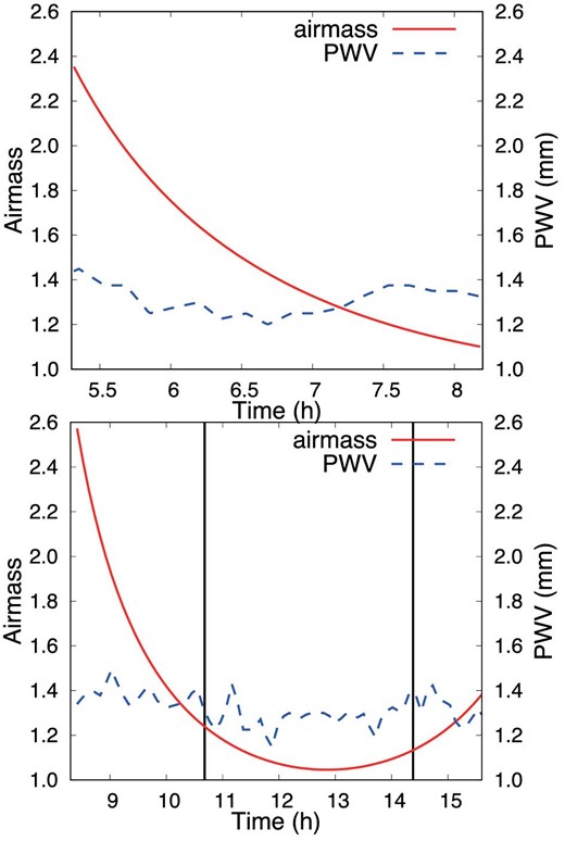
Earth’s atmospheric condition during the observation of HR 8634 (top) and WASP-76 (bottom) on 2018 September 10 UT. The vertical lines represent the start (left) and end (right) of transit. The variations in the airmass and PWV are represented by the red and blue lines, respectively. (Color online)
Observation log.
| Object | Date | Obtained spectra | Exp. time | Airmass | PWV |
|---|---|---|---|---|---|
| (UT) | In-transit + out-of-transit | (s) | (mm) | ||
| WASP-76 | 2018/09/10 | 35 + 35 | 300 | 1.05–2.57 | 1.32 ± 0.07 |
| Object | Date | Obtained spectra | Exp. time | Airmass | PWV |
|---|---|---|---|---|---|
| (UT) | In-transit + out-of-transit | (s) | (mm) | ||
| WASP-76 | 2018/09/10 | 35 + 35 | 300 | 1.05–2.57 | 1.32 ± 0.07 |
3 Data reduction
To extract the transmission spectra, the one-dimensional spectral flux as a function of wavelength was extracted from the two-dimensional images recorded on a CCD detector and the telluric spectrum, stellar spectrum, and instrumental variation were removed. The first data reduction was performed using the Image Reduction and Analysis Facility (IRAF).1 Other procedures are described below.
3.1 Telluric correction
Telluric absorption lines were superposed on to the stellar spectrum observed from the ground. Many telluric water vapor absorption lines appear around Na D lines. There are three main methods for removing these telluric absorption lines. One uses the spectra of a rapidly rotating star (a rapid rotator) (e.g., Winn et al. 2004; Kawauchi et al. 2018), one uses the telluric lines in out-of-transit spectra (e.g., Astudillo-Defru & Rojo 2013; Wyttenbach et al. 2015), and one uses the “molecfit” program (Smette et al. 2015; Kausch et al. 2015) which combines model spectra of Earth’s atmosphere with the local weather profile (e.g., Hoeijmakers et al. 2020; Seidel et al. 2020a).
However, because the rapid rotator has a broad absorption feature, the continuum feature is not the same as those for neighboring orders. Therefore, we could not use the correction method used for the stellar spectra. To create normalized spectra, we divided the spectra every 40 pixels (5 × FWHM), selected the ninth largest value (|$80\%$| from the bottom) as the value of the central wavelength, and fitted these values using cubic spline (figure 2). The divided pixel and the used value are decided by changing at each FWHM (∼0.15 Å) and at each |$10\%$|. Based on these normalized spectra, we measured the optical depth around Na absorption lines. Using this optical depth, we corrected the telluric spectra in WASP-76 b spectra to the noise level (figure 3).
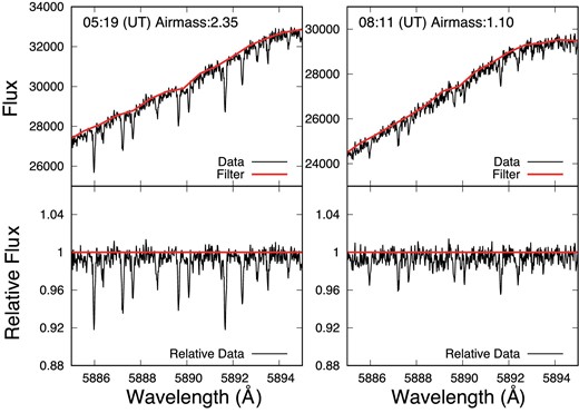
Top: Spectra of the reference star HR8634 (black) and the calculated filter to remove the continuum (red) at two different times. Bottom: Relative spectra (black) and the horizontal line of 1. (Color online)
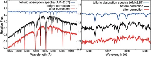
One of the HDS spectra of WASP-76 b before (black) and after (red) telluric correction. The blue lines show the telluric absorption spectra. The right-hand panel is a zoom-in of the left-hand panel. (Color online)
3.2 Correction for instrumental variation
The stellar spectrum observed with an echelle spectrograph such as Subaru/HDS has a blaze function for each observed order. However, in reality, this blaze function also has a time variation. This time variation can reduce the accuracy of flux correction using a standard star. It is considered that this time variation is caused by the changes in the optical path of the telescope and is related to the telescope position during observation and/or its focal length. However, because this time variation is not fully understood, it cannot be corrected for systematically.
The target spectrum can be fitted using the continuum region to remove the effects of the blaze function. However, the blaze function cannot be fitted with high accuracy around broad and deep absorption lines such as Na D lines. For our observations, high-accuracy flux correction is necessary because the absorption lines of the exoplanet atmosphere are quite sensitive to differences in the continuum level. Therefore, we used the correction method adopted by Winn et al. (2004) and Narita et al. (2005) because it has a relatively high accuracy [the remaining instrumental effect is |$\sim\! 0.1\%$| with 2 Å passband reported by Narita et al. (2005)].
In their analysis, Winn et al. (2004) used all 4100 pixels in the order while Narita et al. (2005) only used only about 1000 pixels around the Na D absorption lines to prevent the dilution of real signals. In our analysis, we used about 2300 pixels to cover the region of the reference band (5874.89–5886.89 Å and 5898.89–5910.89 Å).
We estimated the temporal variation by interpolating those obtained for neighboring orders based on the ratio between the spectrum that combines all spectra and the spectra at a given time. To estimate the temporal variation with more accuracy than that in previous studies, we removed outliers from neighboring orders and smoothed these orders by an average of 40 pixels. We used orders 99 and 103 to correct for the time variation of order 101, which has Na D absorption lines, because order 100 contains different time variations compared to the other orders (figure 4).
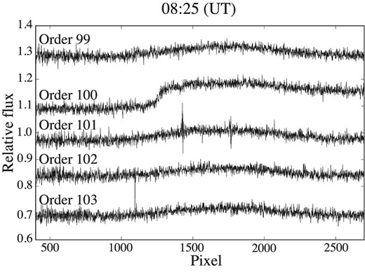
Ratio between the template spectrum and the spectra for orders 99, 100, 101, 102, and 103. The variation of order 100 is different from those of the other orders.
Figure 5 shows the original and corrected spectra and the ratio between the template spectrum and the spectrum at a given time. These results show that all spectra are well corrected (the residual was around zero for all wavelengths).
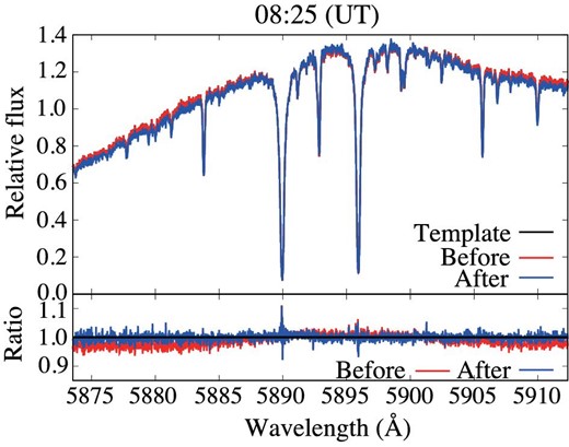
Blaze correction at certain time points. The upper panel shows the template spectrum (black) and the spectra before (red) and after (blue) the blaze function correction. The bottom panel shows the ratio of the template spectrum to the spectra before (red) and after (blue) the blaze function correction. The black line in the bottom panel indicates a ratio of one. (Color online)
3.3 Removal of stellar spectrum
4 Results
4.1 Transmission spectrum
The transmission signal was too faint to detect absorption lines. We thus combined the in-transit spectra to obtain the transmission spectrum. However, the absorption lines of the planet’s atmosphere are shifted during transit because the planet orbits around its star.
This allowed us to identify the Na D lines visually (figure 6). We estimated the transmission spectrum with a Gaussian fitting of each Na D line using Markov chain Monte Carlo (MCMC) analysis using the ensemble sampler “emcee” (Foreman-Mackey et al. 2013). We fitted the observed spectrum with a flat line and two Gaussians between 5885 and 5900 Å and measured line contrasts of |$0.40 \pm 0.03\%$| (D1) and |$0.38 \pm 0.05\%$| (D2) and FWHM values of 1.52 ± 0.13 Å (D1) and 1.65 ± 0.29 Å (D2). We also calculated equivalent widths (EWs) of (6.47 ± 1.42) × 10−3 Å (D1) and (6.66 ± 3.13) × 10−3 Å (D2).
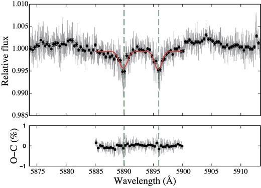
Transmission spectrum corrected by planet radial velocity before correction of a wide trend. The red line indicates the fitting result obtained with a flat line and two Gaussians between 5885 and 5900 Å (we could not fit between 5873.7 and 5913.4 Å). The bottom panel shows the residuals of fitting. (Color online)
We found a wide trend around the Na absorption lines. To investigate the cause of this feature, we separated the template stellar spectrum into two types, namely spectra summed before and after transit, respectively. The left-hand side of figure 7 shows the transmission spectrum [Tin/before(λ)] based on the template stellar spectrum summed before transit, and the right-hand side of figure 7 shows the transmission spectrum [Tin/after(λ)] based on the template stellar spectrum summed after transit. The wide trend appears for only Tin/after(λ). Therefore, this trend results from the data after transit.
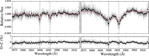
Top panels show the spectrum during transit divided by that before transit (left) and the spectrum during transit divided by that after transit (right). The red line indicates the fitting result obtained with a flat line and two Gaussians between 5873.7 and 5913.4 Å. The bottom panels show the residuals of fitting. (Color online)
WASP-76 has a binary with a separation of |${0^{\prime \prime }.436}\pm {0^{\prime \prime }.003}$| and position angle is |${215.9D} \pm {0.4D}$| (Bohn et al. 2020). From the image viewer at each observation time, it was found that part of the data during transit included this binary star. However, this did not cause the wide trend around the Na absorption lines because the time variation of this trend is different from the period when the binary was in the slit.
Because this trend is not the atmospheric signal, we corrected the variation with linear interpolation in each frame except around Na absorption lines (5887.22–5897.98 Å) to preserve the atmosphere’s feature, and combined the transmission spectrum frames to create the transmission spectrum (figure 8). Line contrasts of |$0.42 \pm 0.03\%$| (D1) and |$0.38 \pm 0.04\%$| (D2), FWHM values of 1.63 ± 0.13 Å (D1) and 1.87 ± 0.22 Å (D2), and EWs of (7.29 ± 1.43) × 10−3 Å (D1) and (7.56 ± 2.38) × 10−3 Å (D2) were obtained for this transmission spectrum. Our absorption lines are wider than those reported in previous studies (table 3).
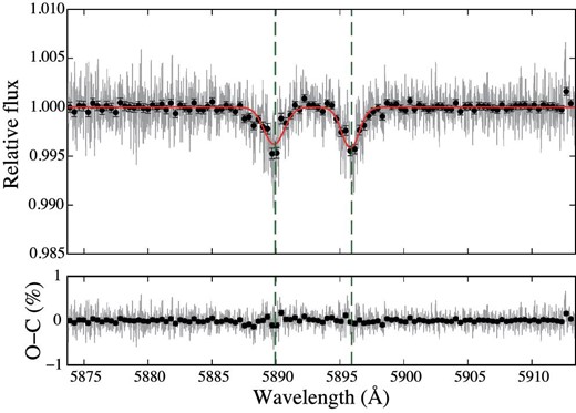
Transmission spectrum after correction of a wide trend. The red line indicates the fitting result obtained with a flat line and two Gaussians between 5873.7 and 5913.4 Å. The bottom panel shows the residuals of fitting. (Color online)
Results.
| Our results | Seidel et al. (2019) | |||
| D1 | D2 | D1 | D2 | |
| Line contrast (%) | 0.42 ± 0.03 | 0.38 ± 0.04 | 0.508 ± 0.053 | 0.373 ± 0.091 |
| FWHM (Å) | 1.63 ± 0.13 | 1.87 ± 0.22 | 0.680 ± 0.128 | 0.619 ± 0.174 |
| Tabernero et al. (2021) | ||||
| D1 (T1) | D2 (T1) | D1 (T2) | D2 (T2) | |
| Line contrast (%) | 0.385 ± 0.051 | 0.449 ± 0.049 | 0.294 ± 0.042 | 0.246 ± 0.037 |
| FWHM (Å) | 0.417 ± 0.065 | 0.483 ± 0.061 | 0.464 ± 0.081 | 0.623 ± 0.112 |
Recently, it was reported that the Rossiter–McLaughlin (RM) effect and center-to-limb variation (CLV) affect the Na absorption estimated from high-resolution spectra (Czesla et al. 2015; Yan et al. 2017; Borsa & Zannoni 2018).
The RM effect depends on the rotation velocity of the star and where the planet transits on the surface of the star. As WASP-76 b is in polar orbit (Brown et al. 2017) and WASP-76 is a slow rotator, the RM effect is small. The feature of the RM effect was not detected at the noise level of |$0.01\%$| (Seidel et al. 2019). This means that the RM effect in the WASP-76 system is under the photon noise level in our results (continuum: |$\sim\! 0.01\%$|, line core: |$\sim\! 0.04\%$| per pixel) and can thus be ignored.
The CLV effect depends on the stellar temperature and the impact parameter of the planet. As WASP-76 is an F-type star (Teff = 6250 K), its CLV effect is less than that for earlier-type stars. According to Yan et al. (2017), the CLV effect is about |$0.25\%$| for an integral passband of 0.75 Å because the impact parameter of WASP-76 b is 0.14. This value is below the photon noise level in our results (∼0.038) and thus the CLV effect can be ignored.
4.2 Calculation of atmospheric absorption
We detected the Na absorption lines of the planet atmosphere from the transmission spectrum of WASP-76 b.
By comparing the average of the integrated value in the left-hand continuum region, which ranges from 5874.89 to 5886.89 Å, and that in the right-hand continuum region, which ranges from 5898.89 to 5910.89 Å, we estimated the planetary absorption around the Na D lines for each passband (0.2–10 Å in 0.1 Å steps) for the original and corrected spectra and compared the results with those in a previous work (Seidel et al. 2019) (figure 9). No differences were found between the Na D1 and NaD2 lines and the absorption signal for the corrected spectra is mostly consistent with that in the previous work.
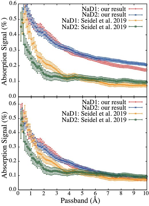
Absorption of Na D1 (red) and Na D2 (blue) for each integral passband for our results before (top) and after (bottom) correction and for the results of Seidel et al. 2019 (Na D1: orange, Na D2: green). (Color online)
We also created transmission light curves integrated over the passbands of 0.75, 1.5, and 3.0 Å (figure 10) using the same continuum region. The results show a significant reduction during transit for all passbands.
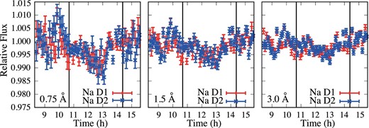
Transmission light curves before correction integrated over passbands of 0.75 (left), 1.5 (center), and 3.0 (right) Å around Na D1 (red) and Na D2 (blue) lines. The vertical lines represent the start (left) and end (right) of transit. (Color online)
5 Discussion
5.1 Effect of instrumental variation after correction
Our results include instrumental variation and have a wide trend. To confirm our correction of these variations, we used the empirical Monte Carlo (EMC) method as done by Redfield et al. (2008).
We created a template stellar spectrum (Fstar) and a master in-transit spectrum (that is, a normalized spectrum that combines all spectra during transit, Fmaster-in) with randomly extracted frames from the frames of out-of-transit data only (|$T_{\rm out{-}out}$|) and the frames of in-transit data only (|$T_{\rm in{-}in}$|). We also created Fstar with randomly extracted frames from the frames of out-of-transit data only and |$F_{\rm master{-}in}$| with randomly extracted frames from the frames of in-transit data only (|$T_{\rm in{-}out}$|). Note that the number of extracted frames is the same as that when we created the original spectra (Fstar: 35 frames, |$F_{\rm master{-}in}$|: 35 frames). We iterated the above process 20000 times and examined the distribution of the absorption signal at each integral width (3 and 6 Å).
The absorption signals of |$T_{\rm in{-}in}$|, |$T_{\rm out{-}out}$|, and |$T_{\rm in{-}out}$| are |$-0.000 \pm 0.052\%$|, |$-0.001 \pm 0.060\%$|, and |$0.238 \pm 0.057\%$| for 3 Å, and |$0.000 \pm 0.040\%$|, |$- 0.001 \pm 0.050\%$|, and |$0.129 \pm 0.044\%$| for 6 Å (figure 11). As the standard deviation of |$T_{\rm out{-}out}$| includes the photon-noise and systematic error, we use it as the error of Na D absorption. Each integral passband for |$T_{\rm in{-}out}$| and Ftrans(λ) are different due to the planetary velocity shift, however the difference is within the error (right-hand panel of figure 12). The detection of Na absorption signals after correction is ∼4.0σ (3 Å) and ∼2.6σ (6 Å).
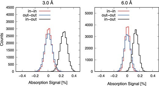
Distribution of absorption signal integrated over the passbands of 3.0 (left) and 6.0 (right) Å around Na D lines. (Color online)
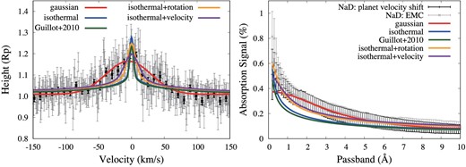
Left: Average values of transmission spectra of Na D lines in velocity space. Our results are indicated in gray and binned by 10 pixels in black. Right: Average absorption of Na D lines. Black is obtained from equation (8) and gray is obtained from |$T_{\rm in{-}out}$|. Both of their errors are estimated from the standard deviation of |$T_\mathrm{out{-}out}$|. The red, blue, green, orange, and navy lines of both figures are the best-fitted spectra using a Gaussian, an isothermal model, an analytic radiative equilibrium model (Guillot 2010), an isothermal model with rotation effect, and an isothermal model with rotation velocity as free parameter. (Color online)
5.2 Comparison with theoretical spectra
The shape of absorption lines is related to the temperature and state of the transmitted atmosphere. We first compare the observed Na absorption line with the theoretical spectra to obtain the relation between temperature and pressure in the atmosphere.
We calculated the theoretical transmission spectra using the model of Kawashima and Ikoma (2018) in basically the same way as done by Fukui et al. (2014, 2016). We calculated the thermochemical equilibrium abundances assuming the solar elemental abundance ratios of Lodders (2003). The thermal ionization of Na was also considered. Line data of Na were taken from Kurucz (1992). We found an appropriate reference radius at 10 bar such that the average transit depth over the wavelength ranges of 5874.89–5886.89 Å and 5898.89–5910.89 Å matched the transit radius measured by Seidel et al. (2019), 2.078 RJ, and the stellar radius revised by Gaia Collaboration (2018), 1.969 R⊙. We have confirmed that the theoretical transmission spectrum calculated with our model can reproduce well that calculated with πη code (Pino et al. 2018), which was the one used by Seidel et al. (2019), when adopting the same parameters.
To explore the atmospheric thermal structure of WASP-76 b from the observed Na absorption line profiles, we considered both isothermal and non-isothermal atmospheres. For the isothermal case, we calculated the model spectra for the temperature range of 1000–5500 K with a grid of 100 K. For the non-isothermal case, we used the analytical model of Guillot (2010) [equation (29) in their paper], which is parameterized with the following five parameters: heat-redistribution factor f, intrinsic temperature Tint, irradiation temperature Tirr, and average opacity in the optical range, kv, and infrared range, kth. We assumed that f = 0.25, which corresponds to the case where the irradiation is effectively redistributed over the entire planetary surface, since we observed the transit. For Tint, given that its effect on the temperature of the upper atmosphere is small, we fixed Tint to be 100 K. For Tirr, we used the value for WASP-76 b (3119 K). For the other two parameters, we varied the values of kth and γ = kv/kth in the ranges of 10−8–1 cm2 g−1 and 10−2–102 with grids of 1 and 0.5 orders of magnitude, respectively.
From comparisons with the isothermal model and an analytic radiative equilibrium model (Guillot 2010), we found that the best fit is achieved with the isothermal model for 3700 K (blue line in figure 12). Nevertheless, the broad width cannot be explained by this model. The rotation of WASP-76 b is about 6.0 km s−1 at the planet radius under the assumption of tidal locking, which is calculated using 2πRp/P. We included the rotation in the theoretical Na D absorption lines and compared them again. The isothermal model for 4200 K (orange line in figure 12) achieved the best fit and had ∼1.1 times lower chi-square than that of the best-fitting isothermal model that did not consider the rotation (table 4). Furthermore, after fitting our data with the isothermal model, in which the rotation velocity was the free parameter, we found that the best-fitting model was the isothermal model for 4300 K with a rotation velocity of ±11 km s−1 (purple line in figure 12).
Chi-square value for each fitting model.*
| Transmission spectrum in velocity space | |||||
| Gaussian | Isothermal | Guillot (2010) | Isothermal and rotation | ||
| 3700 K | kth, γ = 10−7, 101 | 4200 K | |||
| χ2/dof | 247.8|$/$|323 | 332.1|$/$|327 | 341.7|$/$|326 | 292.3|$/$|327 | |
| Reduced-χ2 | 0.77 | 1.02 | 1.05 | 0.90 | |
| Isothermal and velocity | Two-layer | ||||
| 4300 K, ± 11 km s−1 | 3700–2230 K (fixed) | ||||
| χ2/dof | 280.7|$/$|326 | 511.0|$/$|327 | |||
| Reduced-χ2 | 0.86 | 1.56 | |||
| Absorption signal for each passband | |||||
| Gaussian | Isothermal | Guillot (2010) | Isothermal and rotation | ||
| 3700 K | kth, γ = 10−7, 101 | 4200 K | |||
| Fadd | χ2/dof | 6.9|$/$|91 | 120.9|$/$|98 | 164.3|$/$|97 | 37.1|$/$|98 |
| Reduced-χ2 | 0.08 | 1.23 | 1.69 | 0.38 | |
| EMC | χ2/dof | 36.8|$/$|91 | 171.5|$/$|98 | 227.5|$/$|97 | 47.3|$/$|98 |
| Reduced-χ2 | 0.40 | 1.75 | 2.35 | 0.48 | |
| Isothermal and velocity | |||||
| 4300 K, ± 11 km s−1 | 3900 K, ± 0 km s−1 | 5000 K, ± 37 km s−1 | |||
| Fadd | χ2/dof | 30.0|$/$|97 | 87.3|$/$|97 | 129.8|$/$|97 | |
| Reduced-χ2 | 0.31 | 0.90 | 1.33 | ||
| EMC | χ2/dof | 35.8|$/$|97 | 124.0|$/$|97 | 96.6|$/$|97 | |
| Reduced-χ2 | 0.37 | 1.28 | 1.00 | ||
The best-fitting results from our model are shown in bold face. dof = degree of freedom.
We also calculate the absorption for each integral passband for these best-fitting models and compared them with our observation result including the more accurate error obtained with the standard deviation of |$T_{\rm out{-}out}$|. Our observation result is only consistent with the isothermal model considering the spread of velocity. Furthermore, the isothermal models with a velocity with temperatures between 3900 and 5000 K are also consistent with our result in the range of error on the integral passband (right of figure 12; table 4).
These results show that the value of a rotation velocity is necessary to fit both the transmission spectrum and absorption signal like recent studies with HARPS and ESPRESSO (e.g., Seidel et al. 2020b, 2021) but is difficult to estimate without higher accurate observation data and the atmosphere is hotter than the equilibrium temperature (∼2160 K). Its temperature is hotter than the retrieved temperature from the low-resolution spectra obtained with HST, but it is mostly consistent in the upper atmosphere with the model included the near-ultraviolet (NUV) and optical absorption by atoms and molecules such as TiO/VO (see figure 7 in Edwards et al. 2020, figure 2 in Lothringer et al. 2020). However, the temperature in the lower atmosphere is different from that obtained from the low-resolution spectra and the above models. To create the best-fitting model for our data assuming that the temperature in the lower atmosphere (under 10−3 bar) is fixed at the retrieved temperature from low-resolution speca (∼2230 K) , we should consider a model with a higher temperature in the upper atmosphere and with a larger additional velocity, because the absorption lines become sharper and shallower at lower temperatures in the lower atmosphere (figure 13). To identify the T-P profile more clearly, we should combine high-resolution spectroscopy, which is used mainly for observations of the upper atmosphere and low-resolution spectroscopy, and which can be used for observing the lower atmosphere.
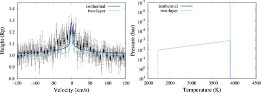
Left: Same as in figure 12 with an isothermal model (blue) and the model with temperature fixed under 10−3 bar (two-layer; light blue). Right: T-P profile for an isothermal model (blue) and a two-layer model (light blue). (Color online)
In addition, to estimate the spread of the line width, we fitted our Na absorption lines by a Gaussian in velocity space (red line in figure 12). The center is blueshifted by about 4.5 km s−1 and the FWHM value is 80.7 ± 7.9 km s−1, which is about 3.0 times broader than that in previous work and about 20 times broader than the sonic speed.
The spread of the width suggests the existence of additional wind (e.g., super-rotation, day-to-night side wind) other than the wind caused by rotation (Seidel et al. 2020b) and time variation, because the observation days in previous work and this work are different. There is also a possibility that there is an instrumental difference. The sodium velocity is up to ∼100 km s−1 considering charge exchange in the sodium exosphere at Jupiter or pickup ions in the Io plasma torus (Gebek & Oza 2020). There is thus a possibility that this spread of the width can be explained by the plasma-driven escape of Na at exo-Io or exo-torus.
Our average transmission spectrum of Na D lines is slightly asymmetric and blueshifted. This supports the day–night chemistry from the detected iron absorption lines with high-resolution spectroscopy (Ehrenreich et al. 2020).
6 Summary
We observed the ultra-hot Jupiter WASP-76 b on 2018 September 10 UT with Subaru/HDS to detect the Na D absorption lines for the atmosphere. The observed data have telluric absorption lines, stellar absorption lines, and an instrumental profile in addition to the absorption lines of the exoplanetary atmosphere. We carefully removed the unnecessary spectra and instrumental profile from the Subaru/HDS data and combined the transmission spectra during transit considering the planet radial velocity.
Na D lines were detected and fitted after correcting for the wide trend around the Na absorption lines with a flat line and two Gaussians. We obtained line contrasts of |$0.42 \pm 0.03\%$| (D1) and |$0.38 \pm 0.04\%$| (D2), FWHM values of 1.63 ± 0.13 Å (D1), and 1.87 ± 0.22 Å (D2), and EWs of (7.29 ± 1.43) × 10−3 Å (D1) and (7.56 ± 2.38) × 10−3 Å (D2). These Na D absorption lines were shallower and broader than those in previous work, but the absorption signals over a given passband are consistent with those in previous work. Our results also show that the spread of the width is 80.7 ± 7.9 km s−1, which is about 3.0 times broader than previous work in velocity space. This result suggests the existence of additional wind. To identify this trend, we should compare our results with a more sophisticated model considering various additional wind patterns, such as that by Seidel et al. (2020b).
In addition, Na D lines were compared with the theoretical transmission spectra calculated based on an isothermal model and an analytic radiative equilibrium model with and without rotation. Isothermal models with temperatures of 3700 K (without rotation) and 4200 K (with rotation) were estimated to have the best fit. These results indicate that the atmospheric temperature is higher than the equilibrium temperature (∼2160 K) and mostly consistent with the temperature in the upper atmosphere estimated by the low-resolution spectral data obtained with HST at NUV, optical, and near-infrared wavelengths. In the future, we will investigate the temperature structure in more detail by combining high- and low-resolution spectra.
Acknowledgements
We would like to thank L. Pino for fruitful discussion and kindly providing us his calculation data for the model comparison, J. V. Seidel for providing observation data, and A. Tajitsu for the support of our Subaru/HDS observation. We also thank MuSCAT team especially M. Mori who teaches how to use the software “emcee”. We are grateful to Forte 〈www.forte-science.co.jp〉 for English editing. This research is based on data collected at Subaru Telescope, which is operated by the National Astronomical Observatory of Japan. We are honored and grateful for the opportunity of observing the Universe from Mauna Kea, which has cultural, historical, and natural significance in Hawaii. Part of our data analysis was carried out on the common use data analysis computer system at the Astronomy Data Center, ADC, of the National Astronomical Observatory of Japan. This work is partly supported by Japan Society for the Promotion of Science (JSPS) KAKENHI Grant Number JP21K13955, JP18H05439, JST PRESTO Grant Number JPMJPR1775, the Astrobiology Center of National Institutes of Natural Sciences (NINS) (Grant Number AB031010). Y.K. is supported by Special Postdoctoral Researcher Program at RIKEN.
Footnotes
IRAF is distributed by the U.S. National Optical Astronomy Observatories, which are operated by the Association of Universities for Research in Astronomy, Inc., under a cooperative agreement with the National Science Foundation.
