


Abstract
We report the first evidence for high-mass star formation triggered by collisions of molecular clouds in M 33. Using the Atacama Large Millimeter/submillimeter Array, we spatially resolved filamentary structures of giant molecular cloud 37 in M 33 using 12CO(J = 2–1), 13CO(J = 2–1), and C18O(J = 2–1) line emission at a spatial resolution of ∼2 pc. There are two individual molecular clouds with a systematic velocity difference of ∼6 km s−1. Three continuum sources representing up to ∼10 high-mass stars with spectral types of B0V–O7.5V are embedded within the densest parts of molecular clouds bright in the C18O(J = 2–1) line emission. The two molecular clouds show a complementary spatial distribution with a spatial displacement of ∼6.2 pc, and show a V-shaped structure in the position–velocity diagram. These observational features traced by CO and its isotopes are consistent with those in high-mass star-forming regions created by cloud–cloud collisions in the Galactic and Magellanic Cloud H ii regions. Our new finding in M 33 indicates that cloud–cloud collision is a promising process for triggering high-mass star formation in the Local Group.
1 Introduction
It is a long-standing question how high-mass stars are formed in galaxies. Three different hypotheses are monolithic collapse, competitive accretion, and stellar mergers (e.g., Zinnecker & Yorke 2007 and references therein). However, these theoretical models have remained controversial due to the lack of conclusive observational evidence.
Recently, the alternative idea of high-mass star formation triggered by “cloud–cloud collisions” has received much attention since the discovery of 50 or more pieces of observational evidence (e.g., Fukui et al. 2018a; Enokiya et al. 2021 and references therein). The colliding clouds have a supersonic velocity difference with an intermediate velocity component—bridging feature—created by the collisional deceleration. The complementary spatial distribution of two clouds (or spatial anti-correlation between the two clouds) is an important signature of collisions because one of the colliding clouds can create a hollowed-out structure in the other cloud. Furthermore, a V-shaped structure can be seen in the position–velocity diagram due to the deceleration and hollowed-out structure. Theoretical studies also support these observational signatures, and predict that cloud–cloud collision increases the effective Jeans mass so high-mass stars can form in the shock-compressed layer (e.g., Habe & Ohta 1992; Anathpindika 2010; Inoue & Fukui 2013; Takahira et al. 2014; Shima et al. 2018; Inoue et al. 2018).
Investigating the universality of the cloud–cloud collision scenario, we need further observational examples in various environments and scales. In the individual Galactic star-forming regions such as Orion and Vela, high-mass star formation can be understood by at least five cloud–cloud collisions on ∼1–100 pc scales (Fukui et al. 2016, 2018a; Fujita et al. 2021c; Sano et al. 2018; Hayashi et al. 2018; Enokiya et al. 2018). It is remarkable that collisions of molecular clouds are seen not only in our Milky Way, but also in the Magellanic Clouds (e.g., Fukui et al. 2015; Saigo et al. 2017). Furthermore, tidally driven galactic-scale (a few kpc scale) collisions of H i clouds are found in the Magellanic and M31–M 33 systems (Fukui et al. 2017, 2019; Tachihara et al. 2018; Tsuge et al. 2019; Tokuda et al. 2019). We can therefore reveal sites of cloud–cloud collisions even in external galaxies if the spatial resolution of CO/H i data is high enough (e.g., a few pc scale).
Here, we report the first evidence for high-mass star formation triggered by collisions of molecular clouds in M 33. Sections 2 and 3 describe the observations and data reduction of the ALMA CO and continuum datasets and their results. Subsection 4.1 gives the properties of high-mass stars in the region; subsection 4.2 discuss the stellar feedback effect, and subsection 4.3 presents a possible scenario of cloud–cloud collision as the formation mechanism of high-mass stars. A summary and conclusions are provided in section 5.
2 Observations and data reduction
We carried out ALMA Band 6 (211–275 GHz) observations toward M 33GMC 37 in Cycle 6 as part of the CO survey toward the supernova remnants in M 33 (PI: H. Sano, #2018.1.00378.S). We used the single-pointing observation mode with 45–49 antennas of the 12 m arrays. The center position of the pointing is (αJ2000.0, δJ2000.0) ∼ (|${01^{\rm h}33^{\rm m}35{_{.}^{\rm s}}9}$|, |${30^{\circ}36^{\prime }27{^{\prime \prime }_{.}}5}$|). The baseline length ranges from 15.06 to 1397.85 m, corresponding to u − v distances from 11.6 to 1074.9 kλ. The maximum recoverable scale (a.k.a. largest angular scale) is calculated to be |${3{^{\prime \prime }_{.}}73}$|. Two quasars, J2253+1608 and J0237+2848, were observed as bandpass and flux calibrators. We also observed the quasar J0112+3208 as a phase calibrator. There were two spectral windows including the 12CO(J = 2–1), 13CO(J = 2–1), and C18O(J = 2–1) line emission with a bandwidth of 117.19 MHz. The frequency resolution was 70.6 kHz for 12CO(J = 2–1), and 141.1 kHz for 13CO(J = 2–1) and C18O(J = 2–1). We also observed two spectral windows as continuum bands, with frequency ranges 231.0–233.0 GHz and 216.3–218.2 GHz. Although these continuum bands contain line emissions of H(30α) and SiO(J = 5–4), we could not detect the two lines significantly.
The data reduction was performed using the Common Astronomy Software Application (CASA; McMullin et al. 2007) package version 5.5.0. We used the “multiscale CLEAN” algorithm implemented in CASA (Cornwell 2008). The synthesized beam of the final dataset is |${0{^{\prime \prime }_{.}}59} \times {0{^{\prime \prime }_{.}}42}$| with a position angle (P.A.) of 0|${_{.}^{\circ}}$|4 for 12CO(J = 2–1), |${0{^{\prime \prime }_{.}}62} \times {0{^{\prime \prime }_{.}}44}$| with a P.A. of 0|${_{.}^{\circ}}$|1 for 13CO(J = 2–1), |${0{^{\prime \prime }_{.}}63} \times {0{^{\prime \prime }_{.}}44}$| with a P.A. of 1|${_{.}^{\circ}}$|1 for C18O(J = 2–1), and |${0{^{\prime \prime }_{.}}59} \times {0{^{\prime \prime }_{.}}43}$| with a P.A. of −1|${_{.}^{\circ}}$|4 for the 1.3 mm continuum. The typical spatial resolution is ∼2 pc at the distance of M 33 (817 ± 59 kpc; Freedman et al. 2001). The typical noise fluctuations of the line emission and continuum are ∼0.15 K at the velocity resolution of 1 km s−1 and 0.017 mJy beam−1, respectively. To estimate the missing flux density, we used the 12CO(J = 2–1) dataset obtained with the IRAM 30 m radio telescope (Gratier et al. 2010; Druard et al. 2014). Following the methods of Druard et al. (2014), we applied a forward efficiency of 0.92 and a main beam efficiency of 0.56 to convert the main beam temperature scale. We compared the integrated intensities of IRAM and ALMA CO data smoothed to match the FWHM resolution of 12″. As a result, we found no significant difference within the error margins, and hence the missing flux density is considered to be negligible.
3 Results
Figure 1a shows an optical composite image of M 33 obtained with the VLT Survey Telescope (VST). The ALMA field of view (FoV) includes several H ii regions located in a spiral arm near the galactic center. Figure 1b shows a large-scale map of ALMA 12CO(J = 2–1) superposed on Hα contours. A giant molecular cloud (GMC)—M 33GMC 37—is mainly located on the western half of the ALMA FoV with filamentary structures. Some of the CO filaments are likely associated with M 33SNR 35, which will be described in a forthcoming paper (H. Sano et al. in preparation). We also note that a bright Hα source with two local peaks at the positions (αJ2000.0, δJ2000.0) ∼ (|${01^{\rm h}33^{\rm m}35{_{.}^{\rm s}}24}$|, |${30^{\circ}36^{\prime }28{^{\prime \prime }_{.}}5}$|) and (|${01^{\rm h}33^{\rm m}35{_{.}^{\rm s}}20}$|, |${30^{\circ}36^{\prime }26{^{\prime \prime }_{.}}5}$|) are superposed on the GMC.
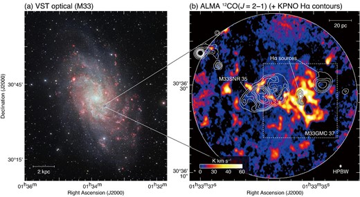
(a) False color image of M 33 obtained with the VLT Survey Telescope (VST, credit: ESO). The red, orange, and cyan represent Hα, r band, and g band, respectively. The blue circle indicates the ALMA FoV. The scale bar is shown in the bottom left corner. (b) Integrated intensity map of 12CO(J = 2–1) obtained with ALMA. The integration velocity range is −145 to −126 km s−1. The superposed white and black contours indicate the Hα intensity obtained by the Kitt Peak National Observatory (KPNO; Massey et al. 2006). The contour levels are 300, 400, 500, 700, 900, 1100, 1500, and 1900 erg s−2 cm−2. The dashed box containing M 33GMC 37 represents the region to be shown in figures 2, 4, 7, and 8. We also show the positions of M 33SNR 35 and Hα sources. The scale bar and beam size are also shown in the top right and bottom right corners, respectively. (Color online)
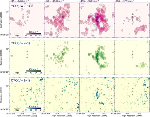
Figures 2a, 2d, and 2g show the maps of moment 0 (integrated intensity) for each line emission toward M 33GMC 37. The area shown in figure 2 is indicated by the dashed box in figure 1. The 12CO(J = 2–1) clouds are detected as diffuse emission with a ring-like structure in the southwest, while the 13CO(J = 2–1) clouds are only bright in the ring-like structure. The C18O(J = 2–1) clouds are concentrated in the central region of the GMC where the 12CO(J = 2–1) and 13CO(J = 2–1) clouds are bright. We also find that there are three sources in the 1.3 mm continuum, as shown in figure 2g′ (GMC 37-MMSs 1–3, hereafter referred to as MMSs 1–3), which are detected at a 5 σ level or higher. The basic physical properties of the three continuum sources are listed in table 1. The peak brightness temperatures of the three sources are comparable, but the spatial extent of MMS 2 is twice as large as for MMSs 1 and 3. It is possible that these millimeter continuum sources are physically related to the Hα emission. In particular, two of them (MMSs 2 and 3) are located in the vicinity of the two Hα peaks (as shown by diamonds in figure 2g′) associated with the brightest CO cloud, indicating that the exciting stars of MMSs 2–3 and Hα peaks are the same. These regions are also bright in the Spitzer 24 μm image (Verley et al. 2007).
![Maps of moment 0 [integrated intensity: (a), (d), and (g)], moment 1 [peak velocity: (b), (e), and (h)], and moment 2 [velocity dispersion: (c), (f), and (i)] toward M 33GMC 35 for each line emission. The contour levels of the moment 0 maps are 8, 14, 22, 32, 44, 58, 74, and 92 K km s−1 for 12CO(J = 2–1); 4, 8, 14, and 22 K km s−1 for 13CO(J = 2–1); and 1, 1.5, 2, 3, and 5 K km s−1 for C18O(J = 2–1). The intensity distribution of the 1.3 mm continuum is also shown in panel (g)′. The contour levels of the millimeter continuum are 9.0, 10.5, and 12.0 × 10⁻² mJy beam−1. The crosses and diamonds represent the intensity peak positions of millimeter continuum sources and Hα. The beam size and scale bar are also shown in the top right and bottom left corners of panels (c), (f), and (i), respectively. (Color online)](https://oup.silverchair-cdn.com/oup/backfile/Content_public/Journal/pasj/73/Supplement_1/10.1093_pasj_psaa045/5/m_psaa045fig2.jpeg?Expires=1749593055&Signature=b5n20Hi0F2k-0xNzlqoziaLqsWGrVb7-abrYDQ~ojwo2e1sbGeMTHE24Du4mJ6i2tcXYzgcjCCVygh4FuBylME8u94izqy19lZj9Ou3uVr0MWGr619bJLp1T2jS5u92XKbUg-36s5dCaem7SP7QBBZIxIwzv46egGBSweUyY0s0WNsgFwmAgZNjWknGLXlJKGazsQGlX4cqZ0fpjjLy1LiqJ~su45tOUsG49JR11A90WRSWZhBnjvRVCG-7qWZY75~lpSpOFkLZKNwVUZSUUkDoftek7R8fVnyPqfAIHF7qorYRogT051Fi2uB0J0vk1KTE~3d7t7hGg0YJPxcXpew__&Key-Pair-Id=APKAIE5G5CRDK6RD3PGA)
Maps of moment 0 [integrated intensity: (a), (d), and (g)], moment 1 [peak velocity: (b), (e), and (h)], and moment 2 [velocity dispersion: (c), (f), and (i)] toward M 33GMC 35 for each line emission. The contour levels of the moment 0 maps are 8, 14, 22, 32, 44, 58, 74, and 92 K km s−1 for 12CO(J = 2–1); 4, 8, 14, and 22 K km s−1 for 13CO(J = 2–1); and 1, 1.5, 2, 3, and 5 K km s−1 for C18O(J = 2–1). The intensity distribution of the 1.3 mm continuum is also shown in panel (g)′. The contour levels of the millimeter continuum are 9.0, 10.5, and 12.0 × 10⁻² mJy beam−1. The crosses and diamonds represent the intensity peak positions of millimeter continuum sources and Hα. The beam size and scale bar are also shown in the top right and bottom left corners of panels (c), (f), and (i), respectively. (Color online)
Physical properties of 1.3 mm continuum sources.*
| Name | αJ2000.0 | δJ2000.0 | Fpeak | Size |
|---|---|---|---|---|
| (h m s) | (° ′ ″) | (mJy beam−1) | (pc) | |
| (1) | (2) | (3) | (4) | (5) |
| GMC 37-MMS 1 | 01 33 35.22 | 30 36 29.0 | 0.12 | 1.7 |
| GMC 37-MMS 2 | 01 33 35.22 | 30 36 27.8 | 0.13 | 3.0 |
| GMC 37-MMS 3 | 01 33 35.22 | 30 36 26.4 | 0.11 | 1.6 |
*Column (1): Name of millimeter continuum source. Columns (2)–(3): Positions of the maximum flux. Column (4): Peak flux of 1.3 mm continuum. Column (5): Size of continuum source defined as (S/π)0.5 × 2, where S is the total surface area of the continuum source surrounded by a contour of the 5 σ level.
Figures 2b, 2e, and 2h show the maps of moment 1 (peak velocity). The peak velocities of the 12CO(J = 2–1) and 13CO(J = 2–1) clouds are discontinuous, with a velocity jump of ∼10 km s−1 toward the millimeter continuum sources and their eastern side, while that of the C18O(J = 2–1) line emission shows no significant velocity jump within the clouds. Figures 2c, 2f, and 2i show the maps of moment 2 (velocity dispersion). A larger velocity dispersion above 3 km s−1 is seen in several regions of both the 12CO(J = 2–1) and 13CO(J = 2–1) clouds, where the velocity jumps are identified (see also figure 2b). On the other hand, there is no sign of such larger velocity dispersion in the C18O(J = 2–1) clouds.
Figure 3 shows the typical CO spectra toward three positions, A, B, and C. Position A represents the direction of MMS 1. Positions B and C correspond to the regions with the largest velocity dispersion in the 13CO(J = 2–1) line emission (see also figure 2f) and the maximum intensity of the C18O(J = 2–1) line emission (see also figure 2g), respectively. The CO spectra of position A is centered at ∼132 km s−1, corresponding to the systemic velocity of the M 33GMC 37 region which was derived by a rotation model of the H i disk (Gratier et al. 2010). We note that the 12CO(J = 2–1) line emission shows a wing-like profile with a velocity extent of more than 5 km s−1. For position B, we find double-peak profiles in both the 12CO(J = 2–1) and 13CO(J = 2–1) line emissions, suggesting that there are two individual clouds toward the line of sight. We hereafter refer to the component at VLSR = −143.0 to −134.0 km s−1 as the “blue cloud” and that at VLSR = −133.0 to −127.0 km s−1 as the “red cloud.” On the other hand, the CO spectra of position C—the brightest peak in C18O(J = 2–1)—show a single-peak profile for each line emission. Note that their central velocities of VLSR ∼ −133.5 km s−1 roughly correspond to the mean velocity of the red and blue clouds.
![Typical CO spectra for the positions A [$(\alpha _\mathrm{J2000.0}, \delta _\mathrm{J2000.0}) = ({01^{\rm h}33^{\rm m}35{_{.}^{\rm s}}22}, {30^{\circ}36^{\prime }29{^{\prime \prime }_{.}}5})$], B [$(\alpha _\mathrm{J2000.0}, \delta _\mathrm{J2000.0}) = ({01^{\rm h}33^{\rm m}35{_{.}^{\rm s}}19}, {30^{\circ}36^{\prime }27{^{\prime \prime }_{.}}5})$], and C [$(\alpha _\mathrm{J2000.0}, \delta _\mathrm{J2000.0}) = ({01^{\rm h}33^{\rm m}35{_{.}^{\rm s}}25}, {30^{\circ}36^{\prime }26{^{\prime \prime }_{.}}5})$].](https://oup.silverchair-cdn.com/oup/backfile/Content_public/Journal/pasj/73/Supplement_1/10.1093_pasj_psaa045/5/m_psaa045fig3.jpeg?Expires=1749593055&Signature=vSwrOIgEyO4efD1tmyVczjmgkwDjTFRpVZOi15lSqs0cT8tA6ZxwL24Qy0~5efsFTi-mfE8bDZpapMREmzDYL3q4gLBLCrx6fH8EOfmXPzXhX6Dhy3Mt9CsOnmQu1sE4JVEoSfDlWKna-WorFYjHfqbogEiF1Jna3QfGDUTzljtCSFefj5nR-8jA1rhoogkNcAFagQHbZeGfXPtPJLmNoNxcNLV4a547LcncEwKp2PaxED2u4~gsf-GdaRUI6K572HcyWBw2lXE3dy7iyDOlH2lBe40L4TVeTNB8UzAS6WrRgENewyHJOEG5uy~KwuK0d1d6Nu~NJTf7w3dkLhvHDQ__&Key-Pair-Id=APKAIE5G5CRDK6RD3PGA)
Typical CO spectra for the positions A [|$(\alpha _\mathrm{J2000.0}, \delta _\mathrm{J2000.0}) = ({01^{\rm h}33^{\rm m}35{_{.}^{\rm s}}22}, {30^{\circ}36^{\prime }29{^{\prime \prime }_{.}}5})$|], B [|$(\alpha _\mathrm{J2000.0}, \delta _\mathrm{J2000.0}) = ({01^{\rm h}33^{\rm m}35{_{.}^{\rm s}}19}, {30^{\circ}36^{\prime }27{^{\prime \prime }_{.}}5})$|], and C [|$(\alpha _\mathrm{J2000.0}, \delta _\mathrm{J2000.0}) = ({01^{\rm h}33^{\rm m}35{_{.}^{\rm s}}25}, {30^{\circ}36^{\prime }26{^{\prime \prime }_{.}}5})$|].
The 13CO(J = 2–1) and C18O(J = 2–1) brightness temperatures are multiplied by a factor of two and five, respectively. The vertical dashed line indicates the systemic velocity of M 33GMC 37. (Color online)
Figures 4a and 4b show the spatial distributions of the blue and red clouds. The blue cloud is elongated in the northwestern direction, while the red cloud is stretched in the southwestern direction. Both clouds have filamentary CO structures. The typical width and length of filaments are ∼3 pc and ∼10 pc, respectively. The total mass is estimated to be ∼2.4 × 10⁵ M⊙ for the blue cloud and ∼1.9 × 10⁵ M⊙ for the red cloud using equations (1) and (2). Note that MMS 2 is likely associated not only with the brightest peak of the blue cloud, but also with that of the red cloud. The other continuum sources—MMSs 1 and 3—appear to be overlapped with both the red and blue clouds. The peak column density of molecular hydrogen is ∼4.5 × 1022 cm−2 for the blue cloud, and ∼4.1 × 1022 cm−2 for the red cloud. We also find a small hole-like structure in the blue cloud centered at (αJ2000.0, δJ2000.0) ∼ (|${01^{\rm h}35^{\rm m}35{_{.}^{\rm s}}28}$|, |${30^{\circ}36^{\prime }27{^{\prime \prime }_{.}}5}$|). Note that the peak positions of Hα and the millimeter continuum are placed on the edge of the hole-like structure, not on the center of it.
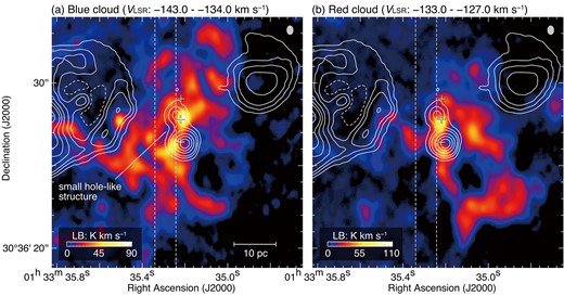
Integrated intensity maps of 12CO(J = 2–1). The velocity range is −143 to −134 km s−1 for panel (a) and −133 to −127 km s−1 for panel (b). The vertical dashed lines indicate the integration range in RA for figure 5. The crosses represent the positions of the 1.3 mm continuum. The white contours indicate Hα emission as shown in figure 1b. The scale bar and beam size are also shown in the bottom and top right corners for each panel. (Color online)
Figure 5 shows the position–velocity diagram of 12CO(J = 2–1). The integration range in right ascension is from |${01^{\rm h}33^{\rm m}35{_{.}^{\rm s}}243}$| to |${01^{\rm h}33^{\rm m}35{_{.}^{\rm s}}341}$|, corresponding to the spatial extent of the small hole-like structure appearing in the blue cloud (see also figure 4a). The blue cloud is clearly seen; its radial velocity is centered at VLSR ∼ −137 km s−1. We find a V-shaped structure in the position–velocity diagram (see the dashed black lines in figure 5). The center velocity of the red cloud (VLSR ∼ −132 km s−1) corresponds to the vertex of the V-shaped structure. The cavity-like structure and intensity peak of 12CO(J = 2–1) are seen at (δJ2000.0, VLSR) ∼ (|${30^{\circ}36^{\prime }27{^{\prime \prime }_{.}}5}$|, −135.0 km s−1) and (|${30^{\circ}36^{\prime }26{^{\prime \prime }_{.}}5}$|, −134.0 km s−1), respectively.
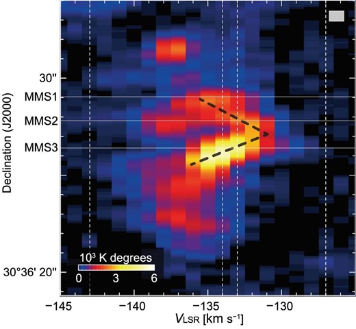
Declination–velocity diagram of 12CO(J = 2–1). The integration range is from |${01^{\rm h}33^{\rm m}35{_{.}^{\rm s}}243}$| to |${01^{\rm h}33^{\rm m}35{_{.}^{\rm s}}341}$|. The vertical lines indicate the integration velocity ranges for figure 4. The three horizontal solid lines indicate the declination positions of MMSs 1–3. The beam size is shown in the top right corner. (Color online)
4 Discussion
4.1 Presence of high-mass stars and their spectral types
Although there is no previous study of the stars embedded within the H ii region in M 33, the detection of bright Hα emission, the 1.3 mm continuum sources MMSs 1–3, and 24 μm emission indicates that several high-mass stars are associated with the two molecular clouds. To confirm the presence of high-mass stars, we compared them with archival optical datasets obtained with the Hubble Space Telescope (HST). Figure 6 shows the high spatial resolution optical images obtained with the HST WFPC2 and WFC3 detectors. The coordinate offsets of all datasets obtained with HST were corrected by comparing the position of the bright point sources with those catalogued in Gaia Data Release 2 (Gaia Collaboration 2018). We can clearly see ∼10 high-mass stars bright in the U band, Hα, and IR band within the Kitt Peak National Observatory (KPNO) Hα contours. Hereafter, we assume that ten high-mass stars are associated with the Hα, 1.3 mm continuum sources, and 24 μm emission.
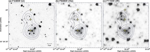
Maps of optical images obtained with the Hubble Space Telescope (HST): (a) HST/WFC3 map with F336W filter (U band), (b) HST/WFPC2 map with F606W filter (Hα), and (c) HST/WFC3 map with F110W filter (IR). The superposed contours and crosses are the same as in figure 4. The scale bar is also shown in the bottom right corner in panel (a).
4.2 Can stellar feedback explain the large velocity separation of the two clouds?
In the present study, we spatially resolved filamentary CO structures of M 33GMC 37 using ALMA with a spatial resolution of ∼2 pc (|$\Delta \theta \sim {0{^{\prime \prime }_{.}}5}$|). There are two individual molecular clouds, red and blue, with a velocity separation of ∼6 km s−1 and a mass of ∼2 × 10⁵ M⊙ for each. The densest part of the GMC is significantly detected in C18O(J = 2–1), containing up to ∼10 high-mass stars with spectral types B0V–O7.5V. In this section, we shall discuss whether the velocity separation of the two clouds can be explained by acceleration due to stellar feedback.
First, we claim that the total momentum of the stellar winds is significantly lower than that of the two molecular clouds. The typical wind momentum of an O-type star is calculated to be ∼2 × 10³ M⊙ km s−1, by considering a mass accretion rate of ∼10−6 M⊙ yr−1, a wind duration time of ∼106 yr, and a wind velocity of ∼2000 km s−1 (see Kudritzki & Puls 2000 and references therein). In the case of M 33GMC 37, the total wind momentum is therefore ∼2 × 10⁴ M⊙ km s−1, assuming that there are ten O-type stars (see subsection 4.1). On the other hand, we derive a total cloud momentum of ∼1.3 × 10⁶ M⊙ km s−1. Here we assume that the two clouds show an expanding motion with an expansion velocity of ∼3 km s−1, corresponding to half the value of the velocity separation of the two clouds. Since the total cloud momentum is roughly two orders of magnitude higher than the total wind momentum, we conclude that the velocity separation of the two clouds cannot be explained by expanding gas motion due to stellar feedback.
This interpretation is also consistent with the velocity distributions of the two clouds. If the expansion of the clouds is centered at an exciting star, a ring-like gas distribution would be expected not only in the spatial distribution such as the moment 0 map, but also in the position–velocity diagram (cf. figure 8 in Torii et al. 2015). For M 33GMC 37, however, we could not find such distributions around the 3 mm continuum sources (see figures 3 a and 5). We have also created velocity channel maps in order to justify the velocity and spatial distributions of the clouds, because expanding clouds will be spatially shifted from inward to outward in the velocity channel maps (e.g., Fukui et al. 2012; Sano et al. 2017b). Figure 7 shows the velocity channel maps for each CO line emission. We confirmed that there are no clear signs of such spatial shifts with increasing velocity. On the other hand, we note that a tiny CO clump near MMS 2 appears in all velocity ranges of the 12CO(J = 2–1) line emission, suggesting possible evidence of outflowing gas in addition to the wing-like profile of MMS 1 (figure 2a). Although the outflowing gas candidate is very concentrated, within 1 pc scales, the outflowing gas could not strongly affect the dynamical motion of the two clouds. To summarize, the stellar feedback effect is negligible for the cloud kinematics, and therefore the velocity separation of the two clouds cannot be explained by acceleration by stellar winds and outflowing gas.
Velocity channel maps of (a) 12CO(J = 2–1), (b) 13CO(J = 2–1), and (c) C18O(J = 2–1) line emission toward M 33GMC 37. Each panel shows the intensity distribution integrated every 5 km s−1 in a velocity range from −145 to −125 km s−1. The contour levels are 4, 8, 14, 22, 32, 44, 58, and 74 K km s−1 for 12CO(J = 2–1); 2, 4, 8, and 14 K km s−1 for 13CO(J = 2–1); and 1.5, 2, 3, and 5 K km s−1 for C18O(J = 2–1). The beam size and scale bar are also shown in the top right and bottom left corner, respectively. The crosses indicate the positions of the millimeter continuum sources. (Color online)
4.3 An alternative idea: High-mass star formation triggered by cloud–cloud collisions in M 33GMC 37
In the previous section we concluded that the velocity separation of the two clouds is not caused by the stellar feedback effect. It is therefore reasonable to assume that the two individual clouds have collided with each other and have formed the high-mass stars embedded within M 33GMC 37. In this section we discuss this second scenario.
To form high-mass stars via cloud–cloud collisions, a supersonic velocity separation of the two colliding clouds is essential. According to magnetohydrodynamical numerical simulations, the effective Jeans mass in the shock-compressed layer is proportional to the third power of the effective sound speed (Inoue & Fukui 2013). Here, the effective sound speed is defined as |$\langle c_\mathrm{s}^2 + c_\mathrm{A}^2 + \Delta v^2 \rangle ^{0.5}$|, where cs is the sound speed, cA is the Alfvén speed, and Δv is the velocity dispersion. A supersonic velocity separation of at least a few km s−1 therefore produces a large mass accretion rate, on the order of ∼10−4–10−3 M⊙ yr−1, which allows mass growth of stars against the stellar feedback (Inoue & Fukui 2013). For the case of M 33GMC 37, the observed velocity separation of the red and blue clouds is ∼6 km s−1 (see the CO spectra in figure 2b). Although the velocity separation will be changed due to the projection effect, this is roughly consistent with the typical velocity separation in the Galactic high-mass star-forming regions triggered by cloud–cloud collisions: e.g., M 20 (∼7.5 km s−1, Torii et al. 2011), RCW 36 (∼5 km s−1, Sano et al. 2018), M 42 (∼7 km s−1, Fukui et al. 2018a), and RCW 166 (∼5 km s−1, Ohama et al. 2018).
We next focus on the velocity structures of the two colliding clouds. Previous numerical simulations and observational results have demonstrated that colliding clouds create an intermediate velocity component—bridging feature—connecting two clouds due to the deceleration by collisions, if the projected velocity separation is significantly larger than the linewidth of the colliding clouds (see Fukui et al. 2018a and references therein). When the two colliding clouds have roughly the same column density of gas, the two clouds will be merged and appear as a single-peak CO profile centered at the mean velocity of the two colliding clouds (e.g., Fukui et al. 2017). In the case of M 33GMC 37, the VLSR ∼ −135 km s−1 feature in the 13CO spectrum at position A is possibly a bridging feature (see figure 2b), but is not significantly detected because of the small velocity separation of the two colliding clouds. However, the CO spectra at position B—the densest part of the colliding clouds—show single-peak CO profiles centered at VLSR ∼ −133.5 km s−1, roughly corresponding to the mean velocity of the red and blue clouds (see also figure 2c). This is consistent with the two clouds having roughly the same column density of ∼4–5 × 1022 cm−2, assuming cloud–cloud collision has occurred.
The V-shaped structure in the position–velocity diagram as shown in figure 5 provides us with suggestive evidence for head-on cloud–cloud collision. As discussed above, an intensity depression or a hole-like structure might indicate the spot of collision between two clouds for the case of a head-on collision. If we make a position–velocity diagram that includes the collision region, we can find not only the bridging feature but also the V-shaped structure (e.g., Fukui et al. 2018a, 2018c, 2018d; Hayashi et al. 2018; Torii et al. 2018, 2021; Fujita et al. 2019b). Note that if an oblique collision—e.g., collisions with the edges of the clouds—occurred, we could not find such a V-shaped structure in the position–velocity diagram (Fujita et al. 2021c). For M 33GMC 37, we can clearly see the V-shaped structure connecting the red and blue clouds as the intermediate velocity component that is called the bridging feature. Moreover, the presence of an intensity peak and depression in the V-shaped structure is predicted by synthetic observations of a theoretical result of a head-on cloud–cloud collision (e.g., Fukui et al. 2018c).
Another important signature of a collision is complementary spatial distribution of the colliding clouds. In general, colliding clouds are not the same size, such as simulated by Habe and Ohta (1992) and Anathpindika (2010). In fact, observational results indicate that colliding clouds have different sizes, morphologies, and density distributions (e.g., Hasegawa et al. 1994; Furukawa et al. 2009; Fukui et al. 2014, 2018a, 2018b; Enokiya et al. 2018; Tokuda et al. 2018; Dewangan et al. 2019a, 2019b). In such cases, one of the colliding clouds can create a hole-like structure in the other cloud, if the colliding cloud has a denser part and/or smaller size than the other cloud. This produces a complementary spatial distribution of two clouds with different systematic velocity. Furthermore, the angle of the two colliding clouds θ is generally not 0° or 90° relative to the line of sight. This means that we can also observe a spatial displacement between the complementary distributions of two clouds.
To evaluate such complementary distributions of two colliding clouds, it is useful to calculate the correlation coefficient between the intensity distributions of the two clouds (cf. Fujita et al. 2021b). If the correlation coefficient between the two colliding clouds shows a negative value, the two clouds show complementary spatial distributions. The lower the correlation coefficient, the higher the complementarity. By changing the values of the spatial displacement for one of the colliding clouds, we can obtain a map of the correlation coefficient between the two clouds as a function of displacement. The best-fitting value of the displacement for each coordinate can be derived as the point of local minimum.
In M 33GMC 37, we find complementary spatial distributions of the red and blue clouds by following the above method. Figure 8a shows the map of the blue cloud superposed on the red cloud contours with a spatial displacement of ∼6.2 pc toward the southeast direction. The brightest peak of the red cloud fits within the hole-like structure of the blue cloud. The second and third minor peaks of the red cloud also show good complementary distributions (or anti-correlation) with the blue cloud. Figure 8b shows the map of the correlation coefficient between the two clouds as a function of the spatial displacement of the red cloud in the directions of right ascension and declination. Since the cloud collision in M 33GMC 37 is likely a head-on collision, the correlation coefficients were calculated toward the inner parts of the blue cloud. We can find the local minimum with a correlation coefficient of −0.44 at a shift by 15 pix in RA and −12 pix in Dec, which is significantly lower than the correlation coefficient of −0.05 without displacement. We also calculate a p-value which provides information about whether a statistical hypothesis is significant or not. As a result, the correlation coefficient of −0.44 is significant at the 0.5% significance level.
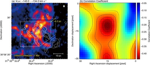
(a) Complementary spatial distribution of the red (contours) and blue clouds (image). The velocity ranges of image and contours are the same as shown in figures 4a and 4b, respectively. The contour levels are 16, 26, 36, 46, 56, and 66 K km s−1. The contours are spatially displaced ∼6.2 pc in the southeast direction (P.A. = 137°). The dashed and solid rectangles indicate the before and after displacement of the contours, respectively. The crosses and diamonds are the same as shown in figure 2. The scale bar and beam size are also shown in the bottom and top right corner, respectively. (b) Map of Pearson’s correlation coefficient as a function of displacements in the right ascension direction and in the declination direction in pixel units. The size of a pixel is 84.5 mas. The coordinate origin is (αJ2000.0, |$\delta _\mathrm{J2000.0}) = ({01^{\rm h}33^{\rm m}35{_{.}^{\rm s}}22}, {30^{\circ}36^{\prime }27{^{\prime \prime }_{.}}5})$|. The intensity distributions of 12CO(J = 2–1) enclosed by the dashed polygon (blue cloud) and the solid polygon (red cloud) were used to calculate the correlation coefficient. The superposed contours indicate the values of the correlation coefficients, whose levels are −0.435, −0.430, −0.415, −0.390, −0.355, and −0.310. (Color online)
If the cloud collision scenario is correct, we can also estimate the collision time scale as a dynamical time scale using the values of the displacement and velocity difference of the two clouds of (spatial displacement)|$/$|(velocity difference) = 8.8 pc|$/$|8.5 km s−1 ∼1 Myr, assuming a collision angle of θ = 45°. Since GMCs are thought to be dispersed within ∼1.5 Myr due to strong stellar winds and UV radiation (Kruijssen et al. 2019), the shorter collision time scale is consistent with the presence of dense molecular clouds surrounding the high-mass stars and small H ii regions with a few pc extent in Hα emission because of the young age of the high-mass stars (see figures 1b and 4).
We also note that the number of high-mass stars (≲ 10) in M 33GMC 37 is consistent with previous observational studies of cloud–cloud collisions. According to Fukui et al. (2018a), the formation of super star clusters containing more than ten O-type stars requires collisions of two dense clouds, one of which has a high column density of at least ∼1023 cm−2 (e.g., RCW 38, Fukui et al. 2016; NGC 3603, Fukui et al. 2014; Westerlund 2, Furukawa et al. 2009). On the other hand, the formation of single or a few O-type stars happens in a collision between molecular clouds with low column density of several 1022 cm−2 or less (e.g., RCW 120, Torii et al. 2015; NGC 2359, Sano et al. 2017a; S44, Kohno et al. 2021; N4, Fujita et al. 2019; more detailed results are summarized in Enokiya et al. 2021). For M 33GMC 37, the two colliding clouds have a low column density of ∼4–5 × 1022 cm−2. Therefore, cloud–cloud collisions in M 33GMC 37 can create ∼10 high-mass stars at most. This is consistent with ∼10 stars being detected by HST optical images within the KPNO Hα boundary (see figure 6).
In addition, Enokiya, Torii, and Fukui (2021) recently revealed that the number of OB stars formed in cloud collisions depends not only on the column density, but also on the velocity difference of the two colliding clouds. Figure 9 shows a correlation plot between the column density and relative velocity toward the sites of cloud–cloud collisions in the Milky Way (Enokiya et al. 2021). The authors found that too fast or slow cloud collisions cannot form OB stars even if the cloud column density is high enough. In the case of M 33GMC 37, the observational parameters are consistent with the trend seen in previous studies. This possibly indicates that there is no critical difference between the Milky Way and M 33 from the point of view of high-mass star formation triggered by cloud–cloud collisions. To evaluate the interpretation, more evidence on high-mass star formation triggered via cloud–cloud collisions is needed. Future ALMA observations of young massive clusters in M 33 will allow us to study the detailed processes of high-mass star formation.
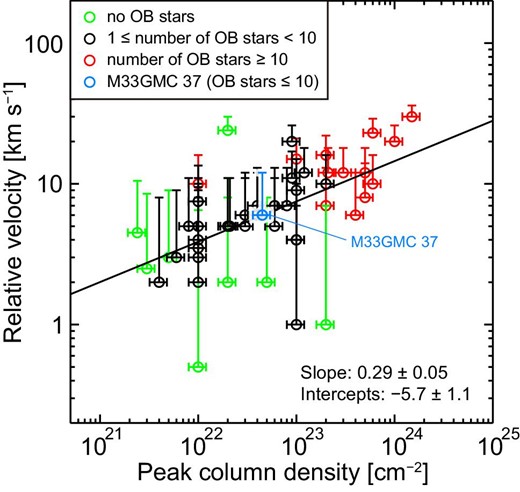
Scatterplot between the peak column density of molecular hydrogen and the relative velocity of two colliding clouds toward sites of cloud–cloud collisions in the Milky Way (Enokiya et al. 2021). The green, black, and red circles represent the H ii regions associated with no OB stars, fewer than ten OB stars, and more than ten OB stars, respectively. The solid line indicates the regression line obtained by least-squares fitting (Enokiya et al. 2021). We also added the data point of M 33GMC 37 as the cyan circle. (Color online)
Finally, we present a summary picture of the high-mass star formation triggered by the cloud collisions in M 33GMC 37. Figure 10 shows schematic images of the cloud–cloud collisions in M 33GMC 37. First, the red and blue clouds were moving in the direction approaching each other with a relative velocity of more than 6 km s−1 with respect to the line of sight. Next, the two clouds collided with each other ∼1 Myr ago. The continuous collisions created the complementary spatial distributions between the two clouds (figures 10a and 8a). The molecular gas was efficiently compressed, especially in the dense collision layers, which formed the high-mass stars toward MMSs 2 and 3 (yellow crosses). Finally, the red cloud penetrated the blue cloud, making the small hole-like structure, and moved behind the blue cloud, which corresponds to the present positions of the two clouds (figures 10b and 4). The high-mass star in MMS 1 might have formed recently when the edge of the red cloud finally reached the position of MMS 1. The bright spot and cavity structure in the position–velocity diagram are also consistent with the positions of the dense collision layers and the hole-like structure in the blue cloud, respectively (figure 5).
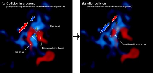
Schematic images of the cloud–cloud collisions in M 33GMC 37 for the phases of (a) collision in progress and (b) after collision. The red and blue colors represent the red and blue clouds, respectively. The red and blue arrows indicate the directions of movement of the red and blue clouds, respectively. The dense collision layers and the small hole-like structure in the blue cloud are also indicated. The yellow crosses indicate the positions of MMSs 1–3. (Color online)
To summarize, the red and blue clouds in M 33GMC 37 fulfill four requirements of high-mass star formation triggered by cloud–cloud collisions, as follows: (1) supersonic velocity separation of the two clouds, (2) complementary spatial distribution with the displacement of the colliding clouds, (3) the presence of a bridging feature connecting the two clouds in velocity space, and (4) a V-shaped structure in the position–velocity diagram. We therefore suggest that the high-mass stars corresponding to ten B0V–O7.5V types in M 33GMC 37 were formed by cloud–cloud collisions. Further ALMA observations of M 33 GMCs will allow us to study high-mass star formation via cloud–cloud collisions in the spiral galaxy, the results of which can be directly compared with the Milky Way and Magellanic Clouds.
5 Conclusion
In the present study, we carried out new CO(J = 2–1) and continuum observations of M 33GMC 37 using ALMA with an angular resolution of ∼|${0{^{\prime \prime }_{.}}5}$|, corresponding to a spatial resolution of ∼2 pc at the distance of M 33. We revealed two individual molecular clouds with a velocity separation of ∼6 km s−1 that are associated with up to ∼10 high-mass stars of spectral types B0V–O7.5V. The two molecular clouds show complementary spatial distribution with a spatial displacement of ∼6.2 pc. An intermediate velocity component of the two clouds as a V-shaped structure in the position–velocity diagram was also detected. We proposed a possible scenario whereby the high-mass stars in M 33GMC 37 were formed by cloud–cloud collisions approximately 1 Myr ago.
Acknowledgements
This paper makes use of the following ALMA data: ADS/JAO ALMA#2018.1.00378.S. ALMA is a partnership of ESO (representing its member states), NSF (USA), and NINS (Japan), together with NRC (Canada), NSC and ASIAA (Taiwan), and KASI (Republic of Korea), in cooperation with the Republic of Chile. The Joint ALMA Observatory is operated by ESO, AUI/NRAO, and NAOJ. Based on observations made with the NASA/ESA Hubble Space Telescope, and obtained from the Hubble Legacy Archive, which is a collaboration between the Space Telescope Science Institute (STScI/NASA), the Space Telescope European Coordinating Facility (ST-ECF/ESA), and the Canadian Astronomy Data Centre (CADC/NRC/CSA). This study was financially supported by Grants-in-Aid for Scientific Research (KAKENHI) of the Japanese Society for the Promotion of Science (JSPS, grant nos. 16K17664, 18J01417, and 19K14758). K. Tokuda was supported by NAOJ ALMA Scientific Research Grant Number 2016-03B. H.S. was also supported by the ALMA Japan Research Grant of NAOJ Chile Observatory (grant no. NAOJ-ALMA-226). M.S. acknowledges support by the Deutsche Forschungsgemeinschaft through the Heisenberg professor grants SA 2131/5-1 and 12-1. We are also grateful to the anonymous referee for useful comments which helped the authors to improve the paper.
