


Abstract
A supersonic cloud–cloud collision produces a shock-compressed layer which leads to formation of high-mass stars via gravitational instability. We carried out a detailed analysis of the layer by using the numerical simulations of magneto-hydrodynamics which deal with colliding molecular flows at a relative velocity of 20 km s−1 (Inoue & Fukui 2013, ApJ, 774, L31). Maximum density in the layer increases from 1000 cm−3 to more than 105 cm−3 within 0.3 Myr by compression, and the turbulence and the magnetic field in the layer are amplified by a factor of ∼5, increasing the mass accretion rate by two orders of magnitude to more than 10−4 |$ M_{\odot } $| yr−1. The layer becomes highly filamentary due to gas flows along the magnetic field lines, and dense cores are formed in the filaments. The massive dense cores have size and mass of 0.03–0.08 pc and 8–|$ 50\, M_{\odot } $| and they are usually gravitationally unstable. The mass function of the dense cores is significantly top-heavy as compared with the universal initial mass function, indicating that the cloud–cloud collision preferentially triggers the formation of O and early B stars. We argue that the cloud–cloud collision is a versatile mechanism which creates a variety of stellar clusters from a single O star like RCW 120 and M 20 to tens of O stars of a super star cluster like RCW 38 and a mini-starburst W 43. The core mass function predicted by the present model is consistent with the massive dense cores obtained by recent ALMA observations in RCW 38 (Torii et al. 2021, PASJ, in press) and W 43 (Motte et al. 2018, Nature Astron., 2, 478). Considering the increasing evidence for collision-triggered high-mass star formation, we argue that cloud–cloud collision is a major mechanism of high-mass star formation.
1 Introduction
Formation of high-mass stars has been an issue of compelling interest in the last two decades because the influence of high-mass stars in galactic evolution is overwhelming and profound. Considerable efforts have been paid toward understanding high-mass star formation by a number of papers (Tan et al. 2014; Krumholz 2015).
Three scenarios have been considered until now in the literature. They are (1) stellar collisions in a rich stellar cluster (Bonnell et al. 1998), (2) the competitive accretion in a massive self-gravitating system (Bonnell et al. 2001), and (3) the monolithic collapse of a dense cloud (McKee & Tan 2002; Krumholz et al. 2009). If the stellar density is high enough for frequent collision between stars, collisional merging of low-mass stars may work as a possible mechanism. Later, it was proved that the stellar density has to be uncomfortably large for such collisions to be efficient, and stellar collisions are no longer considered as a viable mechanism of high-mass star formation (Moeckel & Clarke 2011). The other two mechanisms remain to be confronted by observations, and it is not yet settled how high-mass stars are forming (see for a review Tan et al. 2014). A possible argument unfavorable to the competitive accretion is an isolated O star such as the exciting star of M 20 and RCW 120, which does not belong to a massive cluster (Torii et al. 2011, 2015; see also Ascenso 2018). The numerical simulations of the monolithic collapse by Krumholz et al. (2009) showed the formation of O stars from molecular gas of |$100\, M_{\odot }$| confined within 0.1 pc. This initial condition was adopted from observations of a protostar candidate IRAS 05358+3543 in the S233–235 high-mass-star-forming region and other typical regions of high-mass star formation (Beuther et al. 2007; see also McKee & Tan 2002). A recent analysis of molecular gas by R. Yamada et al. (in preparation) showed that IRAS 05358+3543 was possibly formed by an external trigger of a cloud–cloud collision, an ad-hoc, externally driven situation, raising caution around the initial condition adopted by Krumholz et al. (2009).
High-mass star formation requires accumulating large cloud mass into a small volume. Suppose that the initial condition is a massive low-density cloud and the final phase is a small dense cloud of the same mass which rapidly forms high-mass star(s). This scenario requires an intermediate phase when cloud density is high enough to form low-mass stars, unless the phase has a time scale much shorter than the free-fall time scale. During the phase, star formation has to be strongly suppressed; otherwise the cloud loses mass by star formation before being collected into the small volume and high-mass star(s) cannot be formed. Such a naive thought may be useful to shed light on the essence of the high-mass star formation as suggested in a review article by Zinnecker and Yorke (2007, section 9):
while no further pursuits on “the rapid external compression” are found in the literature.“Rapid external shock compression (i.e., supersonic gas motions) generating high column densities in less than a local free-fall time rather than slow quasistatic build-up of massive cores may be the recipe to set up the initial conditions for local and global bursts of massive star formation”
Cloud–cloud collision is another promising mechanism of the high-mass star formation as shown by recent theoretical and observational works, and has become a possible alternative to the previous scenarios (2) and (3) of high-mass star formation given above. Habe and Ohta (1992) showed that, in a supersonic collision between small and large molecular clouds, the small cloud creates a cavity in the large cloud, and the layer between the two clouds is strongly compressed to higher density, where a condition favorable for high-mass star formation is realized (Habe & Ohta 1992; Anathpindika 2010; Takahira et al. 2014; Shima et al. 2018). After the onset of the collision, the two clouds show complementary distribution between the cavity and the small cloud, and the interface layer shows a broad bridge feature connecting the two clouds in velocity (Haworth et al. 2015). Recent observations show that in more than 50 regions of high-mass star formation these observational signatures of collision are identified and typical cloud properties are derived, such as density and mass of the colliding clouds (Enokiya et al. 2021). These objects includes H ii regions and super star clusters in the Milky Way and the Local Group (e.g., M 42/M 43, Fukui et al. 2018a; M 17, Nishimura et al. 2018; NGC 6334 and NGC 6357, Fukui et al. 2018b; M 20, Torii et al. 2011, 2017; RCW 120, Torii et al. 2015; RCW 38, Fukui et al. 2016; Westerlund 2, Furukawa et al. 2009; Ohama et al. 2010; NGC 3603, Fukui et al. 2014; R136, Fukui et al. 2017).
It is important to understand the detailed properties of the forming stars under a trigger of a cloud–cloud collision, and theoretical understanding of the physical properties of the colliding clouds is crucial. Magneto-hydrodynamic (MHD) numerical simulations were made for molecular gas flows colliding supersonically in a plane-parallel configuration by Inoue and Fukui (2013), and they showed that dense cores around |$100\, M_{\odot }$|, precursors of high-mass stars, are formed. These simulations also showed that the layer is characterized by enhanced turbulence and magnetic field where the effective sound velocity is increased by several times depending on the collision velocity. As a result, the mass accretion rate, which is proportional to the third power of the effective sound speed, becomes as high as 10−4–|$10^{-3}\, M_{\odot }\:$|yr−1, which satisfies a value high enough to overcome the stellar radiation feedback (Wolfire & Cassinelli 1987). Since the simulations include more details of the compressed layer such as the mass function of the dense cores, which were not presented by Inoue and Fukui (2013), it is worthwhile to explore the molecular gas properties in the simulations further. Such a study will shed light on the time evolution in a cloud–cloud collision and help us to obtain an insight into the triggered high-mass star formation.
The aim of the present paper is to analyze the simulation data of Inoue and Fukui (2013) and to explore the details of the gas dynamics and the collision products. In particular, we aim to derive a core mass function in a cloud–cloud collision and its detailed physical properties, which will allow us to make a comparison between the theory and the observations, and deepen our understanding of the role of cloud–cloud collision. This paper is organized as follows. Section 2 describes the model of Inoue and Fukui (2013) and section 3 the outcomes of the simulations. Section 4 gives the dense core properties including the distribution of the cores and the core mass function. Confrontations with the observations are given in section 5. Section 6 discusses the dependence on the model parameters, and section 7 gives conclusions.
2 The model
Figure 1 shows a three-dimensional view of the shock-compressed layer in a volume rendering map at an epoch of 0.6 Myr after the onset of the collision, where the three axes, x, y, and z, are shown in a simulation box, which has a size of 8 pc in each axis and the pixel size is 8 pc/512 = 0.015 pc or 3000 au. Two colliding molecular flows along the x-axis at 10 km s−1 in the box frame create the shock-compressed layer in the central y–z plane of the box. The simulations were made in the ideal MHD with self-gravity. The molecular cooling time-scale is less than 104 yr and the gas is approximated to be isothermal at 12 K, corresponding to a sound speed of 0.2 km s−1. The initial magnetic field is taken to be 20 μG and the field direction is chosen to be perpendicular to the collision velocity. The assumption does not substantially affect the final outcome because the colliding flows strongly compress the magnetic field lines in a direction perpendicular to the collision velocity. The initial gas density is 300 cm−3 with a density fluctuation of ∼30%. The model setup is summarized in table 1 and more details are given in Inoue and Fukui (2013). The calculations are made up to 0.7 Myr and the numerical results are recorded every 0.1 Myr.
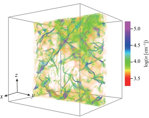
Volume rendering map of density at t = 0.6 Myr (reproduced from Inoue & Fukui 2013). (Color online)
Model parameters.
| Parameter | Value |
|---|---|
| 〈n〉0 | 300 cm−3 |
| Δn/〈n〉0 | 0.33 |
| B0 | 20 μG |
| Vcoll | 10 km s−1 |
| Resolution | (8.0/512) pc |
| Parameter | Value |
|---|---|
| 〈n〉0 | 300 cm−3 |
| Δn/〈n〉0 | 0.33 |
| B0 | 20 μG |
| Vcoll | 10 km s−1 |
| Resolution | (8.0/512) pc |
Model parameters.
| Parameter | Value |
|---|---|
| 〈n〉0 | 300 cm−3 |
| Δn/〈n〉0 | 0.33 |
| B0 | 20 μG |
| Vcoll | 10 km s−1 |
| Resolution | (8.0/512) pc |
| Parameter | Value |
|---|---|
| 〈n〉0 | 300 cm−3 |
| Δn/〈n〉0 | 0.33 |
| B0 | 20 μG |
| Vcoll | 10 km s−1 |
| Resolution | (8.0/512) pc |
3 Structure of the shock-compressed layer and the formation of the dense cores
3.1 The shock-compressed layer
The colliding gas has inhomogeneous density distribution. The flows create the compressed layer between them, which becomes decelerated and denser. Figure 2a shows the velocity vectors in an x–y plane on the negative x-side, and the behavior is similar on the positive x-side. Figure 2b shows a close up in the velocity transition zone at an epoch of 0.7 Myr. The velocity does not change from the initial value at x less than −1.0 pc, and quickly becomes small and completely randomized in angle as x ranges from −1.0 to −0.6 pc. This change is due to the shock dissipation and momentum exchange between the colliding flows. Figures 2c–2f show the averaged velocity, the angle between the velocity vector and the x-axis, the gas density, and pressure, respectively, as a function of x, and show that the velocity decreases to ∼2 km s−1 from 12 km s−1 and is randomized in direction. In figures 2a and 2b, velocity is larger than the initial value 10 km s−1 because of the gravitational acceleration by the shock-compressed layer.
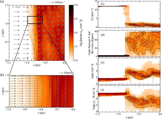
(a) Projected velocity vectors (arrows) overlaid on distribution of mean density (image) in |z| < 0.08 pc at t = 0.7 Myr. (b) Close-up view of (a). (c) Distribution of size of velocity vector (|$|{\boldsymbol V}|$|), (d) angle between velocity vector and the x-axis, (e) density n and (f) dynamic pressure for each pixel. The contours in panels (c)–(f) contain |$30\%$|, |$60\%$|, and |$90\%$| of data points but excluding gas with initial condition (|$|{\boldsymbol V}|\gtrsim 12\:$|km s−1 and angle ∼0°). (Color online)
The time-evolution of the layer is shown as a density distribution along the x-axis at each epoch in figure 3. In 0.3 Myr the maximum density becomes more than 105 cm−3 and the fraction of the dense gas increases in time. Table 2 shows the gas mass in the compressed layer above 104 cm−3. The full thickness of the compressed dense layer above 104 cm−3 is ∼1.5 pc in the x-direction. After 0.4 Myr we find sharp narrow spikes which indicate the formation of filaments and dense cores in the layer, as detailed later. The fraction of the dense gas above 105 cm−3 is |$10\%$|–|$17\%$| of the total gas mass of density above 104 cm−3. Figure 4 shows a probability distribution function of density, where t = 0.0 Myr shows the initial condition. The collision creates the higher density tail above 104 cm−3 as well as the low-density tail below the initial density distribution produced by turbulence. The high-density tail characterizes the compression as expressed by a power law with an index range from −3.0 to −2.0, which becomes flatter in time.
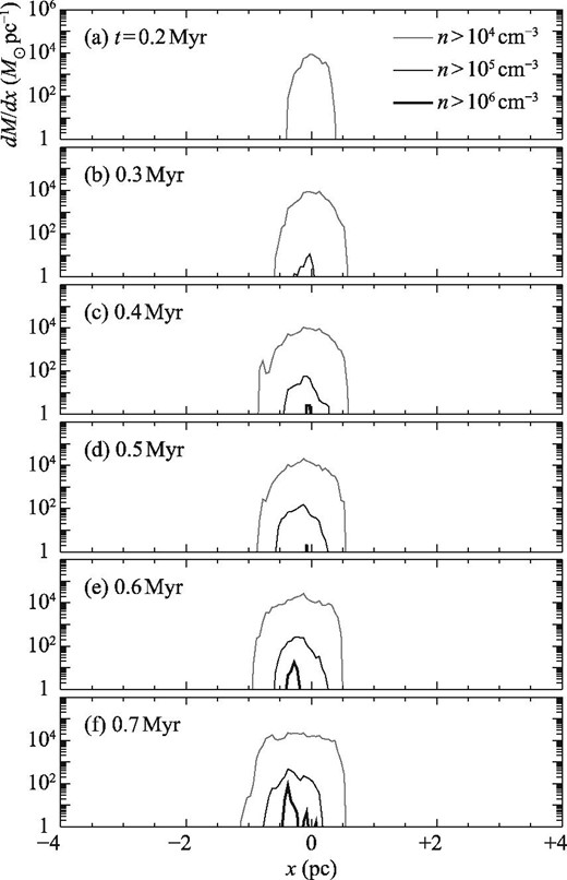
(a) Distribution of dense molecular gas along the x-axis at t = 0.2 Myr. (b)–(f) Same as panel (a) but for t = 0.3–0.7 Myr. Gray, thin black, and thick black lines in each panel show n > 104 cm−3, n > 105 cm−3 and n > 106 cm−3, respectively.
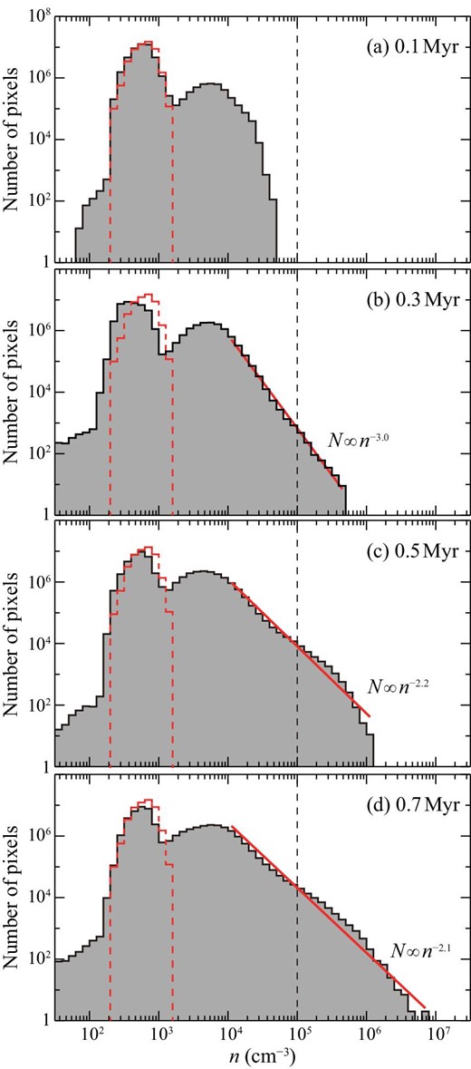
(a) Histogram of H2 density for each pixel in a range of −1.5 pc < x < +1.5 pc at t = 0.1 Myr. The histogram at t = 0 is also shown by the red dashed line. (b)–(e) Same as panel (a) but for t = 0.1, 0.3, 0.5 and 0.7 Myr. The vertical dashed line in each panel shows n = 105 cm−3. (Color online)
Mass of dense gas.
| Mass (|$M_{\odot }$|) | |||
|---|---|---|---|
| t (Myr) | n > 104 cm−3 | n > 105 cm−3 | n > 106 cm−3 |
| 0.2 | 2800 | — | — |
| 0.3 | 4100 | 31 | — |
| 0.4 | 5700 | 310 | 5 |
| 0.5 | 9400 | 970 | 3 |
| 0.6 | 13000 | 1800 | 38 |
| 0.7 | 18000 | 2900 | 140 |
| Mass (|$M_{\odot }$|) | |||
|---|---|---|---|
| t (Myr) | n > 104 cm−3 | n > 105 cm−3 | n > 106 cm−3 |
| 0.2 | 2800 | — | — |
| 0.3 | 4100 | 31 | — |
| 0.4 | 5700 | 310 | 5 |
| 0.5 | 9400 | 970 | 3 |
| 0.6 | 13000 | 1800 | 38 |
| 0.7 | 18000 | 2900 | 140 |
3.2 Dense cores in the filaments
The density distribution in the three-dimensional space is characterized by filaments which include dense cores. Figure 5a shows the distribution of filamentary distribution identified as connected regions with n > 105 cm−3, where different filaments are indicated by different arbitrary colors. In each filament we define dense cores by using the CLUMPFIND algorithm (Williams et al. 1994). The algorithm is designed to be applied to spectral line datasets, T(x, y, V) data cubes, but here we use it to find cores in n(x, y, z) datasets.
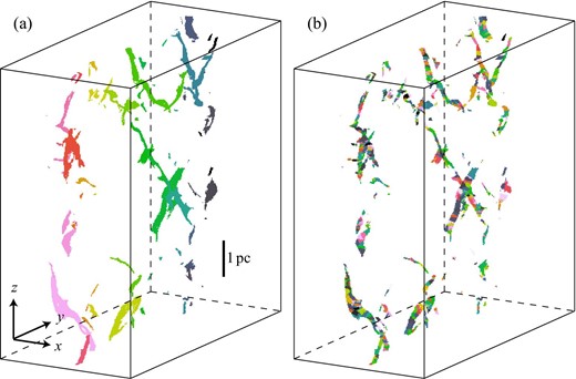
The distribution of (a) filamentary distribution, identified as connected region with n > 105 cm−3, and (b) dense cores defined by using CLUMPFIND algorithm (Williams et al. 1994). Different filaments/cores in panels (a) and (b) are indicated by different arbitrary colors. (Color online)
Inoue and Fukui (2013) explained that the distorted field lines guide the gas flow into dense cores in a filamentary shape (see their figure 1). The created filaments are generally oriented in the perpendicular direction to the magnetic field. Filament formation is a common feature in a collision-compressed layer as shown in the other simulations of cloud–cloud collision (Inoue et al. 2018). In this particular simulation by Inoue and Fukui (2013), because the two colliding gas flows have different magnetic field orientations (perpendicular to each other), the directions of the resulting filaments are often crossing at 90°. This crossing feature disappears if the magnetic field orientations are similar between the colliding clouds. Note that the crossing feature does not affect the mass distribution of the dense cores. We look into more details in figure 6, where the magnetic field lines and the velocity vector are projected in two typical regions with filaments. In figures 6a-1 and 6b-1 we find a common feature that the filaments are well-aligned in a direction perpendicular to the field line. The velocity vectors in figures 6a-2 and 6b-2, on the other hand, do not show a systematic trend and are not always aligned with the field lines. This suggests that the gas motion has both parallel and perpendicular components near the filaments, whereas the time-average produces the net gas flow into the filaments. We also notice that the line mass in a filament, which ranges from 20 to |$150\, M_{\odot }\:$|pc−1, tends to increase if the velocity vectors and field lines are in a similar direction, as suggested in figure 6b.
![Projected magnetic field vector (a)-1 and velocity vector (a)-2 shown in a typical region with filaments. The magnetic field vector and velocity vector are given as ${\boldsymbol B}=\sum _\mathrm{filament}\left[{\boldsymbol B}(x)n(x)\Delta x\right]/\sum _\mathrm{filament}\left[n(x)\Delta x\right]$ and ${\boldsymbol V}=\sum _\mathrm{filament}\left[{\boldsymbol V}(x)n(x)\Delta x\right]/\sum _\mathrm{filament}\left[n(x)\Delta x\right]$, respectively, where the summation is along the x-axis (perpendicular to the page). (b)-1, (b)-2 Same as panels (a)-1 and (a)-2 but for another sample. (Color online)](https://oup.silverchair-cdn.com/oup/backfile/Content_public/Journal/pasj/73/Supplement_1/10.1093_pasj_psaa079/3/m_psaa079fig6.jpeg?Expires=1749210766&Signature=yl2OSo6YKUbk0FYURQmLptuJouUeD0lk~rR3ZUTLr7A~9ZHWGQz5Tcp02Q3HAghpQuaGfumrbU4DGtSaNc7XLbEMQ7TQ5YytX9MunPcsx5arW0x3~sO~dSRtHbWoPs84szdNBsRDkORzwH4zmtDCrnn4bKv9t4JI0YqaA4AWZaV9-R9kz05t~ZfSuuAX~nHBEz6HzcC25joaZ2iyNw9HfUxwB6iPlKCQdMkY2Y7qzo0bE2SszUTr7p47hpVZIwvqTCM0e6zFxGD7XrOeu4HpT8faMUjMRbsptqApXUlkxn9yCnvZdjeDuNIP6MgJTntBemNPntg7M~287YDO3GFXEQ__&Key-Pair-Id=APKAIE5G5CRDK6RD3PGA)
Projected magnetic field vector (a)-1 and velocity vector (a)-2 shown in a typical region with filaments. The magnetic field vector and velocity vector are given as |${\boldsymbol B}=\sum _\mathrm{filament}\left[{\boldsymbol B}(x)n(x)\Delta x\right]/\sum _\mathrm{filament}\left[n(x)\Delta x\right]$| and |${\boldsymbol V}=\sum _\mathrm{filament}\left[{\boldsymbol V}(x)n(x)\Delta x\right]/\sum _\mathrm{filament}\left[n(x)\Delta x\right]$|, respectively, where the summation is along the x-axis (perpendicular to the page). (b)-1, (b)-2 Same as panels (a)-1 and (a)-2 but for another sample. (Color online)
Each filament contains dense cores. Formation of similar dense cores is observed in the non-MHD numerical simulations of a cloud–cloud collision by Takahira, Tasker, and Habe (2014), which is due to cloud self-gravity. In order to characterize the cores we applied the clump-find algorithm to the filaments at nthreshold, and identified 777 cores in total at 0.7 Myr, as shown in figure 5b. In each epoch the physical parameters, including mass, size, and average density of the dense cores, are derived for density above 105 cm−3. The mass of a core is the sum of all of the pixels, and the size of a core is calculated as the geometrical mean of three major axes, which are derived by fitting a spheroid with three semi-major axes a, b, and c. Figure 7a shows a scatter plot between mass and size of the dense cores, figure 7b a size histogram, and figure 7c a scatter plot between the axial ratios, a/b and b/c. The mass of the core is in the range 0.1–|$100\, M_{\odot }$| with size in the range of 0.01–0.1 pc. The maximum mass of the core attained is close to |$100\, M_{\odot }$| with a size of 0.1 pc at density above 105 cm−3, while it depends on the threshold density adopted. The aspect ratios a/b and b/c are mostly in the range of 1–3 with an average of 1.9–2.5, indicating that they are not spherical: |$15\%$| of the cores are spherical, |$35\%$| prolate, and |$50\%$| oblate. For the prolate and oblate cores we made histograms of an angle between the major axis and the field lines in figure 8a and the minor axes and the field lines in figure 8b. We find that the prolate cores are aligned within 40° to the field lines, while the oblate cores have minor axes with an angle to the field lines in a broad range of 10°–70°. The former seems to be a natural result of the prolate core formation in a filament, while the oblate cores form more randomly.
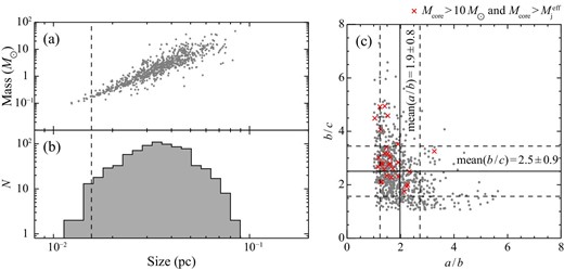
(a) Mass–size diagram and (b) size histogram for the identified cores at t = 0.7 Myr. The sizes are derived as geometric mean of the major-axis length a, second-major-axis length b and minor-axis length c. The vertical dashed lines in panels (a) and (b) show the pixel size (1.6 × 10⁻² pc). (c) Scatter plot between b/c vs. a/b. The red crosses are the cores with |$M_\mathrm{core}>10\, M_{\odot }$| and |$M_\mathrm{core}>M_\mathrm{j}^\mathrm{eff}$|. The vertical solid- and dashed-lines show mean and standard deviation of a/b and the horizontal ones show those of b/c. (Color online)
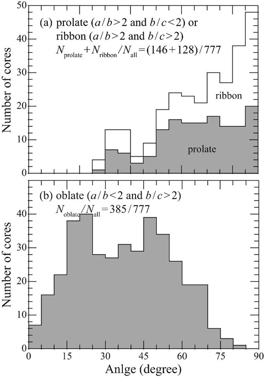
(a) Histogram of angle between magnetic field vector and major-axis for prolate (a/b > 2 and b/c < 2, gray shaded) and ribbon-like morphology cores (a/b > 2 and b/c > 2). (b) Histogram of angle between magnetic field vector and minor-axis for oblate cores with a/b < 2 and b/c > 2.
3.3 A core mass function
Figure 9 shows a core mass function, and the ratio of the core mass Mcore to the effective Jeans mass |$M_\mathrm{j}^\mathrm{eff}$|, which counts the turbulent and magnetic pressure in addition to the thermal pressure, and to the Jeans mass Mj, which counts only the thermal pressure, as a function of the core mass at five epochs. The cores grow by the collisional compression. We find an increase of the cores in the mass range 0.1–|$10\, M_{\odot }$| and the highest mass above 105 cm−3 reaches ∼50 |$M_{\odot }$| at 0.7 Myr. We see a clear signature of a top-heavy mass function extending beyond |$10\, M_{\odot }$| in figure 9. The ratio between the core mass and the effective Jeans mass shows that most of the cores with mass more than |$10\, M_{\odot }$| are gravitationally bound and will become high-mass protostars, as shown by Inoue and Fukui (2013) and Inoue et al. (2018). Dense cores with masses less than |$10\, M_{\odot }$| are more weakly gravitationally bound. They may form low-mass stars if the core mass is greater than the Jeans mass, depending on the details of the gas dynamics. In this sense, the number density of the cores whose mass lies between |$0.3\, M_{\odot }$| and |$10\, M_{\odot }$| in figure 9 gives an upper limit for the number density of the low-mass protostars. It is unlikely that cores that are less massive than the Jeans mass form stars, while the less-massive cores may grow into more massive ones by mass accretion and coagulation, depending on the time scale before dissipation by ionization due to the forming O stars.
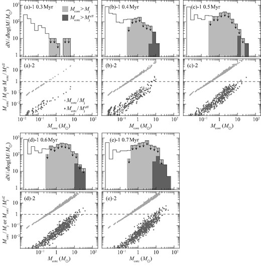
Upper panels: Core mass function (CMF) for (a) t = 0.3 Myr, (b) 0.4 Myr, (c) 0.5 Myr, (d) 0.6 Myr, and (e) 0.7 Myr. Light- and dark-gray show CMF for Mcore > Mj and |$M_\mathrm{core}>M_\mathrm{j}^\mathrm{eff}$|, respectively. Lower panel: Mcore/Mj and |$M_\mathrm{core}/M_\mathrm{j}^\mathrm{eff}$| ratios plotted against Mcore. The horizontal dashed lines show Mcore = Mj (|$M_\mathrm{core}=M_\mathrm{j}^\mathrm{eff}$|).
The present model prediction of the core mass function consists of the high-mass part for 6–|$50\, M_{\odot }$| (dark gray in figure 9e-1) and the low-mass part for less than |$20\, M_{\odot }$| (light gray in figure 9e-1). For the cores in the low-mass part, it remains to be tested numerically if they really become gravitationally unstable to form stars. The high-mass part indicates the mass function of the gravitationally unstable cores and is robust. The low-mass part gives upper limits for the number of the cores leading to star formation. If the cores can fragment further, the low-mass part may be affected. Given that the most unstable scale-length L of gravitational instability for a filament of width W is L = 4W (Inutsuka & Miyama 1992), the cores identified in our simulation that have a typical aspect ratio of 1.9–2.5 are the structures that are fragmented from a longer filament. Further heavy fragmentation, therefore, does not seem to occur. Recent simulations that followed the gravitational collapse phase of a filamentary core created by a cloud collision show that the massive filamentary core collapses into a massive sink (Inoue et al. 2018). Note that we never claim that each massive core found in our analysis certainly evolves into one massive star with high star formation efficiency. The cores can fragment during the collapse phase. However, recent theoretical studies suggest that once the massive compact core is created, its collapse will eventually create massive star(s), i.e., the collapse of a massive core would not result in the formation of many low-mass stars due to heavy fragmentations (Krumholz et al. 2009; Rosen et al. 2016) In addition, the massive star formation time-scale is very short in the order of 5 × 10⁴ yr once the core is formed (Krumholz et al. 2009), in the order of the free-fall time 105 yr for 105 cm−3. It is therefore likely that the star(s) begin to warm up the surrounding gas rapidly, and further fragmentation of the rest of the cores is not very effective (Krumholz 2006). All these features allow us to compare our core analysis with observations at least in high-mass star forming regions.
4 Properties of the dense cores and O stars
The present results on dense cores provide an insight into the O star formation by cloud–cloud collision. We first describe the formation of individual O stars in dense cores, and secondly present the predicted mass function and spatial distribution of multiple O stars.
4.1 O star formation and subsequent evolution in the shock-compressed layer
In the shock-compressed layer, dense cores smaller than 0.1 pc with maximum mass close to |$100\, M_{\odot }$| are created. These cores have density greater than 105 cm−3 and become gravitationally unstable. Inoue and Fukui (2013) showed that the mass-accretion rate in the shock-compressed layer is greater than ∼10−4 |$M_{\odot }\:$|yr−1 due to the enhanced effective sound speed, which is large enough to overcome the radiation pressure to form high-mass stars (Wolfire & Cassinelli 1987). The formation time-scale of a |$15\, M_{\odot }$| O star is estimated to be |$15\, M_{\odot } /10^{-4}\, M_{\odot }\:\mbox{yr}^{-1} = 0.15\:\mbox{Myr}$| if a constant mass accretion rate is assumed. In this mass-accretion phase, we expect molecular outflow is generated as driven by the accretion disk in a dynamical time scale of ∼104 yr (e.g., Machida et al. 2008). When the star becomes as massive as |$15\, M_{\odot }$|, its surface temperature reaches 30000 K (Cox 2000), which is high enough to emit significant ionizing photons to its surroundings. The ionization then proceeds at a typical speed of more than a few km s−1 (e.g., Hosokawa & Inutsuka 2005), and in a few times 0.1 Myr a radius of ∼1 pc will be ionized, while a significant portion of the neutral gas generally remains unionized outside the radius.
The O star formation is a natural outcome of cloud–cloud collision, a rapid process which converts the low-density molecular gas to dense gas in 0.1 Myr. It is essential that the compression is done not by self-gravity but by the magnetic-field guided supersonic flow. This rapidity is the key to collect large mass of |$100\, M_{\odot }$| into a 0.1-pc volume. If the collection process is slow, in the order of the free-fall time (∼ Myr for density 1000 cm−3), it is likely that the gas is consumed by the formation of low-mass stars before being collected in the volume.
Gravitational contraction of a dense core is numerically simulated by Krumholz et al. (2009) at highest resolution of 100 au, and they used |$100\, M_{\odot }$| within a radius of 0.1 pc with a power-law distribution at the initial condition. The results show that two stars with mass of |$40\, M_{\odot }$| and |$30\, M_{\odot }$| form, with a remaining |$30\, M_{\odot }$| of gas, where star formation efficiency (SFE) is |$70\%$|. The two stars are formed rapidly, on a time scale of 5 × 10⁴ yr. Their core is similar to the typical massive unstable cores formed under cloud–cloud collision of the present work. These authors adopted the typical massive core observed in high-mass star forming regions, and did not explore the core formation mechanism.
4.2 Cluster formation in the collision-compressed layer
4.2.1 Formation of filaments and O stars in the compressed layer
A cloud–cloud collision produces the filamentary morphology of the compressed layer and the dense-core distribution confined to the filaments as shown in figure 10. The O stars formed will not move by more than 0.2 pc within 0.1 Myr, the typical time scale of the O star formation, for an average velocity of dense cores of ∼1 km s−1 (figure 2). This indicates that the O star distribution is determined by the collision-formed filamentary distribution until gravitational relaxation becomes effective later, in more than Myr. The evolution of the stellar system in this phase is essentially similar to that given by N-body simulations (e.g., Fujii & Portegies Zwart 2015). The filaments will be destroyed in the order of 0.1 Myr by the ionization once the stars become as massive as 15 |$M_{\odot }$|, and the final mass of the formed stars, i.e., the O stars and their neighbors, are determined by the mass of the dense cores and the duration of the mass accretion until full ionization. In the following we assume for simplicity that the mass of the gravitationally unstable dense cores is converted into the stellar mass, while the conversion efficiency may be somewhat less than 1.0. The numerical simulation result for instance shows that SFE is 0.7 for a |$100\, M_{\odot }$| core within 0.1 pc (Krumholz et al. 2009). In the present simulations no ionization is incorporated. In figure 10 we draw a circle of the ionization front for each “O star” by assuming for simplicity that the ionization front proceeds at a uniform speed of 3 km s−1 after a dense core of |$10\, M_{\odot }$| with density 105 cm−3 appears. This allows us to have a rough idea of the dispersal of the filaments by ionization.

Column density map of H2 (low-density gas with <104 cm−3 is excluded) in the y–z plane at (a) t = 0.4 Myr, (b) 0.5 Myr, (c) 0.6 Myr, and (d) 0.7 Myr. The crosses show the positions of massive cores with |$M_\mathrm{core}>10\, M_{\odot }$| and |$M_\mathrm{core}>10\, M_\mathrm{j}^\mathrm{eff}$|, and the dots show intermediate mass cores with |$M_\mathrm{core}=5\!-\!10\, M_{\odot }$|. Circles show ionization front in “H ii regions” which proceeds at a uniform speed of X km s−1 after dense cores with |$M_\mathrm{core}>10\, M_{\odot }$| and |$M_\mathrm{core}>10\, M_\mathrm{j}^\mathrm{eff}$| appear. (Color online)
We obtain a further insight into the O star formation by inspecting column density in the filaments. Figure 11 shows the column density distribution in space for eight regions of 1.5 pc × 1.5 pc in the y–z plane, selected by the number of O stars and the distribution function of column density in each box. Figure 11 indicates that O stars can be formed in isolation and/or in a cluster depending on the resultant column density. In the distribution function of column density in figure 8, the typical column density peaks are found at around 1022 cm−2. Formation of nearly 10 O stars occurs in a filament with high column density tails beyond 1023 cm−2 [Regions (2), (3), (4), and (6)]. On the other hand, in a region of a single or no O star formation, the column density distribution is not extended beyond 1023 cm−2.
![Column-density map of H2 (low-density gas with <104 cm−3 is excluded) in the y–z plane at t = 0.7 Myr (top left-hand panel) and column density histogram in the eight regions of 1.5 pc × 1.5 pc [panels (1)–(8)]. The crosses in the top left-hand panel show the positions of massive cores with $M_\mathrm{core}>10\, M_{\odot }$ and $M_\mathrm{core}>10\, M_\mathrm{j}^\mathrm{eff}$, and the dots show intermediate-mass cores with $M_\mathrm{core}=5\!-\!10\, M_{\odot }$. (Color online)](https://oup.silverchair-cdn.com/oup/backfile/Content_public/Journal/pasj/73/Supplement_1/10.1093_pasj_psaa079/3/m_psaa079fig11.jpeg?Expires=1749210766&Signature=nd1AWtINZ5FNx8d79gWFoycuXqp7Ks40pjdgXChTdaa285vuZ~Vaz~PwdVG72oPcJg6LwrTrgdZwOSzevnWXqr7jfBHAhxZCaqUwx33WwLJN7Qcl39pDre3EYGvK2sKmTKkluvHiBBSA3quqmF3IGyLz8kuwOW2siQCNjeKH9HzdngwTt5Rl3fGTLx1Nmeljtrr4OC-d5i8w9z9hsQndFmObb1SKC17itO2wPhn5u5ap3cD4ET~kH4POceR2Z~tVIYrSrIRT7i0E2qJFBRy0oSD9xj2E~FFK6SIZ6O-tCrqiFfiT82JMx0NfEdQqcPjfZsc1mBSzFKhqmufBpH~VbA__&Key-Pair-Id=APKAIE5G5CRDK6RD3PGA)
Column-density map of H2 (low-density gas with <104 cm−3 is excluded) in the y–z plane at t = 0.7 Myr (top left-hand panel) and column density histogram in the eight regions of 1.5 pc × 1.5 pc [panels (1)–(8)]. The crosses in the top left-hand panel show the positions of massive cores with |$M_\mathrm{core}>10\, M_{\odot }$| and |$M_\mathrm{core}>10\, M_\mathrm{j}^\mathrm{eff}$|, and the dots show intermediate-mass cores with |$M_\mathrm{core}=5\!-\!10\, M_{\odot }$|. (Color online)
4.2.2 Cluster formation scenario
A cloud–cloud collision creates massive dense cores, precursors of an O star, which are clustered in a filament. In order to illuminate the whole process of a cluster formation, we present a formation scenario of an O-star cluster as a two-step process, i.e., (i) pre-collision phase and (ii) post-collision phase, in the following. Similar discussion is given for two individual objects RCW 38 and the Orion Nebula Cluster (ONC), from an observational point of view (Fukui et al. 2016, 2018a).
In the pre-collision phase, the two clouds independently form only low-mass stars from low-mass cores without mutual interaction if they are dense enough: a typical observed case is the Taurus cloud complex forming ∼20 low-mass stars in a cloud of mass |$\sim 1000\, M_{\odot }$|, size ∼5 pc and column density (1–10) × 1021 cm−2 (Mizuno et al. 1995; Onishi et al. 1996, 1998, 2002). The time scale of this phase can be as long as several Myr, forming low-mass stars at a mass accretion rate of 10−6 |$M_{\odot }\:$|yr−1 in the non-shocked condition as long as the cloud dispersal by outflows/winds is not substantial. The core mass function is shown in Onishi et al. (2002), which indicates that the dense core of density 105 cm−3 has a mass range of from 1 to |$10\, M_{\odot }$|, which can be roughly converted to a stellar mass range of from 0.1 to |$1\, M_{\odot }$|.
Suppose an accidental collision between two such clouds happens at a supersonic velocity in the order of 10 km s−1; the collision rapidly creates the collision-compressed layer in ∼0.1 Myr to form massive dense cores (the post-collision phase). The moment of the collision is subject to a stochastic process among the clouds in the Galactic disk with a typical mean free time of less than 10 Myr depending on the cloud number density, as shown by numerical simulations (e.g., Kobayashi et al. 2018; see also Fujimoto et al. 2014; Dobbs et al. 2014). The number of O star(s) depends on the cloud column density. Based on the previous observations of cloud–cloud collisions, Fukui et al. (2018a) showed that a single O star can be formed for total column density of 1022 cm−2, and that formation of nearly 10 O stars requires a total column density as high as 1023 cm−2 at a 1 pc scale (see also Enokiya et al. 2021). Clouds with column density below 1022 cm−2 will grow in mass by collision without O star formation.
Subsequently, the massive dense cores form O stars which ionize the clouds and suppress subsequent star formation, the details of which depend on the number of the O stars, and the density and size of the clouds. At the end of this phase, a cluster becomes exposed by ionization, and the emerging cluster consists of old low-mass stars extended over the clouds and young O star(s) localized within the colliding area. Consequently, the age of the low-mass members can be distributed from 1 Myr to several Myr as determined by the collision mean free time, and the age of the O stars is peaked just after the collision with a short duration in the order of 0.1 Myr. Such a short time-duration is supported by the detailed observations of stellar ages in two clusters, NGC 3603 and Westerlund 1 (Kudryavtseva et al. 2012). In ∼1 Myr after the O star formation the ambient gas will be fully ionized and dispersed, as seen in NGC 3603 and Westerlund 1. After the ionization, gravitational relaxation will redistribute the filamentary O stars into a more centrally concentrated stellar cluster in a few Myr, as is modeled by the N-body numerical simulations (e.g., Fujii & Portegies Zwart 2015).
For example, the ONC and RCW 38 correspond to the earliest post-collision phase of 0.1 Myr after collision, and NGC 3603 is of 2 Myr after the ionization. The pre-collision phase is not easily recognized observationally at a usual distance of O stars more than 1 kpc because a pre-collision cluster without O stars is not obvious in the Galactic plane due to extinction and contamination.
5 Comparison with observations of O stars triggered by a cloud–cloud collision
Recent studies show that cloud–cloud collision is an essential process in high-mass star formation. Observationally, cloud–cloud collision is found in many high-mass stars associated with molecular clouds which are not fully ionized. Here we compare the present theoretical results with observations of cloud–cloud collisions in the youngest phase of ∼0.1 Myr, where we are able to find the O star distribution just after their formation without ionization or gravitational relaxation. The key features of the O star formation derived in the present work and Inoue and Fukui (2013) are summarized as follows:
(a) Cloud–cloud collision is a mechanism of rapid formation of massive dense cores with density of 105 cm−3 up to |$\sim 50\, M_{\odot }$| in 0.7 Myr, which is characterized by a top-heavy mass function. The massive dense cores are gravitationally unstable and lead to O star formation under the high-mass accretion rate. Cloud–cloud collision is therefore a mechanism of O star formation. Less-massive dense cores, some of which may be transient, are also formed in greater number than the massive dense cores in the collision compressed layer, while a small fraction of them perhaps becomes gravitationally unstable to form low-mass stars.
(b) The colliding gas flow of 10 km s−1 is quickly decelerated to around 1.5 km s−1 in the collisional-shocked layer, where the velocity vector becomes randomized. The collision-compressed layer of ∼1 pc thickness becomes filamentary with 0.1 pc width, where the gas flow is guided to a filament by the magnetic field lines. The formation of the filament is not due to the self-gravity and is, therefore, more rapid in ∼0.1 Myr than the free-fall time, ∼1 Myr for 1000 cm−3, which is essential in O star formation. Once a filament is formed, the filament grows in mass by the incoming flow. In the filament the massive dense cores are formed by self-gravity in a 0.1 pc scale in free-fall time of 0.1 Myr for density above 105 cm−3.
(c) The massive dense cores form O stars which are confined in the filament, and the O star distribution is filamentary, having the same velocity field as the collisional shocked layer. When a mature O star of more than |$15\, M_{\odot }$| forms, the ionization by the O star becomes effective in dispersing the gas and quenches star formation within a few pc of the O star(s). The ionization removes gas and the O star distribution evolves by gravitational relaxation in a Myr time scale.
For a comparison with the observations we use the two properties of the dense cores of the present work; the separation between the cores and the core mass function.
Figure 12a shows a histogram of the separation between dense cores with mass greater than |$5\, M_{\odot }$| in the y–z plane. The separation is peaked at 0.1 pc and is extended up to a few pc. The cores more massive than |$10\, M_{\odot }$| show two peaks at ∼0.1 pc and ∼1 pc, where the small value reflects the core distribution within a filament and the large one the core distribution between filaments. The distribution provides a test tool for a comparison with observations. Figure 13 shows another comparison of the core mass function in the collision compressed layer taken from figure 9. The core mass function in cloud–cloud collision is top-heavy with a negligible contribution of dense cores less than |$1\, M_{\odot }$|. The initial mass function (IMF) of field stars is shifted to lower mass by more than an order of magnitude as compared with that in cloud–cloud collision (e.g., Kroupa 2001; Chabrier 2005), whereas a direct comparison between cores and stars requires exact SFE and multiplicity of stars. The separation between the cores are compared both with the observed cores and stars in the following by assuming that they do not move over a distance of more than 0.1 pc in 0.1 Myr. The cores in the core mass function include those which are not gravitationally unstable. Therefore, the core mass function is not the stellar mass function, and a core may form two or more stars with SFE lower than 1.0. Such a comparison is valid as long as it is made only for the cores and not for the stars.
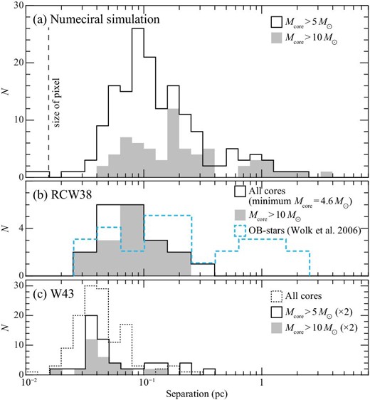
(a) Histogram of core-to-core separation for |$M_\mathrm{core}>5\, M_{\odot }$| at t = 0.7 Myr and those for |$M_\mathrm{core}>10\, M_{\odot }$| (gray shaded). Here, the separations are given as edge-lengths of two-dimensional (projected along the x-axis) minimum-spanning-trees (MSTs) of cores. (b) Same as panel (a) but for RCW 38 dense condensations (Torii et al. 2021) and OB-star candidates (Wolk et al. 2006). (c) Same as panel (a) but for W 43 cores (Motte et al. 2018). (Color online)
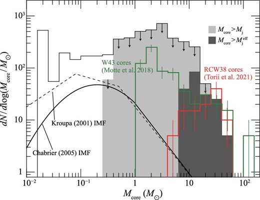
CMF at t = 0.7 Myr (identical to figure 9e-1). Those for RCW 38 cores (Torii et al. 2021) and W 43 cores (Motte et al. 2018) are superimposed. The error bars correspond to |$\sqrt{N}$| statistical uncertainties. The dashed line shows the single-star IMF of Kroupa (2001) and the solid curve shows the system IMF by Chabrier (2005). (Color online)
Super star clusters in the Milky Way include 10–20 O stars in a parsec-scale in addition to ∼104 low-mass stars that are more extended (see for a review Portegies Zwart et al. 2010; Ascenso 2018). Among them, the very rich clusters, including O stars as young as 0.1 Myr, are the primary sites to test the collision signatures, separations between dense cores (or O stars), and a core mass function, which will be rapidly lost by ionization in Myr.
5.1 RCW 38
As the best cluster for comparison we focus on RCW 38, the youngest super star cluster, where O star formation was triggered by a cloud–cloud collision according to Fukui et al. (2016). Most recently, Torii et al. (2021) mapped the CO clouds with ALMA at high resolution of ∼2″ in C18O J = 2–1 emission and resolved 21 dense cores larger than 0.01 pc with a mass detection limit of |$\sim 6\, M_{\odot }$|. The O star candidates (Wolk et al. 2006; Winston et al. 2011) are distributed in filamentary distribution of ∼1 pc length toward the collisional area of radius 0.5 pc, as shown in figure 1 of Torii et al. (2021). Figure 12d shows that separations between the dense cores/O stars are consistent with the present results. In figure 13 the core mass function is compared, showing also good correspondence in a virial mass range of 8–|$50\, M_{\odot }$|. The C18O cores in RCW 38 are often gravitationally unstable, as shown by the virial mass which is calculated to be smaller than the molecular mass (see their table 3). They are probable “protostellar” cores, which is also supported by two of the RCW 38 cores with protostellar outflow. Higher-sensitivity observations in RCW 38 will reveal lower-mass cores which cover a wider mass range. The top-heavy core mass function in RCW 38 is consistent with the collisional compression, and also the separations of the massive dense cores and the O stars. The dense gas which is included in the detected dense cores is |$360\, M_{\odot }$|, which corresponds to |$33\%$| of the total mass of the dense gas detected in the C18O (J = 2–1) emission (Torii et al. 2021), although cores with mass below |$6\, M_{\odot }$| are not spatially resolved. This fraction may be compared with the total mass of the unstable massive cores in the present simulations, |$650\, M_{\odot }$|, which corresponds to |$22\%$| of the total mass of the gas with density above 105 cm−3. Both show a significantly high fraction of the massive cores.
We test the physical parameters of the clouds into more detail. The total number of the massive dense cores and O star candidates in RCW 38 is ∼40 for an area of ∼0.5 pc × 0.5 pc and the projected density of cores/O stars is ∼160 pc−2, 10 times higher than in Region (6) of the present results. The age of RCW 38 is in the order of 0.1 Myr, which is significantly shorter than the 0.7 Myr of the present model. These suggest that the initial density of the parent cloud of RCW 38 may be significantly higher than the present initial density of 300 cm−3. Inoue and Fukui (2013) showed a case with an initial density of 1000 cm−3, three times higher than the present model [model No. 4 in Inoue and Fukui (2013)], which indicates more rapid dense core formation and higher column density in the compressed layer. A rough estimate indicates that an initial density of more than 104 cm−3 may be appropriate to explain these differences, which needs to be confirmed by further MHD simulations. It is desirable to have more objects to be tested, whereas most of the other massive clusters in the Milky Way studied in detail so far are not so young as RCW 38. The only possible exception is the ONC, which is worth testing by a uniform survey for dense cores with ALMA over the collisional area. The collisional age of the O stars in the ONC is 0.1 Myr (Fukui et al. 2018a), and such observations will shed new light on this issue.
5.2 W 43
W 43 is a remarkable mini-starburst in the Milky Way which attracted keen interest in understanding high-mass star formation. Recently, Kohno et al. (2021) made a detailed analysis of the molecular clouds in W 43 and found evidence for multiple cloud–cloud collisions in triggering high-mass star formation. In one of the proto clusters in W 43 Main, new ALMA observations were used to resolve dense cores with unprecedented details by Motte et al. (2018). These authors obtained a core mass function of 130 dense cores with density ∼107–1010 cm−3 covering a mass range 1–|$100\, M_{\odot }$| in dust continuum emission with a mass detection limit of |$1.6\, M_{\odot }$|, while linewidths and other kinematic information are not available. The cores may be protostellar, if we consider the active high-mass star formation in W 43 Main (Motte et al. 2018; Kohno et al. 2021), while their gravitationally stability is not shown by spectroscopic data. Figure 1 of Motte et al. (2018) shows the dust image where we find highly filamentary dust distribution with dense cores. The filaments have ∼0.1 pc width and ∼0.5 pc length and the mass of the dense cores are derived. The formation of filaments by a cloud–cloud collision is a plausible mechanism applicable to W 43. The separations between the dense cores as shown in figure 12 e have a peak at ∼0.4 pc, which is similar to but somewhat smaller than in RCW 38. The core mass function is plotted from Motte et al. (2018) in figure 13 and shows that the core mass function is consistent with the present one, in particular at the high-mass end of the present function in the range 8–|$50\, M_{\odot }$|. The massive dust cores having more than |$6\, M_{\odot }$| occupy |$70\%$| of the total mass of the detected dust cores, |$880\, M_{\odot }$|. This may indicate a more top-heavy mass function than in RCW 38, and the higher density environment of W 43 may be responsible for it.
6 Dependence on the model parameters
The present results depend on the parameters adopted in the simulations by Inoue and Fukui (2013). The model is idealized as compared with the real cloud–cloud collision, whereas no fine-tuning of the parameters is made. We discuss possible adjustments of the parameters for a more sophisticated model.
The size of the present collision area, 8 pc × 8 pc, is larger than the typical area of 1 pc2 in the cloud–cloud collisions in the Milky Way. This difference perhaps causes higher gas peak column density in the present results than a smaller area by collecting mass in directions perpendicular to the collision. The size of the model cloud length, which is assumed to be as long as 7 pc by setting the final epoch to be 0.7 Myr, is also longer than the typical real clouds. The small length can lead to a decrease of collision density of one of the clouds, and thus needs a non-steady simulation where one of the flows decreases in density in time.
The other effect which can be significant is the stellar feedback; in particular, ionization, which is not incorporated in the present model. Such inclusion of ionization was undertaken by Shima et al. (2018) in a two-cloud collision case, and will be made separately from the present paper as a future work. This will allow us to have a more realistic picture of the formed cluster.
Another concern is the density and velocity adopted for the initial condition. The active star formation in RCW 38 and W 43 may suggest a higher initial density than the present model, as shown by the shorter time-scale of less than 0.1 Myr of the O star formation in RCW 38 and the numerous O star candidates in W 43. We will need to therefore test the density dependence of the star formation. Such a wider range of the model parameters will help to gain an insight into the outcomes in cloud–cloud collision.
Finally, the relationship between the dense cores and the stellar mass is to be better quantified, while in the present work we simply assume that the core mass at density higher than 105 cm−3 roughly corresponds to the stellar mass. It is probable that the conversion is incomplete and a fraction of the core mass becomes a star. Such an attempt is found in Motte et al. (2018). We will explore this issue along with the above tasks in future modeling.
7 Conclusions
In order to obtain a better insight into the star formation triggered by cloud–cloud collision, we analyzed the simulation data of colliding molecular flows made by Inoue and Fukui (2013). The main conclusions of the present study are summarized below.
The two supersonic molecular flows in head-on collision at a relative velocity of 20 km s−1 create a shock-compressed layer of 1 pc thickness. In the layer, velocity is decelerated rapidly and gas density becomes higher by two orders of magnitude. The gas distribution is characterized by filamentary distribution at pc scale, which is elongated perpendicular to the field direction. The gas flow along the field increases the filamentary mass, and dense cores are formed in the filaments. The dense cores have size and mass of 0.03–0.08 pc and 8–|$50\, M_{\odot }$|, respectively. The most massive cores reach |$\sim 50\, M_{\odot }$| at density above 105 cm−3 within a radius of 0.1 pc and the cores more massive than |$10\, M_{\odot }$| become gravitationally unstable. They are plausible precursors of high-mass protostars.
The present results provide a comprehensive scenario as an alternative to the two conventional scenarios of high-mass star formation, i.e., the competitive accretion and the monolithic collapse. Cloud–cloud collision realizes high-mass accretion rate of 10−4–10−3 |$M_{\odot }\:\mbox{yr}^{-1}$| and offers a condition suitable to high-mass star formation. It is shown that cloud–cloud collision provides a versatile scenario which accommodates various O star distribution for a wide mass range of the parent clouds. Observations show that single O star formation is possible for a merged column density of ∼1022 cm−2 and cloud mass of around |$100\, M_{\odot }$|. It is also possible that tens of O stars are formed for column density distribution extending above 1023 cm−2 even for small colliding clouds of mass less than 103 |$M_{\odot }$|. This offers an explanation of the origin of isolated O stars and massive O star clusters observed in the Milky Way.
We compare the distribution and mass function of dense cores in the two young O-star candidate clusters, RCW 38 and W 43, obtained with ALMA with the present results. The two regions show signatures of cloud–cloud collisions as shown by Fukui et al. (2016) and Kohno et al. (2021). The separation between O stars formed is typically 0.03–0.1 pc, as determined by the dense core distribution in the collision-compressed layer. They also show top-heavy core mass functions, which are consistent with the present results, while more samples are desirable for better confrontations with observations.
Funding
This work was supported by Japan Society for the Promotion of Science KAKENHI Grant Number 15H05694.
Acknowledgements
We thank the anonymous referee for their careful reading of our manuscript and their many constructive comments. Numerical computations were carried out on XT4 and XC30 system at the Center for Computational Astrophysics (CfCA) of National Astronomical Observatory of Japan.
