


Abstract
We introduce new analysis methods for studying the star cluster formation processes in Orion A, especially examining the scenario of a cloud–cloud collision. We utilize the CARMA–NRO Orion survey 13CO (1–0) data to compare molecular gas to the properties of young stellar objects from the SDSS III IN-SYNC survey. We show that the increase of |$v_{\rm {}^{13}CO} - v_{\rm YSO}$| and Σ scatter of older YSOs can be signals of cloud–cloud collision. SOFIA-upGREAT 158 μm [C ii] archival data toward the northern part of Orion A are also compared to the 13CO data to test whether the position and velocity offsets between the emission from these two transitions resemble those predicted by a cloud–cloud collision model. We find that the northern part of Orion A, including regions ONC-OMC-1, OMC-2, OMC-3, and OMC-4, shows qualitative agreements with the cloud–cloud collision scenario, while in one of the southern regions, NGC 1999, there is no indication of such a process in causing the birth of new stars. On the other hand, another southern cluster, L 1641 N, shows slight tendencies of cloud–cloud collision. Overall, our results support the cloud–cloud collision process as being an important mechanism for star cluster formation in Orion A.
1 Introduction
Star cluster formation is an essential mechanism for the evolution of galaxies. Especially energetic feedback from massive stars associated with young clusters is likely to play a dominant role in determining the morphology and star formation efficiency of the natal giant molecular clouds (GMCs). Despite this importance, we have quite limited theoretical understanding and observational constraints of how massive stars and star clusters form, since these systems are typically found far from the Sun, i.e., several kpcs, and are deeply embedded inside dense molecular structures at their early evolutionary stages.
It is widely accepted that most stars form in clusters (Lada & Lada 2003; Gutermuth et al. 2009) from the densest parts of GMCs (so-called molecular clumps, Williams et al. 2000). Beuther et al. (2007) proposed three simple evolutionary stages of massive star cluster formation—massive starless clumps, protoclusters, and final star clusters. Infrared dark clouds (IRDCs, Perault et al. 1996; Carey et al. 1998) are promising sources in which to search for such massive early stage clumps and cores (e.g., Rathborne et al. 2005; Chambers et al. 2009; Butler & Tan 2012; Tan et al. 2014; Kong et al. 2016, 2018; Liu et al. 2018; Motte et al. 2018). On the other hand, Giant H ii regions are representative sources to investigate the protoclusters harboring already-formed massive stars (Churchwell et al. 2002; Conti & Crowther 2004; Hoare et al. 2007; Lim & De Buizer 2019; Bik et al. 2019). However, even in the recent studies of IRDCs and Giant H ii regions, observational limitations of angular resolution affect the ability to determine detailed interstellar medium (ISM) structures (e.g., Schneider et al. 2015; Lim et al. 2016) and to distinguish individual young stellar objects (YSOs) in young clusters (Lim & De Buizer 2019).
Orion A is the closest massive star-forming cloud, at a distance of ∼400 pc from the Sun (Menten et al. 2007; Kounkel et al. 2017, 2018), which is about an order of magnitude closer than typical IRDCs and Giant H ii regions (Conti & Crowther 2004; Simon et al. 2006; Ellsworth-Bowers et al. 2013). Orion A is also recognized for its similarities to a well-known IRDC, G11.11−0.12 (Kainulainen et al. 2013; Ragan et al. 2015), and the presence of active H ii regions (Salgado et al. 2016), making it the best laboratory to investigate cluster formation containing a wide range of evolutionary stages and with stars spanning a wide range of masses. It is essential to study the kinematics of such structures to test dynamical models of the star formation process.
Two examples of the recent studies of molecular structures and YSOs in Orion A are the CARMA–NRO (Combined Array for Research in Millimeter Astronomy and Nobeyama Radio Observatory 45 m telescope) Orion Survey (Kong et al. 2018) and the INfrared Spectra of Young Nebulous Clusters (IN-SYNC) project (Da Rio et al. 2016). Kong et al. (2018) achieved the highest angular resolution 12CO(1–0), 13CO(1–0), and C18O(1–0) observations to-date for Orion A (∼5″) by merging CARMA and NRO data. One needs to note that the best CO observations (J = 1–0) toward Orion A before the CARMA–NRO Orion Survey were from the NRO survey. Using the NRO-only CO data with a moderate angular resolution of ∼20″, Feddersen et al. (2018), Ishii et al. (2019), and Tanabe et al. (2019) analyzed molecular cloud structure and particularly investigated effects of stellar feedback in Orion A. As a part of the IN-SYNC project, Da Rio et al. (2016) examined kinematic associations between molecular structures and YSOs in Orion A by comparing 13CO(1–0) position–velocity diagrams (PVDs) with the radial velocities of ∼ 2700 YSOs.
GMC–GMC collisions are potential triggers of star formation (e.g., Tan 2000). In fact, star cluster formation in Orion A has been suggested to be the result of GMC collisions by many observational studies (e.g., Nakamura et al. 2012; Fukui et al. 2018). However, these studies have typically been limited to searching for the “bridge effect” (Haworth et al. 2015; Bisbas et al. 2017) in PVDs from molecular gas tracers, such as 12CO(1–0). Recently, Bisbas et al. (2018) introduced a new method to test the observational evidence of GMC collisions by examining both 13CO(1–0) emission [from the Galactic Ring Survey (GRS); Jackson et al. 2006] and 158 μm [C ii] emission [from the 14 pixel high-spectral resolution heterodyne array of the German Receiver for Astronomy at Terahertz Frequencies on board Strarospheric Observatory for Infrared Astronomy (SOFIA-upGREAT; Risacher et al. 2016)] towards an IRDC. They found position and velocity offsets between 13CO(1–0) and [C ii] intensity peaks of IRDC G035.39−00.33 to be consistent with those derived in simulations and synthetic observations of cloud–cloud collisions.
In this study, we investigate star cluster formation in Orion A by utilizing the 13CO CARMA–NRO Orion Survey data (Kong et al. 2018) and IN-SYNC YSO information (Da Rio et al. 2016). For a more detailed look at potential cloud–cloud collision signatures in the Orion A region, we also utilize a recent SOFIA-upGREAT [C ii] observation (Pabst et al. 2019) originally designed to study the effect of stellar feedback. We compare the observational analyses to theoretical models.
The paper is structured as follows. In section 2, we address the analysis methods of the observational data. Section 3 presents the results from this analysis. We discuss the observational results and their comparison to theoretical models in section 4.
2 Observational data analysis methods
2.1 Summary of the SDSS IN-SYNC data
The IN-SYNC survey was performed with the SDSS-III Apache Point Observatory Galactic Evolution Experiment (APOGEE), a fiber-fed multi-object infrared spectrograph, operating in the H-band in the wavelength range 1.5 μm ≲ λ ≲ 1.7 μm with 2″ size fibers. The spectral resolution is λ/Δλ ≃ 22500 and the observation had a selection limit at 12.5 H magnitude. Da Rio et al. (2016) analyzed ∼ 2700 sources in the area of the Orion A cloud and identified ∼ 1900 YSOs as members of the Orion A cloud.
The IN-SYNC data provide estimates of stellar parameters and radial velocities of YSOs in the Orion A area. In our study we focus on the estimates of age and radial velocity of the YSOs. The median uncertainties are ∼1.15 Myr for the age and ∼0.91 km s−1 for the radial velocity. The left-hand panel of figure 1 shows the location of IN-SYNC YSOs with the colors related to their different age.
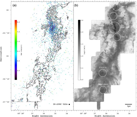
Left: Zeroth moment map of CARMA–NRO 13CO(1–0) (contours) toward Orion A, with SDSS-IN-SYNC YSO positions marked with dots. The colors indicate YSO ages. Right: 13CO(1–0) zeroth-moment map with star-forming clumps studied by Kong et al. (2018) shown by white circles.
2.2 Summary of the CARMA–NRO Orion Survey and methods of analysis for 13CO(1–0)
The CARMA–NRO Orion Survey provides combined 13CO(1–0) data with full-width at half-maximum (FWHM) of the beam ≃ 8″ × 6″, position angle ≃ 10°, channel width ≃0.22 km s−1, and rms noise level ≃ 0.64 K (Kong et al. 2018; see also Nakamura et al. 2019 for the details of the Nobeyama observations). The map spans approximately |${2{^{\circ}_{.}}3}$| along the declination direction covering from OMC-3 (northernmost cloud) to NGC 1999 (southernmost cloud) as shown in the right-hand panel of figure 1.
Here, we take advantage of the high angular resolution of these 13CO(1–0) observations, which is generally sufficient to give independent measurements of gas properties around each YSO in the IN-SYNC survey. We compare the 13CO(1–0) spectra from individual pixels containing IN-SYNC YSO positions to the stellar properties of the corresponding YSOs. There are 1529 YSOs defined as members of Orion A filamentary structure along the declination range of the CARMA–NRO Orion Survey mapping area. Among the IN-SYNC YSOs, 1371 sources are located where the 13CO(1–0) data exist. We investigate all of the 1371 13CO(1–0) spectra and compare them with the YSO properties. We will focus on exploring the physical and kinematic relation between YSOs and the molecular gas (hereafter the gas–YSO association).
Most of the investigated 13CO(1–0) spectra (|$\sim 87\%$|) show multiple velocity components (typically 2–3). We have developed a simple automated metric to determine the number of components and their properties through a multiple-Gaussian-component fitting procedure. For the example spectrum shown in figure 2, we plot the best-fitting reduced χ2 so that |$\chi _{\nu }^2 = [\sum \chi ^2]/{N_{\rm DOF}}$|, where χ2 = [(Tmb, obs − Tmb, exp)/σ]2 for each channel and NDOF (the number of degrees of freedom) = Nchannel − Npar. Tmb, obs is the observed 13CO(1–0) brightness temperature of the channel, Tmb, exp is the expected 13CO brightness temperature of the channel, the total number of channels (Nchannel) is 74, and the number of parameters (Npar) are 3, 6, or 9 (for single, double, or triple Gaussian cases, respectively). We determine the 1σ noise level of the 13CO spectra by examining line-free velocity ranges (typically 0–5 km s−1) of all 1529 sources and derive the median value which is Tmb ∼ 0.59 K. We then select the line emission components over 3σ (Tmb ∼ 1.8 K). The |$\chi _{\nu }^2$| values are compared with single, double, and triple Gaussian models, then the best model is selected that minimizes |$\chi _{\nu }^2$|.
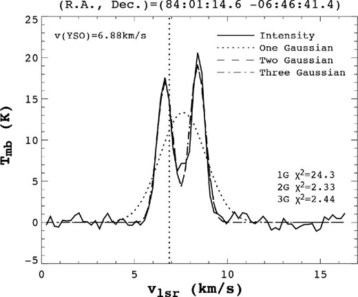
Example 13CO(1–0) spectrum at an IN-SYNC (Da Rio et al. 2016) YSO position with multi-Gaussian fits (RA and Dec at the top of the plot). Solid lines show the observed 13CO(1–0) spectrum. The black dotted, dashed, and long-dashed lines show single, double, and triple Gaussian fits to the spectrum. We select the fiducial multi-Gaussian model from the minimum χ2 values among the models (in this case, two-Gaussian fit). The vertical dotted line indicates the YSO velocity. We derive the σ values of all 1371 spectra (sources in the CARMA–NRO mapping area) and adopt the median value, σ ∼ 0.59 K, to determine the intensity peaks at Tmb ≳ 3σ ∼ 1.8 K.
We compare our 13CO(1–0) fitting method to that of the Semi-automated multi-COmponent Universal Spectral-line fitting Engine (SCOUSE, Henshaw et al. 2016). SCOUSE determines, with user input help, the number of velocity components and their profile information for a given spectrum. We compare peak intensities, widths, and centroids between both methods for 50 selected 13CO spectra. For all of the 50 spectra, our fitting method agrees well with SCOUSE. We note that our method and SCOUSE both utilize MPFIT (a non-linear least-squares fitting method, Markwardt 2009) with the same concepts of NDOF and |$\chi _\nu ^2$|. Thus, it is not surprising to see good agreement between the two methods. We also compare the multi-component fitting models of this study to a PYTHON-based fully automated fitter for multi-component line emissions, the Behind The Spectrum (BTS; Clarke et al. 2018). The difference between SCOUSE and BTS are the input of user-defined parameters where BTS only needs minimal inputs. We show the detail comparison of the derived parameters of the 50 sample spectra with the three different methods in the appendix. The comparison shows that the investigation of the main 13CO(1–0) velocity components of the fitting methods of this study is very robust.
The properties of individual YSOs (age and radial velocity, vYSO; Da Rio et al. 2016) are compared to the major 13CO(1–0) velocity structures (containing the strongest peak) of the corresponding locations (i.e., |$v_{\rm {}^{13}CO}$|): in particular, we examine the difference in radial velocity between the molecular structures as traced by 13CO(1–0) and the YSOs (|$\Delta v=v_{\rm {}^{13}CO}-v_{\rm YSO}$|) at each YSO position. Then, we search for any trend in Δv with YSO age.
2.3 Summary of SOFIA-upGREAT [C ii] data
We utilize a publicly available SOFIA-upGREAT 158 μm [C ii] data set that stems from observations of the northern part of the Orion A cloud (Pabst et al. 2019). The 158 μm SOFIA-upGREAT data have an angular resolution of ∼18″. The [C ii] data cube has a velocity resolution of ∼0.2 km s−1, and an rms noise level of ∼1.0 K (Tmb).
In this work, we perform a qualitative analysis to understand the dynamics of the Orion A region, i.e., whether or not a cloud–cloud collision scenario can be supported. We thus perform normalizations to explore the trends as indicated in figure 3.
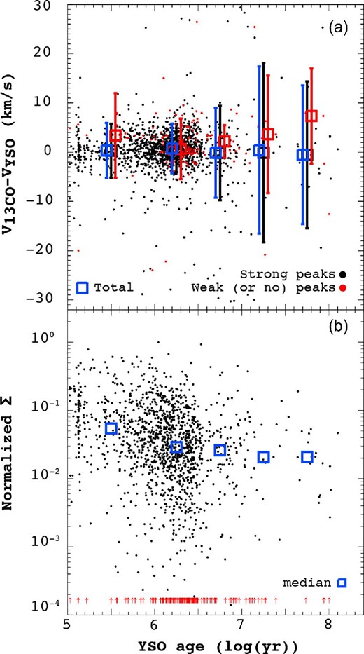
Top: Δv vs. YSO age of Orion A. The black dots are the YSOs where 13CO(1–0) profiles are detected at the pixel position. The red dots are the YSOs with weakly or not detected 13CO(1–0) lines. The average 13CO(1–0) line profile around the pixel position is used for each red dotted YSO. The black, blue, and red boxes indicate the median velocity differences in each YSO age bin (see text for details) for black, red, and all dots, respectively. The velocity differences are derived from the 13CO(1–0) velocity component containing the major peak. Bottom: Σ vs. YSO age of Orion A. The black dots are the same as in the top panel. We normalize the Σ values so that the maximum normalized Σ among the all YSOs in Orion A area is 1. Red upward arrows present the YSO ages of the red dotted data points in the top panel. Blue boxes show the median normalized Σ values of each age bin.
3 Results
3.1 Correlations between gas and YSOs
3.1.1 “Δv vs. age” and “Σ vs. age” of entire Orion A cloud
Figure 1 a shows the location of YSOs on top of the Orion A molecular gas structures. The color of the YSO represents its age (Da Rio et al. 2016), increasing from blue (younger) to red (older). It should be pointed out that YSO ages based on stellar isochrones are quite uncertain, perhaps by a factor of up to 2 (see, for example, the discussions in Vacca & Sandell 2011, Soderblom et al. 2014, and Da Rio et al. 2016). While there is likely to be a minimum uncertainty level of at least 1 Myr in any given absolute age estimate, relative ages are likely to be better determined.
We find that the majority of YSOs with ages ≤1 Myr are located coincident (in projection) with the dense parts of the filamentary molecular structures. On the other hand, older (>1 Myr) YSOs are spread over the entire field. More quantitatively, we determine that |$62\%$| of the younger population (≤1 Myr) is located inside the lowest contour level (30 K km s−1) of the 13CO(1–0) emission, while only |$35\%$| of the relatively older population (>1 Myr) is found inside that contour level. This confirms the expectation that star formation occurs in the densest cloud regions, with the YSOs remaining associated with their natal dense gas for ∼1 Myr, followed by relative motion between stars and gas or gas dispersal after this (see also Da Rio et al. 2016).
Figure 3a shows the difference in velocity between each YSO and its local 13CO(1–0) main component, i.e., Δv, versus YSO age. The black dots are YSOs showing significant 13CO(1–0) emission. The red dots represent those with weak (Tmb < 3σ limit) or no 13CO emission (outside of the mapping area). We use the environmental 13CO intensities which are averaged over the CARMA–NRO beamsize (∼5″) for the weak 13CO sources. The YSOs velocities with no 13CO detection have been compared to the 13CO velocity structures of the main Orion A filament so that we average over 50 pixels (100″) in the Dec direction as well as all pixels in the RA direction. The small boxes in the top left-hand panel of figure 3 indicate the median values of the Δv, and the error bars show the scatters of the data points in each bin. We choose the bin size to be 0.5 dex along the logarithmic YSO ages except for the first bin which includes all YSOs under 1 Myr.
Figure 3b shows the “Σ vs. age” of all YSOs where the mass surface density, Σ, of each source has been derived from the major 13CO component that we use for the “Δv vs. age” relation. As we cannot determine the true environmental Σ for the YSOs without 13CO detection, we do not include them (i.e., red dotted sources in figure 3a) for this analysis. We show the YSO ages of non-detected 13CO(1–0) as red upward arrows (figure 3b).
In figure 3a and table 1, we present the “Δv vs. age” of YSOs that inspects the Δv of the YSOs of age bins ending at 106.0, 106.5, 107.0, 107.5 and 108.0 yr. We first focus on the YSOs within the CARMA–NRO CO mapped area (black colored points in figure 3a, 1371 sources, “Detected” in table 1). These sources show a trend that older YSOs exhibit generally larger scatter in Δv and the median values (black boxes) become more negative in the older population (see table 1). The average values of all YSOs (blue colored points, 1529 sources, “Total” in table 1) present a similar trend to the black points mainly due to their large number which indicates that the IN-SYNC YSOs are mostly associated with the dense molecular structures. The YSOs outside CO maps (red colored points, 158 sources, “Non-detection” in table 1) show a different distribution with Δv values as shown in figure 3a and table 1. The red colored points of figure 3a showing the median Δv values (red boxes) in the age bins become more positive and the scatter gets generally bigger in the older population.
Derived parameters of the gas–YSO association for entire Orion A.
| Age bin (yr) | <106 | 106 to 106.5 | 106.5 to 107.0 | 107.0 to 107.5 | >107.5 | |
|---|---|---|---|---|---|---|
| Detected | Δv (km s−1) | 0.28 | 0.78 | −0.16 | −0.12 | −0.52 |
| σ(Δv) (km s−1) | 5.48 | 4.87 | 9.59 | 18.20 | 14.92 | |
| Normalized Σ | 0.05 | 0.03 | 0.03 | 0.03 | 0.02 | |
| Non-detection | Δv (km s−1) | 3.39 | 0.67 | 2.19 | 3.63 | 7.35 |
| σ(Δv) (km s−1) | 8.60 | 6.16 | 3.33 | 11.95 | 9.67 | |
| Total | Δv (km s−1) | 0.35 | 0.76 | −0.10 | 0.43 | −0.52 |
| σ(Δv) (km s−1) | 5.61 | 5.05 | 9.13 | 16.96 | 14.09 |
The “Σ vs. age” of the entire Orion A is shown in the bottom panel of figure 3, which shows that the younger YSOs are more closely associated with denser gas structures. We normalize the Σ of each YSO position so that the maximum normalized Σ is 1. We find that |$\sim 30\%$| of the YSO population with ages ≤1 Myr have their normalized Σ above 0.1 while |$\sim 12\%$| of the YSOs with ages >1 Myr are above 0.1. The median values of the normalized Σ of the age bins are shown in both figure 3b and table 1. The relatively flat trend for the bins with age ≳ 107 years is possibly due to the small sample size while the normalized Σ decreases along YSO evolution.
3.1.2 “Δv vs. age” and “Σ vs. age” of stellar clusters
In figure 4, we inspect the local trends of six sub-regions corresponding to star clusters (see Kong et al. 2018) marked with white circles in figure 1b. We use the same approach as that performed for the entire Orion A region but consider larger age bin sizes so that we have three bins (age ≤106, 106 > age ≤106.5 and age >106.5 yr). The reason for the reduced number of bins is mainly the small number of YSOs inside the white circles (see table 2 for the number of YSOs in each circle). A typical radius (r ∼ 0.55 pc) is selected from the size of L 1641 N in Nakamura et al. (2012). For convenience, we then apply the same value to all other clusters, except for the ONC-OMC-1 (r ∼ 0.85 pc) which is ∼1.5 times larger than all other regions. The center positions of the clusters are defined by optimal extraction (Naylor 1998) from the 13CO zeroth-moment map produced by Kong et al. (2018). The basic properties of each young stellar cluster are summarized in table 2.
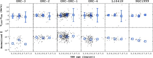
Top: Δv vs. YSO age of each region. Black dots are the YSO sources inside inner circles of figure 3b. The blue boxes show the median Δv of YSOs in three different age bins (age ≤106, 106 > age ≤106.5 and age >106.5 yr). Bottom: Σ vs. age of each region. The blue boxes show the median values of normalized |$\Sigma$| in same age bins.
Observational parameters of stellar clusters in Orion A.
| Source | RA | Dec | |$\widetilde{\Sigma }$| | ||
|---|---|---|---|---|---|
| Source | (hh mm ss.s) | (dd mm ss.s) | r (pc) | NYSO | (g cm−2) |
| ONC–OMC-1 | 5 35 16.6 | −5 22 44.4 | 0.85 | 351 | 0.051 |
| OMC-2 | 5 35 22.4 | −5 07 46.0 | 0.55 | 89 | 0.038 |
| OMC-3 | 5 35 07.6 | −4 55 36.0 | 0.55 | 51 | 0.013 |
| OMC-4 | 5 35 04.8 | −5 35 15.0 | 0.55 | 145 | 0.027 |
| L 1641 N | 5 36 18.8 | −6 22 10.2 | 0.55 | 38 | 0.046 |
| NGC 1999 | 5 36 17.0 | −6 44 20.9 | 0.55 | 25 | 0.025 |
Figure 4 and table 3 show the Δv vs. age and Σ vs. age of the six clusters. The Δv vs. age relation of ONC-OMC-1, OMC-2, OMC-4, and L 1641 N are qualitatively consistent with the trend found for the entire cloud so that median Δv values are close to 0 km s−1 and the scatters increase for the older population. However, OMC-3 and NGC 1999 show different trends to the entire Orion A. The scatters get smaller in the older population, which is possibly due to the small sample size for the old YSO population. The Σ vs. age show that the normalized Σ of ONC–OMC-1, OMC-2, OMC-4, L 1641 N, and NGC 1999 likely decreases while increasing in age, similar to the global trend. The dynamic range of the normalized Σ does not significantly change in OMC-2, L 1641 N, and NGC 1999, i.e., they are different from the global trend, while ONC–OMC-1 and OMC-4 resemble the global trend (having larger dynamic range of Σ in older population). OMC-1 consistently shows a large scatter of the normalized Σ along the YSO ages.
Derived parameters of gas–YSO association for sub-regions.
| Age bin (yr) | <106 | 106 to 106.5 | >106.5 | |
|---|---|---|---|---|
| ONC-OMC-1 | Δv (km s−1) | 0.07 | 1.39 | 1.17 |
| σ(Δv) (km s−1) | 5.20 | 3.30 | 15.58 | |
| Normalized Σ | 0.13 | 0.11 | 0.14 | |
| OMC-2 | Δv (km s−1) | 0.37 | 0.16 | −1.66 |
| σ(Δv) (km s−1) | 3.35 | 3.11 | 8.51 | |
| Normalized Σ | 0.09 | 0.07 | 0.07 | |
| OMC-3 | Δv (km s−1) | −1.73 | −1.30 | −3.70 |
| σ(Δv) (km s−1) | 5.40 | 5.57 | 12.70 | |
| Normalized Σ | 0.01 | 0.03 | 0.01 | |
| OMC-4 | Δv (km s−1) | 0.29 | 0.06 | 0.55 |
| σ(Δv) (km s−1) | 6.89 | 6.32 | 16.38 | |
| Normalized Σ | 0.05 | 0.04 | 0.05 | |
| L 1641 N | Δv (km s−1) | 0.77 | 1.10 | −1.25 |
| σ(Δv) (km s−1) | 1.06 | 2.71 | 13.54 | |
| Normalized Σ | 0.07 | 0.05 | 0.05 | |
| NGC 1999 | Δv (km s−1) | −0.54 | −1.31 | 1.51 |
| σ(Δv) (km s−1) | 2.22 | 2.72 | 1.06 | |
| Normalized Σ | 0.05 | 0.03 | 0.02 |
3.1.3 Probability distribution functions of the velocities
The gas–YSO association along the Orion A filament is investigated via the probability distribution function of vYSO and |$v_{\rm {}^{13}CO}$| (v–PDF). For this analysis, we first divide the Orion A cloud in five regions along declination direction that include defined star clusters, except Region 3 which is located between OMC-4 and L 1641 N. In figure 5, we present the 13CO(1–0) zeroth-moment map showing the five regions on the left and the v–PDFs of the entire Orion A and the five regions on the right. We focus on the positions of the peaks and the FWHM of the distribution functions by performing simple multi-Gaussian fits since sometimes the peak and dispersions do not appear clearly in multi-peaked regions. We investigate the overall trend of the v–PDFs so that the parameters from the Gaussian fits provide us corresponding information. The position of the peaks and the widths of the v–PDF provide the representative velocity structures in the inspected regions and the kinematic dispersion of the them, respectively.
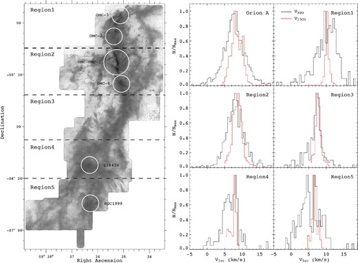
Left: Same as figure 1 (right-hand panel) but overlaying the sub-regions for vYSO vs. |$v_{\rm {}^{13}CO}$| comparison. Right: The histograms of comparing vYSO vs. |$v_{\rm {}^{13}CO}$| of individual pixels possessing YSO locations. The inspected regions (as displayed on the top-right of each panel) correspond to the sub-regions of the 13CO zeroth-moment map while the panel named Orion A presents the histograms for entire Orion A area. The black and red solid lines show vYSO and the |$v_{\rm {}^{13}CO}$|, respectively. We find the width of |$v_{\rm {}^{13}CO}$|–PDF is wider than vYSO–PDF in the norther part of Orion A while the southern part shows a similar width between both PDFs, i.e., Region 3 for the entire vlsr range and Region 4/Region 5 for the peaks around vlsr ∼ 8/6 km s−1. This may indicate the variation of global kinematics along the Orion A filamentary structure.
The v–PDFs of the entire Orion A show single distributions for both vYSO and |$v_{\rm {}^{13}CO}$| where the velocity peaks are separated only by ∼0.4 km s−1. The vYSO distribution is wider than the |$v_{\rm {}^{13}CO}$| distribution while the population of blueshifted YSOs (compared to |$v_{\rm {}^{13}CO}$|) is slightly larger than for the redshifted YSOs. The v–PDF peaks/FWHMs of vYSO and |$v_{\rm {}^{13}CO}$| are ∼8.3|$/$|7.5 km s−1 and ∼8.7|$/$|4.4 km s−1, respectively. There is a second |$v_{\rm {}^{13}CO}$| peak at ∼10.3 km s−1 of the global v–PDF which is dominated by the major |$v_{\rm {}^{13}CO}$| peak of Region 1 that contains OMC-2 and OMC-3 clusters. Region 1 shows a narrow single Gaussian distribution of |$v_{\rm {}^{13}CO}$| where the peak/FWHM is ∼10.7|$/$|0.9 km s−1, while the vYSO shows two relatively wide normal distributions peaked at ∼10.3 (normalized probability ∼0.34) and ∼12.3 km s−1 (normalized probability ∼0.58) with FWHMs of ∼7.3 and 3.1 km s−1, respectively. Region 2 presents mostly blueshifted single Gaussian vYSO distribution. The peak/FWHM of the |$v_{\rm {}^{13}CO}$| and vYSO distributions are ∼9.2|$/$|2.9 km s−1 and ∼8.4|$/$|5.8 km s−1, respectively. Region 3, with no defined active star-forming clumps/clusters, is supposed to be the most quiescent region in Orion A. It shows the most narrow distributions for both |$v_{\rm {}^{13}CO}$| and vYSO. The peak/FWHM values of |$v_{\rm {}^{13}CO}$| are ∼8.2|$/$|0.8 km s−1, and vYSO shows the values as ∼7.9|$/$|1.4 km s−1. The vYSO and |$v_{\rm {}^{13}CO}$| of Region 4 present two distinguished populations. The peak/FWHM values of the vYSO are ∼6.4|$/$|3.3 km s−1 and ∼8.6|$/$|1.0 km s−1 while |$v_{\rm {}^{13}CO}$| show the peaks at ∼6.7 and 8.4 km s−1 for the corresponding FWHMs as ∼1.6 and 0.7 km s−1, respectively. The vYSO and |$v_{\rm {}^{13}CO}$| peaks at ∼6.4 and 6.7 km s−1 are exclusively from the L 1641 N cluster, where the ages of most YSOs inside are smaller than 1 Myr. The Gaussian fits to the v–PDFs of Region 5 show three peaks of vYSO distribution at ∼4.9, 6.7, and 9.6 km s−1 with the FWHMs of 5.8, 0.2, and 2.6 km s−1, respectively. The |$v_{\rm {}^{13}CO}$| distribution shows only one narrow peak at ∼6.9 km s−1 with the FWHM as ∼0.8 km s−1. The normalized |$v_{\rm {}^{13}CO}$| distribution peak of Region 5 is consistent with the ∼6.7 km s−1 peak of vYSO distribution.
3.2 Comparing 13CO(1–0) to [C ii] 158 μm
Bisbas et al. (2018) detected velocity and position offsets between [C ii] 158 μm and 13CO(1–0) line emission maps in IRDC G035.39-00.33. From a comparison with results of numerical models, they claimed that a cloud–cloud collision could explain these offsets, and thus may be a likely formation mechanism for the IRDC. We adopt their methods to test the cloud–cloud collision scenario of star cluster formation in Orion A using the high angular resolution [C ii]158 μm (SOFIA-upGREAT) and 13CO(1–0) (CARMA–NRO) data.
The white circles in figure 6 show the four northern clusters (ONC-OMC-1, OMC-2, OMC-3, and OMC-4) where both the [C ii] and 13CO observations exist as well as two test regions (Edge1 and Edge2). Pabst et al. (2019) inspect the [C ii] PVD of the northern part of Orion A and compare it to a simple model of a spherically expanding shell with a velocity of 13 km s−1. According to their results, the locations of Edge1 and Edge2 can be assumed to be at the border of the expanding shell where the foreground velocity components are either absent or merged into the major peaks. The ONC-OMC-1 region is also consistent with the location of the border of expansion while OMC-4 is situated at the middle of the shell along the line-of-sight direction. The OMC-2 and OMC-3 are outside of the expanding shell, thus we can expect that the gas kinematics on these regions undergo minimal effects of the enormous stellar feedback by θ1 Orionis C (Pabst et al. 2019). The 13CO(1–0) and [C ii] emission from the six sub-regions can thus present the gas kinematics of cold and dense filamentary structures (13CO) or warm envelopes ([C ii]) in different environments with and without effects of strong stellar feedback.
![Map: False-color image showing the zeroth-moment maps of [C ii] (−5.5 ≲ v ≲ 10.0 km s−1, blue), 13CO (green) and [C ii] (10.0 ≲ v ≲ 16.3 km s−1, red). White circles show star-forming regions defined by Kong et al. (2018). Edge1 and Edge2 regions are test regions to compare 13CO vs. [C ii] velocity profiles at the edge of the expanding shell. The numbered crosses indicate randomly selected pixel positions for the 13CO vs. [C ii] velocity comparison. Upper panels: Integrated 13CO (black solid line) and [C ii] (red solid line) velocity profiles inside white circled areas shown in the map. Right-hand panels: Same velocity profiles as in the upper panels but for each randomly selected pixel position marked in the map.](https://oup.silverchair-cdn.com/oup/backfile/Content_public/Journal/pasj/73/Supplement_1/10.1093_pasj_psaa035/3/m_psaa035fig6.jpeg?Expires=1749627205&Signature=mypX86yaLCS-SSH-JM~RLcOzu1cgxOZyyf9PTqxJKN5-uf1dEfhgNCoQ~0Reu1-2W7M13z0U8I9CCHNfRPh1ASTkgJuFXfXipEJnL5KhSi3bMO1LybkrelRcGlDJc0-8qjM-u4BAifokMdx-j81t0EzIiT01wK83H0B-FMp-LawuF6emhT4QBdi9k-hMHNeu6LKFcObIU-TWK-HyYcC6RqqsmX-pGekvjIU77XGqMp6vSlR1GuDKMQsJc1awkjg2GoiVhgcP5tZRtUeeZy41K7WH-P4IUPqSvdIsgP2Mok~9Ahj0fKb1ybPcFAjuH4x2OEe123u4CU0r~8xhCbyMew__&Key-Pair-Id=APKAIE5G5CRDK6RD3PGA)
Map: False-color image showing the zeroth-moment maps of [C ii] (−5.5 ≲ v ≲ 10.0 km s−1, blue), 13CO (green) and [C ii] (10.0 ≲ v ≲ 16.3 km s−1, red). White circles show star-forming regions defined by Kong et al. (2018). Edge1 and Edge2 regions are test regions to compare 13CO vs. [C ii] velocity profiles at the edge of the expanding shell. The numbered crosses indicate randomly selected pixel positions for the 13CO vs. [C ii] velocity comparison. Upper panels: Integrated 13CO (black solid line) and [C ii] (red solid line) velocity profiles inside white circled areas shown in the map. Right-hand panels: Same velocity profiles as in the upper panels but for each randomly selected pixel position marked in the map.
The map of figure 6 shows the false-color zeroth-moment maps of the blueshifted [C ii] (blue), 13CO (green) and redshifted [C ii] (red) emissions. Only the northern part of the 13CO map is covered by the [C ii] SOFIA-upGREAT observation. For the overlap area, we carry out a pixel by pixel velocity comparison between the 13CO and [C ii] lines to search for observational signatures of a cloud–cloud collision. The angular resolution of [C ii] is about three times coarser (∼18″) than that of the 13CO observations (∼8″ × 6″). Thus, we first re-grid the 13CO map to the grid and resolution of the [C ii] data before we perform the velocity comparison. The integrated velocity profiles of 13CO and [C ii] inside the inspected regions (white circles in figure 6) are presented on the upper panels of figure 6. One also needs to note that the wider [C ii] velocity profile than 13CO in all regions only except OMC-4 is possibly due to photoevaporation flows at the surfaces of the denser gas as we know that Orion A is a PDR to a large degree. The nine panels in the right of figure 6 show the 13CO and [C ii] velocity profiles of randomly selected pixel positions (white crosses of figure 6).
The top panels of figure 6 show the integrated line emission (13CO(1–0), black solid line; [C ii], red solid line) inside the six sub-regions. The northernmost cluster, OMC-3, shows two velocity peaks at 11.1|$/$|12.6 km s−1 for 13CO and 11.2|$/$|113.2 km s−1 for [C ii] based on the multi-Gaussian fit. The PVD of the CARMA–NRO 13CO data shows two clear velocity components across the OMC-3 region at ∼11.2 and 12.6 km s−1 (see figure 7). The two velocity components are linked with a prominent “bridge” around (RA, Dec) = (|${5^{\rm h}35^{\rm m}10{^{\rm s}_{.}}0}$|, |$-{04{^\circ }55^{\prime }8{^{\prime \prime}_{.}}8}$|) that is located inside OMC-3. The 13CO and [C ii] emission in OMC-2 shows peak velocities of 10.9 and 10.5 km s−1, respectively. Although both lines have single Gaussian shapes, the FWHM of [C ii] emission is about twice that of the 13CO emission (4.0 vs. 1.9 km s−1). The ONC-OMC-1 cluster shows wide 13CO emission, peaked at 9.7 km s−1 with a FWHM of 3.5 km s−1. The [C ii] emission in ONC-OMC-1 contains two merged velocity components, with peak velocities of vpeak ∼ 5.4 and 9.6 km s−1, and line widths of FWHM ∼10.0 and 4.4 km s−1, respectively. Note that the stronger component is similar to the 13CO emission while the blueshifted weak component is much broader. The weak [C ii] velocity component is assumed to be a result of averaged foreground features of the expanding shell. The OMC-4 region shows clear [C ii] foreground emission associated with the expanding shell at −1.8 km s−1. The 13CO and [C ii] major velocity components are separated only by ∼0.2 km s−1 (vpeak, CO ∼7.6 km s−1 and vpeak, [C ii] ∼ 7.8 km s−1) while the 13CO emission presents additional background features at 10.4 and 12.0 km s−1. The test regions (Edge1 and Edge2) show narrow major 13CO velocity features with broad [C ii] multi-components.
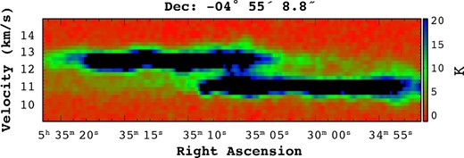
13CO(1–0) PVD of a slice along the RA direction that includes pixel position 5 of figure 6. This PVD shows a clear bridging effect at the position which may indicate a cloud–cloud collision in OMC-3.
One needs to note that Bisbas et al. (2018) predicted position offsets between 13CO and [C ii] emission which are not distinguishable in the integrated line images. The detailed 13CO and [C ii] structures enable us to investigate through a pixel-by-pixel comparison of both line emissions. In the bottom right-hand panels of figure 6, we show the 13CO and [C ii] emissions at nine randomly selected positions that are inside the six sub-regions. This analysis provides an apprehensive idea of the detailed velocity structures and their variations. An extensive pixel-by-pixel comparison with statistical investigation of the 13CO and [C ii] structures of Orion A will be reported in a future paper.
In figure 6, the numbers move from left to right so that the numbers are based on decreasing right ascension. The velocity profile differences between integrated and individual pixel spectra inside each cluster show how averaging spectra smear out significant features. For example, the position of velocity peaks in panel 2 do not match the integrated velocity of the ONC-OMC-1 region. However, all other regions show signs that the global velocity profiles (from clusters) present major and/or minor peaks agreeing with the velocity peaks of individual pixels. The spectral features of panel 1 present similar trends with the integrated emissions of the entire Edge1 area. A narrow 13CO peak is separated only by ∼2 km s−1 from a much wider [C ii] peak while there is a background 13CO emission that does not seem to be connected to the narrow 13CO major peak and has a broader linewidth. Panels 2 (in ONC-OMC-1), 5 (in OMC-3), and 7 (in OMC-4) show qualitatively congruent trends that show two connected velocity components in each 13CO and [C ii] observation where the peak velocities of the two lines agree to within ∼1 km s−1. The most evident case is panel 2. The strongest peaks of the 13CO and [C ii] emission are found at velocities of ∼6.0 and 9.7, respectively, while the secondary peaks are at vpeak, 13CO ∼11.0 km s−1 and |$v_{\rm peak,[C\, {\small II}]} \sim 6.1 \:$|km s−1. Panel 3 shows single Gaussian shapes of 13CO (∼9–13 km s−1) and [C ii] (∼8–14 km s−1). Panels 4 and 6 also show two velocity components in both lines but the main peak of 13CO emission is close to the main [C ii] velocity component. The two peaks are separated by ∼1 km s−1 for panel 4 and ∼1.5 km s−1 for panel 6. The secondary peaks of the [C ii] line are equivalent to the secondary 13CO peaks. The full velocity ranges of [C ii] for both panels 4 and 6 include the 13CO velocity components. Panel 8 shows single Gaussian shapes of 13CO and [C ii] emission but the velocity range of 13CO emission does not completely overlap with the [C ii] emission. The pixel numbered 9 is situated at the edge of the expanding shell (inside Edge2 region). The 13CO emission features of the entire Edge2 region and the pixel numbered 9 quantitatively agree with each other for the peak velocity and the narrow velocity ranges. This may indicate that dense molecular structure in/around the Edge2 area is kinematically quiescent. The [C ii] emission in panel 9 shows a significant secondary feature that is possibly associated with the expanding shell moving toward us, while the integrated [C ii] emission inside the Edge2 region shows a secondary feature which may move away from us. This implies that the warm envelope traced by [C ii] has extreme kinematic variations in/around the Edge2 area compared to the 13CO emission.
4 Discussion
In this study, we present kinematic properties of Orion A by analyzing three independent survey data sets—the SDSS III IN-SYNC, CARMA–NRO ORION 13CO(1–0), and SOFIA-upGREAT 158 μm [C ii] surveys. These observations trace distinct targets and their properties. The IN-SYNC data provide us with the age and radial velocities of YSOs while CARMA–NRO 13CO(1–0) data are sensitive to the gas motion of the coldest and densest parts of molecular structures (e.g., clumps and cores). The SOFIA 158 μm [C ii] fine-structure line measures the energy input into the dense medium possessing insufficient optical depth to shield UV radiation. Here, we discuss the further indication of the analytic results and also compare them to the theoretical models.
4.1 Trends
We have investigated the gas–YSO association in Orion A via analyzing Δv vs. age, Σ vs. age, and v-PDFs of the entire Orion A region as well as for six sub-regions (young stellar clusters). The analysis of the gas–YSO association reveals a trend where dense molecular structures and YSOs lose kinematic adherence with evolution, especially in the northern part of Orion A.
4.2 Comparison with modelling
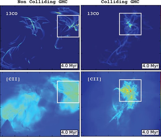
We compare the observational results of gas–YSO associations with those measured from numerical simulations of star cluster formation. To investigate the likelihood of a cloud–cloud collision formation scenario for Orion A, we utilize magnetohydrodynamics (MHD) simulations from Wu et al. (2017a, 2017b), who developed models comparing non-colliding and colliding GMCs. The Wu et al. (2017a) simulations focused on dense molecular structures and synthetic observations. We additionally utilize the Wu et al. (2017b) results which involve modelling of stellar dynamics. Figure 8 presents the snapshots of the simulation 4 Myr after the events (collapsing/colliding) start. Interestingly, the simulated 13CO distribution roughly resembles the global shape of the Orion A molecular cloud, i.e., its filamentary shape with a denser northern part, although the simulation was not intended to reproduce the Orion A cloud. It is worth noting that the off-centered collision preferentially creates such a cloud structure. While MHD simulations of low-mass star-forming regions are capable of producing filamentary structures (e.g., Inoue & Inutsuka 2016), these simulations result in clouds with much lower column density than observed in the Orion A region (by about two orders of magnitude).
![Synthetic line emissions (top: 13CO; bottom: [C ii]) of non-colliding GMCs (left) and colliding GMCs (right) after 4 Myr (Wu et al. 2017a). The white rectangles are the investigated locations for the analyses done in figure 9 and figure 10.](https://oup.silverchair-cdn.com/oup/backfile/Content_public/Journal/pasj/73/Supplement_1/10.1093_pasj_psaa035/3/m_psaa035fig8.jpeg?Expires=1749627205&Signature=IqfW9N-xLRY-U4nY-v9wqkP49ERrkSs8jtX7iFUEBVmhbTHO0Zac61YUqsptyRNsnoz~yTKNEqMrgRlSzjyNAuiLoA1g6xsxIw47YdQyhDpaQ~lVZhj-shKPvQ4vwhcPdi25MC9jyaDT~qCxFsZKNdVDoB9FjXFQ54AEUcLGgMgA1qrUWMaeU0BF0Cpmqrr4speaOa1YJEAJEovgvGFriFDM5-Zeg66ABhGIkdaWLJnuJIgo0LIg-yNBdfk-FFvGYIKd~wbLBXjoxcDARgPlMXGKrzSbveWd1z9ZFRKWdfIJn10p4bHuX4S9TJQsFg7BqnBxjIK2nVn1Jvuc7cMAUQ__&Key-Pair-Id=APKAIE5G5CRDK6RD3PGA)
Figure 9 presents the “Δv vs. age” and “Σ vs. age” relations for the non-colliding and colliding GMCs from the simulated data. The 13CO and [C ii] simulations presented in the current work are derived from Wu et al. (2017a) by post-processing individual snapshots. Using the astrochemical code 3d-pdr1 (Bisbas et al. 2012) and the PDR methodology of connecting the local total H-nucleus number density with a most probable value of effective visual extinction from Bisbas et al. (2017) (see also Wu et al. 2015), we perform synthetic observations of GMC simulations described in Wu et al. (2017a). The white rectangles in figure 8 show the location where we extract the data points (their size is ∼16 × 16 pc2; note that the entire CARMA–NRO Orion survey field is ∼16 pc; Kong et al. 2018). We find that the cloud–cloud collision scenario reproduces the gas–YSO association of the entire Orion A qualitatively better (cf. figure 3; |$\widetilde{\Delta v} \sim$| 0 km s−1, larger Δv scatter at older population, decreasing |$\widetilde{\Sigma }$| along evolution, and larger Σ scatter at older population) when compared to the non-colliding scenario. It should be noted that the numerical codes underestimate the increasing Δv scatter of the YSOs since the spatial resolution of the simulations are not enough to resolve the close encounters (Wu et al. 2017b). Thus, the models provide lower limits but the qualitative results, i.e., the trends, shown here should be met. The non-colliding GMC model shows that the stars are consistently well-associated with the dense molecular clouds, thus no active dispersion happens, while the cloud–cloud collision generates large dispersion throughout its dynamical evolution. These simulated trends are consistent for different projections as seen in figure 9.
Top: Simulated “Δv vs. age” of non-colliding GMC (left) and colliding GMC (right). The results of different projects are displayed in red (X), blue (Y), and black (Z). Bottom: Same as the top plots but for normalized Σ vs. age.
As seen in figure 4, ONC-OMC-1 and OMC-4 clusters show the clearest trends resembling the colliding GMC cases while OMC-2 arguably favors the cloud–cloud collision scenario only from the trend of Δv vs. age. The trends for OMC-3 are very different from any other sub-regions showing smaller Δv vs. age scatter for the older population and a large scatter in Σ vs. age without any specific trend. This could indicate a young dynamic age of the region where two or more star-forming clouds are interacting, merging, and thereby triggering more star-formation. The NGC 1999 region is relatively quiescent and more consistent with the non-colliding GMC case. On the other hand, L 1641 N shows a trend of Δv vs. age that is more consistent with the cloud–cloud collision scenario while the tendency of Σ vs. age is unclear.
The possibility of cloud–cloud collision in the northern part of Orion A is collated by comparing the observed line profiles of the 13CO and [C ii] emission to theoretical models based on Bisbas et al. (2018). In particular, we focus on sub-regions within non-colliding and colliding clouds at dynamical times of t = 4 Myr (see also Bisbas et al. 2018) containing dense filaments and we perform radiative transfer calculations for the lines of [C ii] 158 μm and 13CO(1–0) (covering the white rectangles in figure 9). To obtain the level populations of 13CO, we assume an isotopologue abundance ratio of 12CO/13CO = 60, close to the value of 69.6 used in subsection 2.2. It can be seen that there is a velocity offset between the peaks of these two emission lines, indicating a cloud–cloud collision scenario in agreement with Bisbas et al. (2018) who performed detailed, full 3D simulations in a similar case.
The panels entitled “NCC”, “CC90”, and “CC” in figure 10 show the [C ii] and 13CO spectra of non-colliding clouds, colliding clouds from an edge-on view, and colliding clouds from a face-on view, respectively. NCC shows single Gaussian profiles for both lines, with small velocity offsets which can be associated with turbulent motions in a self-gravitationally collapsing cloud. The CC model shows a clear offset between 13CO and [C ii] main velocity peaks while the linewidth of [C ii] embraces 13CO in both CC and CC90 cases. The densest part of merging clouds can be traced at the major 13CO peak while the [C ii] lines may trace the envelopes around the merging interface. CC90 shows complicated features which can naturally arise from the turbulent motion of the gas. We summarize the observational signals of cloud–cloud collision by the 13CO vs. [C ii] comparison as follows. The trends between position and velocity offsets observed in Orion A (see figure 6) are similar to those suggested in Bisbas et al. (2018). In addition, a [C ii] linewidth larger than the 13CO one where the [C ii] covers the entire 13CO line (we refer to this as [C ii] embracing) suggest a cloud–cloud collision scenario.
![Synthetic 13CO (black solid line) and [C ii] (red solid line) velocity profiles based on the simulations shown in figure 8. The panels named “NCC”, “CC90”, and “CC” represent the simulation results (based on Bisbas et al. 2018) of non-colliding clouds, colliding clouds with an edge-on view, and colliding clouds with a face-on view, respectively. These profiles are extracted from a thin slice for each case representing the local conditions at the densest region of the cloud (see section 4 for detail).](https://oup.silverchair-cdn.com/oup/backfile/Content_public/Journal/pasj/73/Supplement_1/10.1093_pasj_psaa035/3/m_psaa035fig10.jpeg?Expires=1749627205&Signature=t0UGCOb2yoqXJ78QSwVk42axQC6cc-kKbEF2dKitvkkVUpspFbv1IaExbN2~825J7Cf9666cUYIDuUH8~PP-Rdt417IgtBCWra95jIVzXBD~AlANOmoq71tD4vhbhd8nd2gHEQ8XA1BC0Ln~XGc38kDvdQDY27rX7BJxYfs4JsM5utPWgECGlEf3Swa2bFzKwHNJgxMeSEebBxNt4skfn9S1h0GJ-AFEBTXZZfDCnTJmSO6Xp1sZ5aeEG3AjanxCA6anVHotoZhDI-BbKeM9n0U7XZyf9KX95Ntnr6UKJqfVDhyFteh-HNUOJ7EPmVwELxKE2K3TlpVlHTp3fjQQKA__&Key-Pair-Id=APKAIE5G5CRDK6RD3PGA)
Synthetic 13CO (black solid line) and [C ii] (red solid line) velocity profiles based on the simulations shown in figure 8. The panels named “NCC”, “CC90”, and “CC” represent the simulation results (based on Bisbas et al. 2018) of non-colliding clouds, colliding clouds with an edge-on view, and colliding clouds with a face-on view, respectively. These profiles are extracted from a thin slice for each case representing the local conditions at the densest region of the cloud (see section 4 for detail).
The spectra from the theoretical models were extracted from a 2-pc-wide strip across the densest part of the cloud for each colliding scenario as well as along the line of sight (Bisbas et al. 2018). The entire simulated cloud structure has an effective radius of reff ≳ 20 pc so the strip is considered as a thin slice of the cloud. As the “thin slice” represents the local environment of each scenario, the proper observational analogue would be to analyze individual spectral pixels rather than the averaged spectra of an entire cluster. This aspect is presented in the upper panel of figure 6. The integrated 13CO and [C ii] line profiles do not show clear trends of cloud–cloud collision in any of the northern sub-regions, except the larger [C ii] linewidth, compared to the 13CO linewidth, in OMC-1–ONC, OMC-2, and OMC-3 regions. The line profiles of individual pixel positions provide hints of non-colliding and/or colliding GMC scenarios in different regions. Panels 2, 3, 4, 5, and 6 show consistency with the CC model, while panels 7 and 8 arguably show single Gaussian profiles for both 13CO and [C ii] with certain velocity offsets without the [C ii] embracing which may favor of the NCC model. The velocity profiles of shell locations 1 and 9 resemble the integrated line emission of the entire test regions. Based on the analytic results, we assume that the cloud–cloud collision in the northern part of Orion A may be an important mechanism for the ongoing star cluster formation. This is consistent with an ammonia line survey toward the cores of Orion A cloud by Kirk et al. (2017). They found that most cores are not gravitationally bound but created and stabilized by external pressure. One needs to note that such a mechanism can be also triggered by expending PDR shells located near to the OMC-3 region. A well-known expanding bubble, NGC 1977, is located close to the northern direction of OMC-3. A more extended analysis of the pixel-by-pixel 13CO vs. [C ii] comparison will help to statistically confirm or refute the cloud–cloud collision scenario in the Orion A region in a forthcoming work.
4.3 Concluding remarks
We have investigated the kinematic properties of various structures in the Orion A cloud in order to examine the star cluster formation mechanisms. Even with the qualitatively consistent observational evidence of cloud–cloud collision as an important star-cluster-forming mechanism in Orion A, one needs further interpretation of this as the dominant process of the star cluster formation. Similar to Feddersen et al. (2019) and Pabst et al. (2019), we find that the kinematic contribution of stellar feedback in Orion A is significant enough to affect the entire system where the feedback from OB association can even create the Orion A filament (Bally et al. 1987). For instance, the gas around the older YSOs could have been dispersed by external processes or feedbacks so that the loosening gas–YSO association is generated by such mechanisms. Because the simulations do not contain stellar feedback, the theoretical models including strong stellar feedback are needed to confirm the observational evidences of cloud–cloud collision. The large structure dynamics involving multiple molecular structures can include, but is not limited to, gravitational converging flows from a rotating sheet (Hartmann & Burkert 2007), and the oscillating dense filamentary structures which can eject star system from the mother clouds—the so-called slingshot mechanism (Stutz & Gould 2016). These scenarios can explain the larger Δv scatter at older YSO populations by the global motions of the molecular clouds but are unable to address the velocity offset between the 13CO and [C ii] emission. With careful investigations involving the large-scale dynamics with various levels of stellar feedback input, we will be able to have more complete understanding about what observations tell us about the Galactic star cluster formation processes.
Acknowledgements
The authors thank an anonymous referee for constructive comments that help to improve the manuscript. The authors also thank B.-G. Andersson, H. Arce, J. Carpenter, J. Jackson, T. Le Ngoc, W. Reach, A. Soam, and W. Vacca for helpful discussions. WL acknowledges supports from SOFIA Science Center. This work is based on observations made with the NASA/DLR Stratospheric Observatory for Infrared Astronomy (SOFIA). SOFIA is jointly operated by the Universities Space Research Association, Inc. (USRA), under NASA contract NAS2-97001, and the Deutsches SOFIA Institut (DSI) under DLR contract 50 OK 0901 to the University of Stuttgart. GREAT, used for the [C ii] observations, is a development by the MPI für Radioastronomie and the KOSMA / Universität zu Köln, in cooperation with the MPI für Sonnensystemforschung and the DLR Institut für Planetenforschung. Part of this research was carried out at the Jet Propulsion Laboratory, California Institute of Technology, under a contract with the National Aeronautics and Space Administration. This work was carried out as one of the large projects of the Nobeyama Radio Observatory (NRO), which is a branch of the National Astronomical Observatory of Japan, National Institute of Natural Sciences. We thank the NRO staff for both operating the 45 m and helping us with the data reduction. This work was financially supported by Grant-in-Aid for Scientific Research (Nos. 17H02863, 17H01118).
Appendix 1 Comparing multi-component Gaussian fitters
In this section, we introduce the derived parameters of the three different multi-component line fitters of this study, SCOUSE, and BTS. In table 4 and figure 11, we present the parameters of the main components only with the number of components each fitter derived. As shown in figure 11, we compare the three Gaussian parameters, i.e. the peak intensities, central velocities, and FWHMs of the main components, among the fitters while we use the parameters of this study as the references. The 42 out of 50 sample YSOs show that the peak intensities of BTS and/or SCOUSE agree within 2 K. The other 8 sources show that both BTS and SCOUSE agree each other for the peak intensities within 2 K while they differ from the intensities from this study by ∼3–12 K. The FWHMs also vary by about a factor of two at the most extreme case. The central velocities are agreeing quite well (all within 1 km s−1) so that our main point, investigating the difference in the velocities, is very robust.
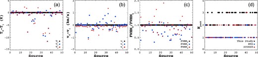
Comparisons of the parameters derived from the three different multi-Gaussian fitters. As for table 4, we focus only on the parameters of the main peaks. Panel (a) shows the comparison of peak temperatures of the fitters. T0 (black dots) indicates the peak temperature from the Gaussian fitter of this study. T1 (blue dots) and T2 (red dots) represent the peak temperatures of BTS and SCOUSE, respectively. Panels (b) and (c) are the same as panel (a) but for the comparisons of the central velocities and FWHMs. Panel (d) shows the number of peaks from the three methods.
Derived parameters of the multi-Gaussian fits to 50 randomly selected sources.
| This study | BTS | SCOUSE | ||||||||||
|---|---|---|---|---|---|---|---|---|---|---|---|---|
| Source | Npeak | Tpeak | vpeak | FWHM | Npeak | Tpeak | vpeak | FWHM | Npeak | Tpeak | vpeak | FWHM |
| (K) | (km s−1) | (km s−1) | (K) | (km s−1) | (km s−1) | (K) | (km s−1) | (km s−1) | ||||
| 1 | 2 | 12.93 | 7.28 | 1.00 | 2 | 13.28 | 7.88 | 2.57 | 1 | 13.02 | 7.38 | 0.76 |
| 2 | 2 | 16.64 | 6.85 | 1.53 | 1 | 16.41 | 6.87 | 1.60 | 1 | 16.41 | 6.98 | 1.60 |
| 3 | 3 | 18.81 | 6.94 | 1.09 | 1 | 18.19 | 6.83 | 1.39 | 2 | 19.22 | 7.02 | 1.13 |
| 4 | 1 | 17.93 | 6.77 | 1.34 | 1 | 17.93 | 6.77 | 1.34 | 1 | 17.93 | 6.89 | 1.34 |
| 5 | 2 | 17.93 | 6.96 | 1.35 | 1 | 17.80 | 6.93 | 1.44 | 1 | 17.80 | 7.04 | 1.44 |
| 6 | 2 | 18.77 | 6.95 | 1.07 | 1 | 18.18 | 6.83 | 1.39 | 1 | 18.18 | 6.94 | 1.38 |
| 7 | 3 | 6.08 | 6.60 | 2.81 | 1 | 7.02 | 6.59 | 2.76 | 1 | 7.02 | 6.70 | 2.76 |
| 8 | 2 | 16.79 | 6.92 | 1.46 | 1 | 16.64 | 6.93 | 1.48 | 1 | 16.64 | 7.04 | 1.49 |
| 9 | 2 | 5.92 | 4.17 | 1.00 | 1 | 6.21 | 4.18 | 0.94 | 2 | 6.30 | 4.28 | 0.88 |
| 10 | 2 | 17.01 | 6.93 | 1.43 | 1 | 16.89 | 6.94 | 1.46 | 1 | 16.89 | 7.05 | 1.46 |
| 11 | 1 | 21.09 | 8.00 | 1.77 | 1 | 21.09 | 8.00 | 1.77 | 1 | 21.09 | 8.11 | 1.77 |
| 12 | 2 | 5.13 | 14.21 | 2.11 | 1 | 4.81 | 14.09 | 2.64 | 2 | 4.96 | 14.37 | 1.91 |
| 13 | 3 | 4.15 | 7.84 | 3.84 | 1 | 4.57 | 8.86 | 5.37 | 1 | 4.57 | 8.97 | 5.36 |
| 14 | 3 | 23.72 | 10.29 | 1.00 | 1 | 7.89 | 9.51 | 3.20 | 2 | 21.54 | 10.42 | 0.74 |
| 15 | 1 | 4.07 | 9.45 | 4.50 | 1 | 4.07 | 9.45 | 4.50 | 1 | 4.07 | 9.56 | 4.50 |
| 16 | 1 | 7.88 | 10.41 | 3.16 | 1 | 7.88 | 10.41 | 3.16 | 2 | 6.18 | 10.83 | 1.95 |
| 17 | 3 | 27.85 | 11.33 | 1.00 | 1 | 35.66 | 11.63 | 1.44 | 1 | 35.66 | 11.75 | 1.44 |
| 18 | 2 | 20.56 | 7.61 | 1.00 | 1 | 21.59 | 7.95 | 1.65 | 1 | 21.59 | 8.06 | 1.65 |
| 19 | 2 | 13.49 | 8.56 | 1.00 | 2 | 14.38 | 8.54 | 0.89 | 2 | 14.38 | 8.65 | 0.91 |
| 20 | 1 | 3.78 | 9.28 | 4.15 | 1 | 3.78 | 9.28 | 4.14 | 1 | 3.78 | 9.39 | 4.15 |
| 21 | 3 | 19.41 | 10.43 | 1.00 | 1 | 22.89 | 10.29 | 1.55 | 2 | 19.85 | 10.52 | 0.90 |
| 22 | 3 | 13.94 | 9.35 | 1.00 | 1 | 16.89 | 9.42 | 1.81 | 1 | 16.89 | 9.53 | 1.82 |
| 23 | 2 | 12.01 | 9.43 | 2.67 | 1 | 15.44 | 9.69 | 2.47 | 3 | 16.46 | 10.24 | 1.42 |
| 24 | 3 | 26.26 | 11.44 | 1.49 | 1 | 28.82 | 11.19 | 2.07 | 2 | 30.52 | 11.49 | 1.54 |
| 25 | 1 | 11.82 | 9.58 | 2.88 | 1 | 11.82 | 9.58 | 2.87 | 1 | 11.82 | 9.69 | 2.88 |
| 26 | 3 | 28.98 | 10.95 | 2.01 | 1 | 29.34 | 10.94 | 2.12 | 1 | 29.34 | 11.05 | 2.13 |
| 27 | 3 | 9.45 | 10.40 | 1.77 | 1 | 9.13 | 9.91 | 3.20 | 2 | 7.53 | 10.76 | 1.62 |
| 28 | 2 | 8.81 | 8.52 | 1.05 | 2 | 8.75 | 8.52 | 1.07 | 2 | 8.75 | 8.63 | 1.07 |
| 29 | 3 | 4.43 | 13.27 | 1.47 | 1 | 4.14 | 12.51 | 3.79 | 2 | 4.80 | 13.23 | 1.82 |
| 30 | 3 | 3.66 | 10.75 | 1.15 | 1 | 3.56 | 10.56 | 2.94 | 2 | 3.61 | 10.81 | 2.62 |
| 31 | 2 | 28.21 | 7.94 | 3.36 | 1 | 28.44 | 7.81 | 3.58 | 2 | 28.25 | 8.04 | 3.38 |
| 32 | 2 | 19.52 | 10.38 | 1.45 | 1 | 28.70 | 9.47 | 2.45 | 2 | 28.01 | 9.05 | 1.43 |
| 33 | 2 | 22.21 | 9.17 | 3.08 | 1 | 23.19 | 9.52 | 3.60 | 1 | 23.19 | 9.63 | 3.60 |
| 34 | 3 | 9.48 | 8.86 | 1.91 | 1 | 18.94 | 9.25 | 3.04 | 2 | 17.69 | 9.19 | 2.94 |
| 35 | 2 | 6.22 | 8.32 | 1.56 | 1 | 5.42 | 8.00 | 2.57 | 2 | 6.15 | 8.40 | 1.65 |
| 36 | 3 | 22.46 | 8.95 | 1.19 | 1 | 34.01 | 9.26 | 1.86 | 1 | 34.01 | 9.38 | 1.87 |
| 37 | 3 | 15.99 | 7.74 | 1.62 | 2 | 22.33 | 7.83 | 2.00 | 2 | 22.33 | 7.94 | 1.99 |
| 38 | 3 | 25.96 | 7.88 | 1.31 | 1 | 25.97 | 7.88 | 1.32 | 1 | 34.31 | 7.67 | 2.11 |
| 39 | 2 | 19.06 | 9.33 | 1.00 | 1 | 20.11 | 8.65 | 2.31 | 2 | 17.47 | 9.50 | 0.85 |
| 40 | 3 | 11.49 | 5.68 | 1.13 | 2 | 12.94 | 6.18 | 1.91 | 3 | 12.55 | 6.02 | 1.45 |
| 41 | 2 | 25.83 | 9.03 | 3.25 | 2 | 26.23 | 9.11 | 3.36 | 3 | 26.29 | 9.57 | 2.41 |
| 42 | 2 | 20.11 | 9.08 | 1.39 | 1 | 20.11 | 9.08 | 1.39 | 1 | 20.11 | 9.19 | 1.39 |
| 43 | 2 | 8.28 | 7.05 | 2.26 | 2 | 8.26 | 7.16 | 2.51 | 2 | 8.26 | 7.27 | 2.51 |
| 44 | 3 | 14.33 | 10.68 | 1.10 | 1 | 15.04 | 10.67 | 1.30 | 1 | 15.04 | 10.78 | 1.28 |
| 45 | 2 | 14.20 | 9.08 | 1.18 | 1 | 13.89 | 9.05 | 1.27 | 1 | 13.89 | 9.16 | 1.27 |
| 46 | 3 | 9.16 | 8.37 | 2.40 | 2 | 9.10 | 8.41 | 2.34 | 2 | 9.10 | 8.52 | 2.34 |
| 47 | 1 | 20.27 | 8.27 | 1.98 | 1 | 20.27 | 8.27 | 1.98 | 1 | 20.27 | 8.38 | 1.98 |
| 48 | 3 | 10.87 | 8.40 | 1.69 | 1 | 10.16 | 8.33 | 2.03 | 2 | 10.88 | 8.52 | 1.68 |
| 49 | 3 | 9.90 | 8.53 | 1.98 | 2 | 9.90 | 8.54 | 1.95 | 2 | 9.90 | 8.65 | 1.95 |
| 50 | 3 | 7.21 | 8.09 | 1.31 | 1 | 7.89 | 8.05 | 2.57 | 1 | 7.89 | 8.16 | 2.57 |
The fitter of this study tends to have more number of peaks than BTS and SCOUSE. This is mainly due to their approaches to multi-components having close central velocities. The multi-Gaussian fitter of this study assumes that such close components are results of very close gas structures while BTS and SCOUSE sometimes assume those as results of self-absorption lines. This can also explain the several of the much higher intensity peaks in BTS and SCOUSE than those of this study. One needs to note that we use 13CO(1–0) emission line which is optically thin in general where the effects of self-absorption are rare.
