


Abstract
Herein, we present results from observations of the 12CO (J = 1–0), 13CO (J = 1–0), and 12CO (J = 2–1) emission lines toward the Carina nebula complex (CNC) obtained with the Mopra and NANTEN2 telescopes. We focused on massive-star-forming regions associated with the CNC including the three star clusters Tr 14, Tr 15, and Tr 16, and the isolated WR-star HD 92740. We found that the molecular clouds in the CNC are separated into mainly four clouds at velocities −27, −20, −14, and −8 km s−1. Their masses are 0.7 × 10⁴ M⊙, 5.0 × 10⁴ M⊙, 1.6 × 10⁴ M⊙, and 0.7 × 10⁴ M⊙, respectively. Most are likely associated with the star clusters, because of their high 12CO (J = 2–1)/12CO (J = 1–0) intensity ratios and their correspondence to the Spitzer 8 μm distributions. In addition, these clouds show the observational signatures of cloud–cloud collisions. In particular, there is a V-shaped structure in the position–velocity diagram and a complementary spatial distribution between the −20 km s−1 cloud and the −14 km s−1 cloud. Furthermore, we found that SiO emission, which is a tracer of a shocked molecular gas, is enhanced between the colliding clouds by using ALMA archive data. Based on these observational signatures, we propose a scenario wherein the formation of massive stars in the clusters was triggered by a collision between the two clouds. By using the path length of the collision and the assumed velocity separation, we estimate the timescale of the collision to be ∼1 Myr. This is comparable to the ages of the clusters estimated in previous studies.
1 Introduction
1.1 Massive star formation
Massive stars are influential in the galactic environment, because they release heavy elements and large amounts of energy in the form of ultraviolet radiation, stellar winds, outflows, and supernova explosions. It is therefore of fundamental importance to understand the formation mechanisms of massive stars, and considerable efforts have been made to date (e.g., Wolfire & Cassinelli 1987; Zinnecker & Yorke 2007; Tan et al. 2014). Most remarkably, recent observational studies have increasingly revealed the importance of cloud–cloud collisions (CCCs). The recent successful development of observational tools for identifying CCCs—i.e., the complementary spatial distributions and bridging features between the colliding clouds—has enabled us to create a firm basis for studying them (e.g., Fukui et al. 2018). When two clouds collide, one burrows into the other as a result of momentum conservation (Haworth et al. 2015). As a simple example, if a collision takes place head-on between two clouds of different sizes, a cavity will be formed in the larger one through this process, and the larger cloud will appear as a ring-like structure on the plane of the sky, unless the observer’s viewing angle is perfectly perpendicular to the collision axis. As the size of the cavity corresponds to that of the smaller cloud, an observer with a viewing angle parallel to the collision axis sees a complementary distribution between the smaller cloud and the ring-like structure. The bridging feature is relatively weak CO emission at intermediate velocities between the two colliding clouds, which are separated in the position–velocity (p–v) diagram. When one cloud collided with another, a dense compressed and turbulent layer is formed at the collision interface. If one observes a snapshot of this collision at a viewing angle parallel to the collision axis, two velocity peaks separated by intermediate-velocity emission with lower intensity are seen in the p–v diagram. The turbulent gas that creates the bridging feature can be replenished as long as the collision continues. Many observational studies have reported detections of such complementary spatial distributions and bridging features in CCC regions (e.g., Enokiya et al. 2018; Fujita et al. 2019, 2021a, 2021b; Fukui et al. 2014, 2016, 2017a, 2019; Furukawa et al. 2009; Hayashi et al. 2018; Kohno et al. 2018; Ohama et al. 2010; Sano et al. 2018; Tokuda et al. 2019; Torii et al. 2015, 2017a, 2017b, 2018, 2019, 2021). The p–v diagram of the colliding clouds exhibits a V-shaped structure that depends upon the conditions such as the viewing angle and cloud sizes.
1.2 The Carina nebula complex
The Carina nebula complex (CNC) and Gum 31 are located in the Carina spiral arm (e.g., Vallée 2014), and the CNC is one of the most active massive-star-forming regions in the Milky Way. Approximately 140 massive OB-stars (Alexander et al. 2016) and more than 1400 young stellar objects (Povich et al. 2011) have been identified in the CNC. The distance to the CNC, ∼2.3 kpc, has been measured accurately by near-infrared spectroscopy observations (e.g., Allen & Hillier 1993; Smith 2006a). We adopt this value in this paper. The number of O-stars in the CNC is comparable to that in other active massive-star-forming regions in the Milky Way, such as W 43 and W 51 (e.g., Blum et al. 1999; Okumura et al. 2000), but the CNC is two or three times nearer than those regions (e.g., Zhang et al. 2014; Sato et al. 2010). Therefore, the CNC offers unique observational advantages for studies of massive-star formation. To date, observations of CO emission covering the entire region of the CNC have been conducted. The 12CO (J = 1–0) map obtained with the Mopra Telescope by Brooks et al. (1998) achieved a 45″ resolution. Subsequently, maps of 3′–4′ resolution have been obtained for the 12CO (J = 1–0), 13CO (J = 1–0), and C18O (J = 1–0) emission lines using the NANTEN telescope (Yonekura et al. 2005). Most recently, Rebolledo et al. (2016) reported column densities for the molecular clouds associated with the CNC and Gum 31 by using the high-resolution 12CO and 13CO (J = 1–0) emission data obtained with Mopra. They found regional variations in the column densities obtained from the fraction of the mass recovered from the CO emission lines relative to the total mass traced by the dust emission. However, the velocity structures of the associated clouds have not previously been analyzed in detail.
Figure 1a shows a composite-color image of the WISE 22 μm (red) and Spitzer/GLIMPSE 8 μm (green) emissions around the CNC and Gum 31. The 22 μm emission, which traces mainly hot dust from H ii regions, extends over ∼50 pc through the CNC, and the data near the center of the CNC [|$(l, b)=({287{_{.}^{\circ}}5}, -{0{_{.}^{\circ}}6})$|] are saturated. On the other hand, Gum 31 is relatively small and resembles the Spitzer bubbles (Churchwell et al. 2006, 2007), although the radius is somewhat larger (∼10 pc) than is typical for those bubbles. In this paper, we focus on the area outlined by the black rectangle in figure 1b, which includes the star clusters Trumpler 16 (Tr 16), Trumpler 14 (Tr 14), and Trumpler 15 (Tr 15). We will focus on Gum 31 in a forthcoming paper (paper II of this series).
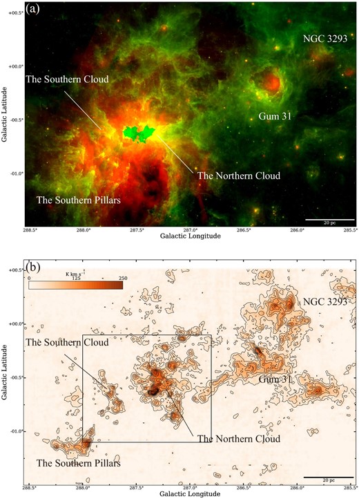
(a) Composite-color image of the WISE 22 μm (red) and Spitzer/GLIMPSE 8 μm (green) emissions around the CNC and Gum 31. (b) Integrated-intensity map of the 12CO (J = 1–0) emission taken from the Mopra archive (Rebolledo et al. 2016, 2017) between the velocities of −35 and 0 km s−1. The black contours are plotted every 25 K km s−1 from 25 K km s−1 (∼10σ). The black rectangle outlines the area shown in figure 2. (Color online)
2 Dataset
2.1 Mopra
We used the 12CO and 13CO (J = 1–0) archived datasets obtained with the Mopra 22 m telescope (Burton et al. 2013; Braiding et al. 2015; Rebolledo et al. 2016, 2017). The beam size and velocity resolution are ∼35″ and ∼0.09 km s−1, respectively. The typical rms noise levels for the 12CO and 13CO (J = 1–0) datasets at a velocity grid of 0.09 km s−1 are ∼4.0 K and ∼1.9 K per channel on the Tmb scale. Details of the observations, calibration, and data reduction are summarized in Burton et al. (2013).
2.2 NANTEN2
The 12CO (J = 2–1) observations were made using the NANTEN2 4 m millimeter/sub-millimeter telescope at Atacama, Chile in 2015 October. The half-power beam-width of NANTEN2 at ∼230 GHz corresponds to ∼90″, and we adopted the on-the-fly (OTF) mapping mode with Nyquist sampling. The 12CO (J = 2–1) emissions were obtained with the 4 K cooled Nb SIS DSB mixer receiver, with a typical system noise temperature including the atmosphere of 300–440 K. A Fourier digital spectrometer installed on the backend of the beam transmission system provides data resolved into 16384 channels at 1 GHz bandwidth. We smoothed them to a velocity grid of 0.5 km s−1. We summed up two orthogonal scan maps (the galactic longitude-scan and the galactic latitude-scan maps) with 15′ × 15′ binning to reduce scanning effects. A typical uncertainty in the intensity is |$\sim 20\%$|. We determined the scaling factor used to convert the intensities to absolute intensities from pixel-by-pixel comparisons between the 12CO (J = 2–1) maps obtained with NANTEN2 (|$T_{\rm a}^{*}$|) and with the 1.85 m telescope (Tmb) toward Orion B (Onishi et al. 2013; Nishimura et al. 2015). The typical rms noise level for the 12CO (J = 2–1) data at the velocity grid of 0.5 km s−1 is ∼0.3 K per channel on the Tmb scale.
2.3 ALMA
We used the SiO (v = 0, J = 2–1) at 86.84696 GHz and H13CO+ (J = 1–0) at 86.75428 GHz of the ALMA 7 m array archived datasets. The observations were conducted during the ALMA Cycle 4 under the project code 2016.1.01609.S (Rebolledo et al. 2020). The beam size and velocity resolution are ∼15″ and ∼0.5 km s−1, respectively, at the final data cube. The details of the observations are described in Rebolledo et al. (2020).
3 Results
3.1 Large-scale gas distributions
Figure 1b shows the integrated-intensity distributions of the 12CO (J = 1–0) emission obtained with the Mopra telescope in the velocity range from −35 to 0 km s−1. Figure 2 shows a close-up version that includes the massive stars listed by Hamann, Gräfener, and Liermann (2006) and Alexander et al. (2016). The detected clouds can be separated mainly into a northern part and a southern part. Rebolledo et al. (2016) called these the Northern Cloud and the Southern Cloud, respectively. The Northern Cloud may be associated with the star clusters Tr 14 and Tr 15. The isolated WR-star HD 92740 is also associated with the Northern Cloud. On the other hand, the center of Tr 16 is located between the Northern Cloud and the Southern Cloud.

3.2 Velocity structures and CO ratio
Figure 3 shows the v–b diagrams of the 12CO (J = 1–0) emission toward the Southern Cloud (figure 3a) and the Northern Cloud (figure 3b), respectively. The main component of the Southern Cloud has velocities of −30 to −20 km s−1, and relatively weak emissions were also detected at ∼−20 km s−1 and ∼−14 km s−1 at |$b=\,{\sim}{-0{{_{.}^{\circ}}}080 }$| and |$-{0{{_{.}^{\circ}}}055 }$|. In contrast, the velocity structure of the Northern Cloud consists of several components ranging from ∼−30 km s−1 to ∼−5 km s−1, as shown in figure 3b. We identified four clouds separated in velocity and centered at −27, −20, −14, and −8 km s−1 (hereinafter called the −27 km s−1 cloud, the −20 km s−1 cloud, the −14 km s−1 cloud, and the −8 km s−1 cloud, respectively). Clear self-absorption features are not found anywhere in the region.
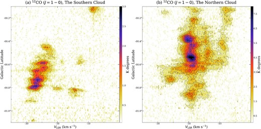
(a) Velocity–galactic latitude (v–b) diagram of the 12CO (J = 1–0) emissions from the Southern Cloud integrated from |${287{_{.}^{\circ}}88}$| to |${287{_{.}^{\circ}}58}$|. The black contours are plotted at every 0.56 K from 0.56 K (∼10σ). (b) Velocity–galactic latitude (v–b) diagram of the 12CO (J = 1–0) emission from the Northern Cloud integrated from |${287{_{.}^{\circ}}55}$| to |${286{_{.}^{\circ}}95}$|. The black contours are plotted every 0.78 K from 0.78 K (∼10σ). (Color online)
Figures 4a1, 4b1, 4c1, and 4d1 show the Spitzer/GLIMPSE 8 μm intensity (green color) and the 12CO (J = 1–0) integrated-intensity for the −27, −20, −14, and −8 km s−1 clouds, respectively. Figures 4a2, 4b2, 4c2, and 4d2 show the 12CO (J = 1–0) integrated-intensity (contours) and the integrated-intensity ratios 12CO (J = 2–1)/12CO (J = 1–0) (color scale) (hereinafter denoted by |$R^{12}_{2-1/1-0}$|) for the −27, −20, −14, and −8 km s−1 clouds, respectively. The velocity ranges for each are summarized in table 1.


(a1) The green image shows the intensity of the Spitzer/GLIMPSE 8 μm emissions. The red filled contours show the integrated-intensity of the 12CO (J = 1–0) emissions from the −27 km s−1 cloud. The contours are plotted at 8, 16, 32, 64, 96, and 128 K km s−1. The symbols are the same as figure 2. (a2) Map of the integrated-intensity ratio 12CO (J = 2–1)/12CO (J = 1–0) (|$R^{12}_{2-1/1-0}$|) for the −27 km s−1 cloud. The black contours are the same as in panel (a1). The large black square indicates the area of the 12CO (J = 2–1) data. The other figures are the same as in panels (a1) and (a2), but for the −20 km s−1 cloud, the −14 km s−1 cloud, and the −8 km s−1 cloud, respectively. (Color online)
Molecular clouds in the CNC.*
| Cloud name | Velocity range | Peak position (l, b) | Nmax(H2) | Mass |
|---|---|---|---|---|
| [km s−1] | [°] | [cm−2] | [M⊙] | |
| (1) | (2) | (3) | (4) | (5) |
| The Northern Cloud | ||||
| The −27 km s−1 cloud | From −30 to −24 | (287.34, −0.64) | 2.6 ± 0.5 × 10²² | 0.7 ± 0.1 × 10⁴ |
| The −20 km s−1 cloud | From −23 to −17 | (287.15, −0.85) | 4.5 ± 0.9 × 10²² | 5.0 ± 1.0 × 10⁴ |
| The −14 km s−1 cloud | From −17 to −11 | (287.51, −0.49) | 2.0 ± 0.4 × 10²² | 1.6 ± 0.3 × 10⁴ |
| The −8 km s−1 cloud | From −11 to −5 | (287.32, −0.23) | 0.6 ± 0.1 × 10²² | 0.7 ± 0.1 × 10⁴ |
| The Southern Cloud | ||||
| From −30 to −20 | (287.67, −0.74) | 4.1 ± 0.8 × 10²² | 1.1 ± 0.2 × 10⁴ | |
Columns: (1) Name of the cloud. (2) Velocity range of the cloud. (3) Peak position of the H2 column density. (4) Maximum H2 column density. (5) Mass of the cloud.
In figure 4a1, the edge of the −27 km s−1 cloud corresponds to the 8 μm emissions in the Southern Cloud region. The 8 μm emission is dominated by polycyclic aromatic hydrocarbon (PAH) emission, which is caused by irradiation of dust (e.g., Chan et al. 2001). Therefore, the −27 km s−1 cloud in the Southern Cloud region may be interacting with Tr 16. The CO intensity ratio between two different rotational transitions reflects the kinematic temperature and/or the density of the gas. In the Northern Cloud region, the intensity of the 8 μm emission is high and |$R^{12}_{2-1/1-0}$| is also high at the edge of the −27 km s−1 cloud (figure 4a2), suggesting that the −27 km s−1 cloud in this region is interacting with Tr 16 and/or Tr 14. In figures 4b1 and 4b2, both the southern edge in the Northern Cloud region and the northern edge in the Southern Cloud region of the −20 km s−1 cloud correspond to the 8 μm emissions, and |$R^{12}_{2-1/1-0}$| is high at the edge of the cloud in the Northern Cloud region. For the same reasons, the −20 km s−1 cloud also may be interacting with Tr 16, Tr 14, Tr 15, and HD 92740. In figures 4c1 and 4c2, the −14 km s−1 cloud is distributed mainly in the Northern Cloud region. The −14 km s−1 cloud may be interacting with Tr 14, Tr 15, and HD 92740 for the same reasons, but it is not clear whether or not it is also interacting with Tr 16. In figures 4d1 and 4d2, the −8 km s−1 cloud is distributed only in the Northern Cloud region. The emissions in this velocity range are clearly related to Tr 14, but not to Tr 15, because |$R^{12}_{2-1/1-0}$| is low (∼0.4).
From a local thermodynamic equilibrium analysis of the 12CO (J = 1–0) and 13CO (J = 1–0) emission data (Rebolledo et al. 2016, 2017), we estimated the column densities for the five velocity clouds. For the Northern Cloud, we estimate the maximum column densities [N(H2)] to be 2.6 ± 0.5 × 1022 cm−2, 4.5 ± 0.9 × 1022 cm−2, 2.0 ± 0.4 × 1022 cm−2, and 0.6 ± 0.1 × 1022 cm−2, respectively. We estimate the maximum N(H2) for the Southern Cloud to be 4.1 ± 0.8 × 1022 cm−2. The estimated errors are due mainly to the calibration errors of |$20\%$| in the CO dataset. In this derivation, we assumed that the 12CO (J = 1–0) emission lines are optically thick, and we derived the excitation temperatures (Tex) from the 12CO (J = 1–0) peak brightness temperatures for each pixel (the derived Tex is typically 10–40 K). We adopted an abundance ratio of [12CO]/[13CO] = 77 (Wilson & Rood 1994) and a fractional 12CO abundance of X(12CO) = [12CO]/[H2] = 10−4 (Frerking et al. 1982; Leung et al. 1984), which yield X(13CO) = [13CO]/[H2] = 1.3 × 10⁻⁶. For the Northern Cloud, we estimated the molecular masses to be 0.7 ± 0.1 × 10⁴ M⊙, 5.0 ± 1.0 × 10⁴ M⊙, 1.6 ± 0.3 × 10⁴ M⊙, and 0.7 ± 0.1 × 10⁴ M⊙, respectively, and we estimate the molecular mass of the Southern Cloud to be 1.1 ± 0.2 × 10⁴ M⊙. These parameters are summarized in table 1.
4 Discussion
4.1 Molecular clouds associated with Tr 14, Tr 15, Tr 16, and HD 92740, and cloud–cloud collisions
In previous sections we found that CO emissions are divided into several velocity components. The area of the present study includes three large clusters and one isolated WR-star: Tr 14, Tr 15, Tr 16, and HD 92740. In order to investigate the star-formation history in the CNC, we here consider the molecular clouds associated with each cluster.
4.1.1 Tr 14
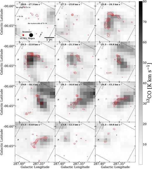
Toward Tr 14, many velocity components overlap along the line of sight. Figure 5 shows a velocity-channel map of the CO integrated-intensity ratio |$R^{12}_{2-1/1-0}$| overlaid on the Spitzer 8 μm emissions toward Tr 14. In the velocity range −30.2 to −20.2 km s−1, CO emissions have been detected only in the region where the intensity of 8 μm emissions are high and the |$R^{12}_{2-1/1-0}$| is higher (∼1.0) at the edges of the clouds, indicating that these molecular clouds are probably interacting with the H ii region of Tr 14. Such characteristics of molecular clouds are observed in other H ii regions as well; e.g., W 51 (Fujita et al. 2019a), which is one of the most active massive-star-forming regions. In the velocity range −20.2 to −12.8 km s−1, |$R^{12}_{2-1/1-0}$| is relatively high (∼0.8) at the edge of the cloud in the western side of Tr 14 (|$l,\, b =\, {\sim}{287{_{.}^{\circ}}37},\, {\sim}{-0{_{.}^{\circ}}65 }$|), although the ratio is low where the CO intensity is low. These results indicate that both the −20 km s−1 cloud and the −14 km s−1 cloud are also interacting with the H ii region of Tr 14, while there may be non-interacting diffuse cloud at the velocity range of −20.2 to −12.8 km s−1. In the velocity range above −12.8 km s−1, |$R^{12}_{2-1/1-0}$| is again high (∼1.0), whereas the CO intensity is relatively low. These emissions may include outflows from young massive stars in Tr 14, as discussed by Yonekura et al. (2005). We need more detailed observations to identify them.
![Velocity channel maps of the integrated-intensity ratio [12CO (J = 2–1)/12CO (J = 1–0)] toward Tr 14. The top left-hand panel and the black contours in the other panels show the Spitzer 8 μm emissions. The 8 μm contours are plotted at every 100 M Jy str−1 from 300 M Jy str−1. The CO integration range for each panel is given in the top left-hand corner of the panel. The CO contours are plotted every 6 K km s−1 from 6 K km s−1. The symbols are the same as in figure 2. The black square in the top left-hand panel indicates the area of the ALMA data shown in figure 7. (Color online)](https://oup.silverchair-cdn.com/oup/backfile/Content_public/Journal/pasj/73/Supplement_1/10.1093_pasj_psaa078/3/m_psaa078fig5.jpeg?Expires=1749109887&Signature=Yk7peG7QTdkNuuntD011iExwRGObuyW1wD9kSeXJegnHUOLLQVbwNg8w2m~AoJxhjsrHQ0Af-0zaNVrd-2tDFI-8Mj9kFM8Vb2HSWps13FysQgH8SGDoLvCcdzxFW-EBQ1yR7H2PHjoD7LmFC2oN8oGthfE0n8S8V998lpkPh72cJJ3WTB3Gd49~mnFjWsv9cad8I2kVz4Fp9hlleTfpfVPBj~gHne~HHRyMHtUiGQuPHTbkCxKmoz-OneKJUqQpgg4Hz5S4hpN2d4KOepWz9NppBI5gd6g1slkk4oCpyba5FCDVBDnH0DM1BX5ZMiZkyHTJOpJGIjrlFZgxZie1gQ__&Key-Pair-Id=APKAIE5G5CRDK6RD3PGA)
Velocity channel maps of the integrated-intensity ratio [12CO (J = 2–1)/12CO (J = 1–0)] toward Tr 14. The top left-hand panel and the black contours in the other panels show the Spitzer 8 μm emissions. The 8 μm contours are plotted at every 100 M Jy str−1 from 300 M Jy str−1. The CO integration range for each panel is given in the top left-hand corner of the panel. The CO contours are plotted every 6 K km s−1 from 6 K km s−1. The symbols are the same as in figure 2. The black square in the top left-hand panel indicates the area of the ALMA data shown in figure 7. (Color online)
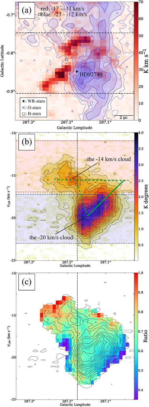
We next investigate the detailed velocity structures of the molecular clouds around Tr 14. Figure 6a shows the 12CO (J = 1–0) integrated-intensity of the −20 km s−1 cloud and the −14 km s−1 cloud toward Tr 14. Figures 6b and 6c show the velocity–galactic latitude (v–b) diagram of the 12CO (J = 1–0) emissions and |$R^{12}_{2-1/1-0}$|, respectively, toward the center of Tr 14. The integration range is indicated by the black dashed lines (range A) in figure 6a. The ratio |$R^{12}_{2-1/1-0}$| is slightly high (∼ 0.7) in the −20 km s−1 cloud and in the higher velocity range of the −14 km s−1 cloud. These results suggest that the two molecular clouds are indeed associated with Tr 14. Figure 6d shows the 12CO (J = 1–0) integrated-intensity in the velocity ranges of −30 to −27 km s−1 and −25 to −22 km s−1. Figures 6e and 6f are the same as figures 6b and 6c, but toward the western side of Tr 14 (range B in figure 6d). The ratio |$R^{12}_{2-1/1-0}$| of the two velocity components is high (∼1.0), suggesting that the two are interacting with the H ii region. We found that the two velocity components exhibit a complementary spatial distribution, which is one of the significant observational signatures of a CCC (e.g., Fukui et al. 2018). The two can be separated in the v–b diagram, indicating that they cannot be explained as a velocity gradient in a molecular cloud. In addition, they show reversed V-shaped structures in figures 6e and 6f. Such V-shaped structures in position–velocity diagrams have been observed in other objects (e.g., Fujita et al. 2019a) as significant observational signatures of a CCC.
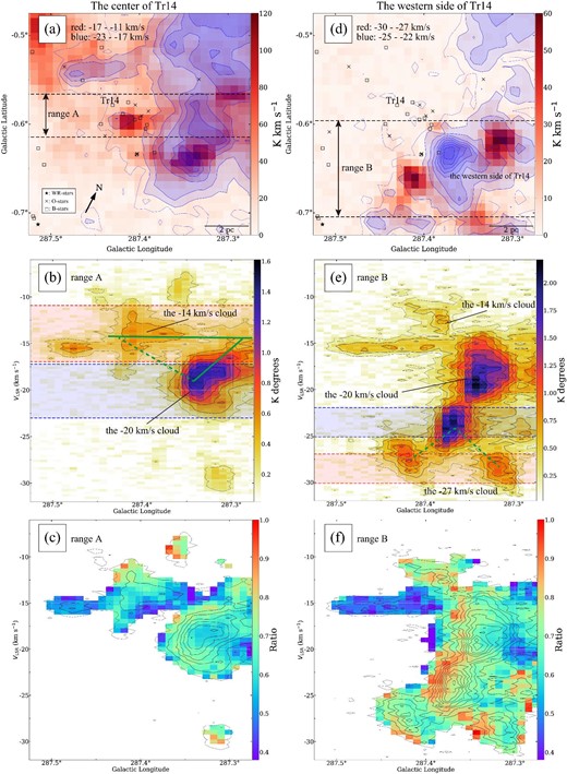
(a) The red image and blue contours show the integrated-intensity of the 12CO (J = 1–0) emissions toward the center of Tr 14. The integrated velocity ranges are shown by the red and blue shading in (b). The contours are plotted at 8, 16, 32, 64, 96, 128, and 160 K km s−1. The symbols are the same as in figure 2. (b) Galactic longitude–velocity (l–v) diagram of the 12CO (J = 1–0) emissions integrated over the range A shown by the dashed lines in panel (a). The contours are plotted every 0.2 K from 0.2 K . (c) Galactic longitude–velocity (l–v) diagram of the intensity ratio 12CO (J = 2–1)/12CO (J = 1–0). (d)–(f) Same as panels (a)–(c), but toward the western side of Tr 14. (Color online)
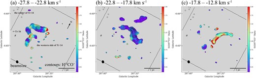
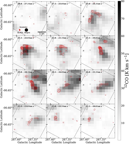
To search for other evidence of a CCC in the western side of Tr 14, we next investigate the shocked gas in this region by using the SiO (v = 0, J = 2–1) and H13CO+ (J = 1–0) emission data obtained with ALMA [2016.1.01609.S (Rebolledo et al. 2020)]. The thermal SiO lines are thought to be a good tracer of hot and shocked gas because the abundance of SiO molecules in a gas phase increases in a high-temperature (Tk > ∼100 K) environment (e.g., Ziurys et al. 1989). Figure 7 shows the velocity channel maps of the integrated-intensity of 12CO (J = 1–0) (gray scale) and SiO (v = 0, J = 2–1) (red contours) toward the western side of Tr 14. The detected SiO emissions are not masers because they have diffused structures in several parsec. In the velocity range −24.3 to −22.8 km s−1, SiO emissions are detected with an arc-like structure at the edge of the molecular cloud traced by the 12CO (J = 1–0) line. These SiO emissions are thought to be tracing photodissociation regions (PDR) induced by the nearby massive stars in Tr 16 and the center Tr 14, as suggested in Rebolledo et al. (2020). On the other hand, H13CO+ (J = 1–0), the rest frequency of which is close to that of SiO (v = 0, J = 2–1), is known as a dense gas tracer, and the ratio SiO/H13CO+ is often used as a shocked molecular gas tracer (e.g., Handa et al. 2006; Amo-Baladrón et al. 2011; Tsuboi et al. 2015; Uehara et al. 2019). Figure 8 shows the integrated-intensity ratio SiO (v = 0, J = 2–1)/H13CO+ (J = 1–0) toward the western side of Tr 14. There is no ratio gradient in the direction of the clusters (Tr 16 and the center of Tr 14), indicating that this ratio is enhanced due to mechanisms other than the radiation from the nearby massive stars. Figure 9a shows the l–v diagram of the 12CO (J = 1–0) (gray scale and gray contours) and SiO (v = 0, J = 2–1) (red contours) integrated from b = −0.68 to b = −0.61. Figure 9b is the same as figure 9a, but only the voxels with a SiO/H13CO+ ratio higher than 2.5 are integrated. This threshold of the ratio is the same value that was used to identify CCCs in Uehara et al. (2019). We can see that the higher ratio gas distributes mainly in three points, (|${287{_{.}^{\circ}}38},\ -25\:$|km s−1), (|${287{_{.}^{\circ}}36},\ -17\:$|km s−1), and (|${287{_{.}^{\circ}}35 },\ -23\:$|km s−1). In the l–v diagram, the gas in (|${287{_{.}^{\circ}}38},\ -25\:$|km s−1) is located between the two clouds, the velocity ranges of which are −30 to −27 km s−1 and −25 to −22 km s−1, respectively. The ratio enhancement of this region can be interpreted as being due to the shock induced by the CCC between the cloud at −25 to −22 km s−1 and the −27 km s−1 cloud, which strongly supports the CCC scenario proposed above. Similarly, the high ratio gas in (|${287{_{.}^{\circ}}36 },\ -17\:$|km s−1) suggests a collision between the −20 km s−1 cloud and the −14 km s−1 cloud. The high ratio gas in (|${287{_{.}^{\circ}}35},\ -23\:$|km s−1) is detected between the cloud at −25 to −22 km s−1 and the −20 km s−1 cloud. This result may indicate a collision between them, but we cannot conclude as such at this time. For these reasons, we propose a CCC scenario involving these four clouds as the triggering mechanism for the formation of the massive stars in the western side of Tr 14.
Velocity channel maps of the integrated-intensity of 12CO (J = 1–0) (gray scale) and SiO (v = 0, J = 2–1) (red contours) obtained with ALMA toward the western side of Tr 14. The symbols are the same as in figure 2. The contours are plotted every 0.12 Jy beam−1 km s−1 from 0.12 K km s−1. The black lines indicate the area of the ALMA data. (Color online)
Integrated-intensity ratio SiO (v = 0, J = 2–1)/H13CO+ (J = 1–0) toward the western side of Tr 14. The contours show the integrated-intensity of H13CO+ (J = 1–0). The contours are plotted every 0.2 Jy beam−1 km s−1 from 0.1 Jy beam−1 km s−1. (Color online)
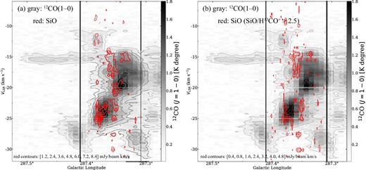
(a) Galactic longitude–velocity (l–v) diagram of the 12CO (J = 1–0) (gray scale and gray contours) and SiO (v = 0, J = 2–1) (red contours) integrated from b = −0.68 to b = −0.61. The gray contours are plotted every 0.2 K from 0.2 K . The red contours are plotted every 1.2 mJy beam−1 degree (∼ 5σ) from 1.2 mJy beam−1 degree. The black vertical dashed lines indicate the area of the ALMA data. (b) Same as panel (a), but only the voxels with SiO/H13CO+ ratios of higher than 2.5 are integrated. The red contours are plotted every 1.2 mJy beam−1 degree from 0.6 mJy beam−1 degree. (Color online)
4.1.2 Tr 15
Figure 10a shows the 12CO (J = 1–0) integrated-intensity of the −20 km s−1 cloud and the −14 km s−1 cloud toward Tr 15. One O-star and several B-stars are located at |$(l,\, b)=({287{_{.}^{\circ}}44},\ -{0{_{.}^{\circ}}40})$|, where there is both an intensity valley in the −14 km s−1 cloud and the edge of the −20 km s−1 cloud. For figures 4b2 and 4c2, the ratios |$R^{12}_{2-1/1-0}$| are high (∼0.8) in both the −20 km s−1 cloud and the −14 km s−1 cloud near Tr 15, indicating that these two are interacting with the H ii region of Tr 15. The −8 km s−1 cloud is also detected in this region, but it is probably not interacting with the H ii region because of its low |$R^{12}_{2-1/1-0}$| (∼0.4). Figures 10b and 10c show the v–b diagram of the 12CO (J = 1–0) emissions and |$R^{12}_{2-1/1-0}$|, respectively, toward Tr 15. We found that the v–b diagram shows a V-shaped structure. This characteristic in the position–velocity diagram resembles those in the numerical simulation of a CCC by Takahira, Tasker, and Habe (2014) and Haworth et al. (2015). In this simulation, two molecular clouds of different sizes (one twice as large as the other) collide at a relative velocity of 5 km s−1 (see table 3 in Fukui et al. 2018). Figure 10 shows the position–velocity (p–v) diagram of an artificial observation of this simulation at the viewing angle of 45°. Owing to this viewing angle, the p–v diagram shows an asymmetric feature. Similarly to the western side of Tr 14, a CCC between the two clouds may have taken place, triggering massive-star formation in Tr 15.


(a)–(c) Same as figure 6, but toward Tr 15. (d) Position–velocity diagram of the simulation by Takahira, Tasker, and Habe (2014) and Haworth et al. (2015), and used in Fukui et al. 2018. The epoch is 1.6 Myr after the onset of the collision and the viewing angle is 45°, respectively (see figure 4 in Fukui et al. 2018). The integration range is from −2.5 to +2.5 pc along an axis perpendicular to the collision axis. (Color online)
4.1.3 Tr 16
In figures 1a and 1b, the Southern Cloud is clearly interacting with the H ii regions formed by the massive stars in Tr 16 , because the cloud traced by CO corresponds to the distribution of 8 μm emissions. The Southern Cloud has a velocity gradient of ∼5 km s−1 over the whole area (figure 3a). The H ii region is already extended by a few tens of parsecs, and weak emissions are detected from the −20 km s−1 and the −14 km s−1 cloud at the center of Tr 16. In order to investigate the molecular clouds associated with Tr-16, it will be necessary to observe them with both deep sensitivity and high spatial resolution.
4.1.4 HD 92740
HD 92740 is an isolated WR-star located west of Tr 14. Figure 11a shows the 12CO (J = 1–0) integrated-intensity of the −20 km s−1 cloud and the −14 km s−1 cloud toward HD 92740. We found that the two clouds exhibit a complementary distribution also in this region. HD 92740 is located at the interface between them. Figures 11b and 11c show the l–v diagram of the 12CO (J = 1–0) emissions and the l–v diagram of |$R^{12}_{2-1/1-0}$|, respectively, toward HD 92740. In the l–v diagrams, the two clouds are separated into discrete clouds, rather than appearing to be one molecular cloud with a velocity gradient. For these reasons, it is possible that a CCC between the two clouds took place and triggered the formation of HD 92740 similarly to the western side of Tr 14 and Tr 15.
(a)–(c) Same as figure 6, but toward HD 92740. The contours in panels (b) and (c) are plotted every 0.3 K from 0.3 K . The vertical dashed line in panels (b) and (c) indicates the position of HD 92740. (Color online)
4.2 Cloud–cloud collision scenario in the CNC
As discussed above, we found the signatures of a CCC in three regions: the western side of Tr 14, near Tr 15, and near HD 92740. The radial velocities of the pair of colliding clouds in Tr 15 and HD 92740, the −20 km s−1 cloud and the −14 km s−1 cloud, are the same, and their p–v diagrams are similar to each other. Figure 12a shows the 12CO (J = 1–0) integrated-intensity distributions of the −20 km s−1 cloud (contours) and the −14 km s−1 cloud (image). The two clouds show complementary distributions through the entire region of the Northern Cloud, implying that they are colliding over a 10-pc scale. If so, the −14 km s−1 cloud may have a cavity of the same size and shape as the −20 km s−1 clouds. This cavity would have been formed at the onset of the collision.
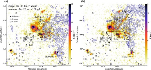
(a) The color image and blue contours show the integrated-intensity of the 12CO (J = 1–0) emissions toward the CNC integrated over −13.8 to −13.3 km s−1 and −20.9 to −20.4 km s−1, respectively. The contours are plotted every 2.2 K km s−1 (5σ) from 2.2 K km s−1. The symbols are the same as in figure 2. (b) The same as panel (a), but with the blue contours (the −20 km s−1 cloud) displaced along the black arrows. (Color online)
To search for such a cavity, we first quantify the complementarity between the two molecular clouds. We adopted Spearman’s rank correlation coefficient between the integrated-intensity distributions of the two clouds as the index of complementarity. If the two show a complementary distribution, the correlation coefficient between them is negative; that is, the lower correlation coefficient (anti-correlation) indicates that the complementarity is high. To calculate the coefficients, we determined the area of the −20 km s−1 cloud (the contours in figure 12a) as shown by the black rectangle in figure 12a. We then define area of the same size for the −14 km s−1 cloud (the image in figure 12a) as a function of the x-axis (galactic longitude) displacement and y-axis (galactic latitude) displacement, and we calculated the coefficients between the two intensity distributions. In the calculating of the correlation coefficients, we removed those pixels with values of <10σ for both clouds. Figure 13 shows the calculated correlation coefficients for each direction of displacement (see appendix 1). The black square at (0, 0) indicates the original position (without displacements) of the two integrated-intensity distributions shown in figure 12a. We found that the two distributions shows a minimum correlation coefficient (∼−0.75) for a displacement of (x-axis displacement, y-axis displacement) = (−3.0 pc, 5.3 pc) ≈ 6 pc, indicated by the arrows in figure 12b. Figure 12b shows the integrated-intensity distributions of the −14 km s−1 cloud and the −20 km s−1 cloud displaced by this value. This may be the most complementary distribution of the two clouds, indicating that the collision between them started at this relative position where Tr 15 is located. Accordingly, the massive stars in Tr 15 may have formed early in the collision.
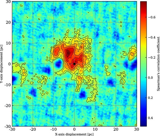
Distribution of Spearman’s correlation coefficient as a function of displacements in the x-axis (galactic longitude) direction and in the y-axis (galactic latitude) direction. The contour levels are −0.74, −0.70, −0.60, −0.50, −0.40, −0.30, and −0.20. (Color online)
Next, we estimate the timescale of the collision by using the position of the cavity calculated above. The calculated displacement of 6 pc corresponds to the cavity length on the plane of the sky. Because we cannot measure the velocity difference between the two clouds along the cavity, we tentatively assume that it is the same as the velocity separation along the line-of-sight, 6 km s−1. Thus, we estimate the timescale of the collision to be roughly 6 [pc]/(6 [km s−1]) = ∼1 × 10⁶ [yr]. This estimated collision timescale is consistent with the ages of the clusters [2–3 Myr for Tr 14 (Preibisch et al. 2011) and 6 ± 3 Myr for Tr 15 (Feinstein et al. 1980; Morrell et al. 1988; Smith 2006b)] within a factor of 2–3, although both of these estimates are rough.
In sub-subsection 4.1.1, we found evidence for a CCC between the molecular clouds with the velocities of ∼−27 km s−1 and ∼−23 km s−1 in the western side of Tr 14. The two clouds are now in a complementary distribution and the number of identified massive stars is small, so probably only a small amount of time has passed since the collision started. On the other hand, in the center of Tr 14, the p–v diagram of the clouds (figure 6b) can be interpreted as a CCC between the −20 km s−1 cloud and the −14 km s−1 cloud as indicated by the green V-shape, as for Tr 15. Therefore, the massive stars triggered by these two CCCs may have overlapped along the line of sight or have been mixed into Tr 14. Clarifying this situation will require more detailed observations with higher angular resolution. Figure 14 shows a sketch diagram of this collision scenario between the −20 km s−1 cloud and the −14 km s−1 cloud in the Northern Cloud.
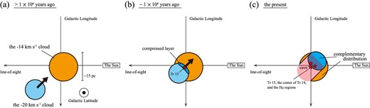
Sketch diagram of the Northern Cloud as viewed from the Galactic north pole. (a) Before the collision started (> 1 × 10⁶ yr ago). Blue and orange represent the −20 km s−1 cloud and the −14 km s−1 cloud, respectively. (b) The epoch when the collision has started and a little time has elapsed (∼ 1 × 10⁶ yr ago). The deep blue region indicates the compressed layer between the two clouds, where star(s) form. (c) The present. The two clouds show the complementary distributions for observers in the solar system. (Color online)
In the region near HD 92740, only the one WR-star, HD 92740, formed. It is probable that the lack of massive stars in this region may be due to the lower mass of one of the colliding clouds (figure 11a). Only a few molecular clouds have been associated with the region around Tr 16, perhaps because of strong feedback from the massive stars including η-Carinae. It is uncertain whether the formation of the massive stars in Tr 16 is related to the CCC we have suggested.
5 Summary
The main conclusions of the present study are summarized as follows:
We presented analyses of the velocity structures of the molecular clouds in the CNC by using the 12CO and 13CO (J = 1–0) archival datasets obtained with the Mopra telescope and the 12CO (J = 2–1) dataset obtained with NANTEN2.
We found that the molecular clouds in the CNC can be separated into four clouds at the velocities −27, −20, −14, and −8 km s−1. Their masses are 0.7 × 10⁴ M⊙, 5.0 × 10⁴ M⊙, 1.6 × 10⁴ M⊙, and 0.7 × 10⁴ M⊙, respectively. Most of them are likely associated with the clusters because of the high 12CO (J = 2–1)/12CO (J = 1–0) intensity ratio and the correspondence with the Spitzer 8 μm distributions.
We found the observational signatures of cloud–cloud collisions in near Tr 14, Tr 15, and HD 92740; namely, a V-shaped structure and a complementary spatial distribution, between the −20 km s−1 cloud and the −14 km s−1 cloud. Furthermore, we found that SiO emission, which is a tracer of a shocked molecular gas, is enhanced between the colliding clouds by using ALMA archive data.
We propose a scenario wherein the formation of massive stars in the clusters and the formation of HD 92740 were triggered by a collision between the two clouds. The timescale of the collision is estimated to be ∼1 Myr, which is roughly comparable to the ages of the clusters estimated in previous studies.
Acknowledgements
This study was financially supported by Grants-in-Aid for Scientific Research (KAKENHI) of the Japanese society for the Promotion of Science (JSPS; grant numbers 15H05694, 15K17607, 17H06740, and 18K13580) and the ALMA Japan Research Grant of NAOJ ALMA Project (NAOJ-ALMA-245). The authors would like to thank the all members of the Mopra, NANTEN2 and ALMA (project code: 2016.1.01609.S) for providing the data. Data analysis was carried out by using Astropy (Astropy Collaboration 2013), APLpy (Robitaille & Bressert 2012). The authors also would like to thank NASA for providing FITS data of the WISE and the Spitzer Space Telescope.
Appendix 1. H13CO+ emission in the western side of Tr 14
Figure 15 shows the velocity channel maps of the integrated-intensity of 12CO (J = 1–0) (gray scale) obtained with Mopra and H13CO+ (J = 1–0) (red contours) obtained with ALMA toward the western side of Tr 14.
Velocity channel maps of the integrated-intensity of 12CO (J = 1–0) (gray scale) and H13CO+ (J = 1–0) (red contours) obtained with ALMA toward the western side of Tr 14. The symbols are the same as in figure 2. The contours are plotted every 0.24 Jy beam−1 km s−1 from 0.12 K km s−1. The black lines indicate the area of the ALMA data. (Color online)
Appendix 2. Complementarity calculation using Spearman’s rank correlation coefficient
We first defined the area of the −20 km s−1 cloud as shown by the black rectangle in figure 16a. Next, we calculated rS between the integrated intensities of the −14 km s−1 cloud (the image) and the −20 km s−1 cloud (the blue contours) pixel-to-pixel within the given area. Figure 17a shows scatter plots of the integrated intensities of the two clouds. The left- and right-hand panels show the raw integrated intensities and the rankings, respectively. In this calculation, we removed pixels for which the values are both <10σ. As a result, we calculate rS − 0.67 at the original position A.

Same as figure 12a. (a) The blue contours (−20 km s−1 cloud) are displaced by (x-axis displacement, y-axis displacement) = (0 pc, 0 pc). (b) The blue contours are displaced by (−3.0 pc, 5.3 pc). (c) The blue contours are displaced by (−7.7 pc, −0.3 pc). (Color online)
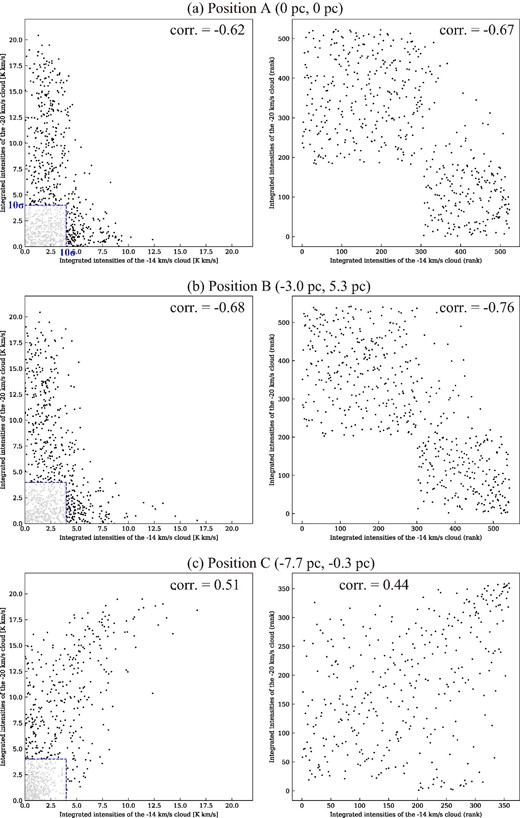
Scatter plot of the integrated intensities of the −14 km s−1 cloud (x-axis) and the −20 km s−1 cloud (y-axis). The left- and right-hand panels show the raw integrated intensities and the rankings, respectively. (Color online)
Similarly, we calculate rS for each displacement (x-axis displacement, y-axis displacement) by a unit of one pixel. In the present study, one pixel corresponds to 0.33 pc. Figure 18 shows a map of the calculated values of rS. The minimum occurs at the displacement (x-axis displacement, y-axis displacement) = (−3.0 pc, 5.3 pc) (position B in figure 18). There the two clouds show the most complementary distribution (figure 16b). In contrast, at the local maximum the displacement is (x-axis displacement, y-axis displacement) = (−7.7 pc, −0.3 pc) (position C in figure 18), and the two clouds show similar distributions (figure 16c).
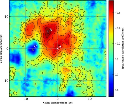
Distribution of Spearman’s correlation coefficient rS as a function of displacements along the x-axis (galactic longitude) direction and along the y-axis (galactic latitude) direction. The contour levels are −0.74, −0.70, −0.60, −0.50, −0.40, −0.30, and −0.20. The white crosses labeled A, B, and C correspond to the displacements shown in figure 16. (Color online)
