


Abstract
The Rossiter–McLaughlin (RM) effect has been widely used to estimate the sky-projected spin-orbit angle, λ, of transiting planetary systems. Most of the previous analysis assumes that the host stars are rigid rotators in which the amplitude of the RM velocity anomaly is proportional to v⋆ sin i⋆. When their latitudinal differential rotation is taken into account, one can break the degeneracy, and determine separately the equatorial rotation velocity v⋆ and the inclination i⋆ of the host star. We derive a fully analytic approximate formula for the RM effect adopting a parametrized model for the stellar differential rotation. For those stars that exhibit a differential rotation similar to that of the Sun, the corresponding RM velocity modulation amounts to several m s−1. We conclude that the latitudinal differential rotation offers a method to estimate i⋆, and thus the full spin-orbit angle ψ, from the RM data analysis alone.
1 Introduction
For isolated and stable systems like our solar system, ψ is supposed to keep the initial value at the formation epoch. For instance, in the simplest scenario, the star and the surrounding protoplanetary disk are likely to share the same direction of the angular momentum of the progenitor molecular cloud (Takaishi et al. 2020). Therefore planets formed in the disk are expected to have ψ ∼ 0, as is the case for all the eight solar planets (ψ < 6°).
Such a naive expectation, however, is not necessarily the case for the observed distribution of λ (Xue et al. 2014; Winn & Fabrycky 2015); more than
We would like to stress that spin-orbit misaligned systems are often defined by the values of λ alone that are measured from the Rossiter–McLaughlin (RM) effect, which is the radial velocity anomaly of the host star due to a distortion of the stellar line profiles during the planetary transit (e.g., Rossiter 1924; McLaughlin 1924; Ohta et al. 2005; Winn et al. 2005).
While λ has been measured for more than 150 transiting systems,1 i⋆ values are available from asteroseismology for only a couple of systems, Kepler-25c and HAT-P-7 (Benomar et al. 2014), and about 30 systems have i⋆ estimated spectroscopically from equation (3); see Hirano et al. (2012), for example. More recently, Louden et al. (2021) derived a statistical distribution of 〈sin i⋆〉 for a sample of 150 Kepler stars with transiting planets smaller than Neptune. Therefore, a complementary method to estimate i⋆ breaking the degeneracy in v⋆sin i⋆ is essential to understand the distribution of the spin-orbit angle ψ (cf. Albrecht et al. 2021).
The RM effect of transiting planets was measured by Queloz et al. (2000) for the first time. Ohta et al. (2005) derived an analytic approximate formula for the RM effect, which was improved later by Hirano et al. (2010, 2011b). Such analytic expressions for the RM effect are useful in understanding the parameter dependence and degeneracy that are not easy to extract from numerical analysis. Furthermore, Hirano et al. (2011a, 2011b) attempted to examine the effect of the differential rotation for the rapidly rotating XO-3 system (v⋆ sin i⋆ ≈ 18 m s−1 and λ ≈ 40°), but their result was not so constraining, mainly due to the large stellar jitter for such host stars (∼15 m s−1).
In the present paper, we improve the previous model for the RM effect incorporating the differential rotation of the host star. Since our model is fully analytic, one can clearly understand how i⋆ and λ can be inferred from the RM modulation due to the differential rotation; see equation (30) below. We find that the differential rotation similar to the Sun produces an additional feature of an amplitude of the order of several m s−1 in the RM effect, which should be detectable for systems with good signal-to-noise ratios. Thus our analytic formula is useful in breaking the degeneracy of v⋆sin i⋆, and allows the determination of i⋆, and thus the true spin-orbit angle ψ, for transiting planetary systems with the differential rotation of the host stars.
2 Coordinates of the star and the transiting planet in the observer’s frame
We introduce three coordinate systems for the present analysis, the origin of which is chosen as the center of the host star. The observer’s frame (O-frame) is represented by (X, Y, Z). The Z-axis is directed toward the observer, and the Y-axis is chosen in such a way that the orbital angular momentum vector of the planet lies on the YZ plane (figure 1).
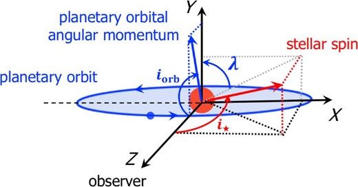
Spin-orbit architecture of transiting planetary systems in the observer’s frame (O-frame); i⋆ and iorb are the stellar inclination and the planetary orbital inclination with respect to the observer, while λ is the sky-projected spin-orbit angle. (Color online)
The planetary frame (P-frame) is represented by
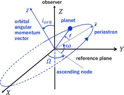
Planetary orbit in the observer’s frame (X, Y, Z) and in the planetary frame
3 Radial component of the stellar surface rotation velocity at the projected position of the transiting planet
4 Differential rotation effect for a circular planetary orbit
5 Analytic approximation to the Rossiter–McLaughlin effect for differentially rotating stars
5.1 The Rossiter–McLaughlin effect in Gaussian approximation
The stellar lines are additionally broadened by the stellar rotation, the Gaussian width of which is found to be approximated as equation (35) by Hirano et al. (2010). Note that Hirano et al. (2010, 2011b) adopted the Gaussian profile
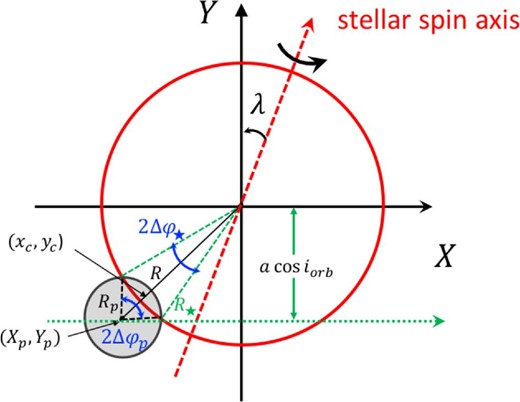
Schematic illustration of the stellar disk occulted by a transiting planet at the ingress/egress phases. (Color online)
5.2 Effect of limb darkening
6 Results
Equation (32) with equations (45) and (46) provides an analytic formula for the RM velocity anomaly taking account of the differential rotation of the host star.
| Name | Symbol | Fiducial value | Reference |
|---|---|---|---|
| Star | |||
| Radius | R⋆ | Casasayas-Barris et al. (2021) | |
| Spin velocity | v⋆ sin i⋆ | 4.5 km s−1 | Hirano et al. (2011b) |
| Gaussian fitting | β | 4.0 km s−1 | Hirano et al. (2011b) |
| ζ | 4.3 km s−1 | Hirano et al. (2011b) | |
| σ⋆ | Hirano et al. (2011b) | ||
| Limb darkening | (q1, q2) | (0.56, 0.32) | Hirano et al. (2010) |
| Differential rotation | (α2, α4) | (0.163, 0.121) | Snodgrass and Ulrich (1990) Solar value |
| Planet | |||
| Radius ratio | Rp/R⋆ | 0.121 | Casasayas-Barris et al. (2021) |
| Orbit | |||
| Orbital period | Porb | 3.5 d | Casasayas-Barris et al. (2021) |
| Semi-major axis | a | 0.047 au | Casasayas-Barris et al. (2021) |
We adopt fiducial values of parameters mainly from the HD 209458 system except for iorb, i⋆, λ, and the differential rotation parameters (α2, α4). For simplicity, we consider a circular orbit (e = 0), and thus fix ω = 0 and Ω = π without loss of generality.
| Name | Symbol | Fiducial value | Reference |
|---|---|---|---|
| Star | |||
| Radius | R⋆ | Casasayas-Barris et al. (2021) | |
| Spin velocity | v⋆ sin i⋆ | 4.5 km s−1 | Hirano et al. (2011b) |
| Gaussian fitting | β | 4.0 km s−1 | Hirano et al. (2011b) |
| ζ | 4.3 km s−1 | Hirano et al. (2011b) | |
| σ⋆ | Hirano et al. (2011b) | ||
| Limb darkening | (q1, q2) | (0.56, 0.32) | Hirano et al. (2010) |
| Differential rotation | (α2, α4) | (0.163, 0.121) | Snodgrass and Ulrich (1990) Solar value |
| Planet | |||
| Radius ratio | Rp/R⋆ | 0.121 | Casasayas-Barris et al. (2021) |
| Orbit | |||
| Orbital period | Porb | 3.5 d | Casasayas-Barris et al. (2021) |
| Semi-major axis | a | 0.047 au | Casasayas-Barris et al. (2021) |
We adopt fiducial values of parameters mainly from the HD 209458 system except for iorb, i⋆, λ, and the differential rotation parameters (α2, α4). For simplicity, we consider a circular orbit (e = 0), and thus fix ω = 0 and Ω = π without loss of generality.
6.1 Dependence on the differential rotation parameters
Figure 4 illustrates schematic trajectories of planets during their transits for different combinations of the spin-orbit angles (i⋆, λ). The corresponding RM velocity anomaly ΔvRM for each panel is plotted in figures 5 and 6 for iorb = 90°(b = 0) and 87°(b ≈ 0.47), respectively, for different combinations of α2 and α4.
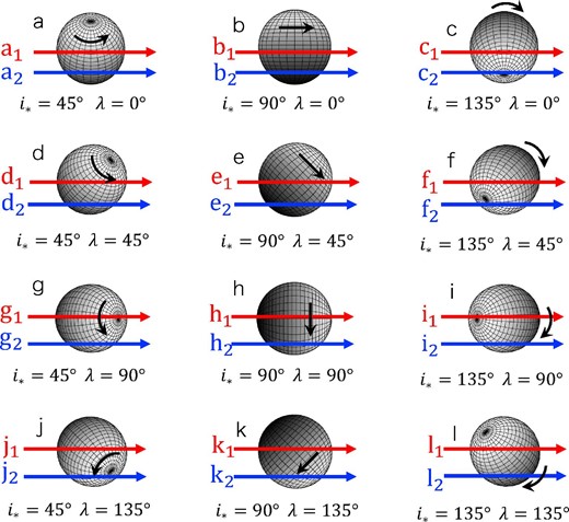
Schematic trajectories of transiting planets on the stellar disk for different i⋆ and λ. Upper and lower arrows in each panel illustrate trajectories for iorb = 90°(b = 0) and
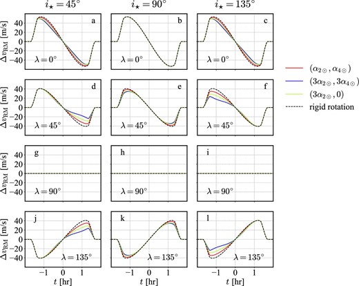
Effect of the stellar latitudinal differential rotation on the RM velocity anomaly ΔvRM(t) for iorb = 90°(b = 0) for different values of λ and i⋆. Each panel corresponds to the upper trajectories shown in figure 4. Red, blue, and green curves are for (α2, α4) = (α2⊙, α4⊙), (3α2⊙, 3α4⊙), and (3α2⊙, 0), respectively. Dashed curves indicate the case for rigid rotation (α2 = α4 = 0). We do not plot the case for (α2, α4) = (0, 3α4⊙) because it is very close to models with (α2, α4) = (α2⊙, α4⊙). (Color online)
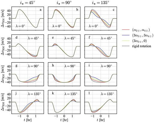
Same as figure 5 except for iorb = 87°(b ≈ 0.47). (Color online)
First, let us consider panels a to c in figure 5, in which iorb = 90° and λ = 0. Since planets in panels a and c move away from the stellar equator (figure 4), the corresponding ΔvRM(t) with differential rotation becomes smaller than that for rigid rotator. Due to the symmetry between l ↔ − l in equation (16), ΔvRM(t) in panels a and c is identical. In contrast, panel b corresponds to the planetary trajectory along the equator (figure 4), and ΔvRM(t) is not affected by the presence of differential rotation.
Similarly, one may understand the behavior of panels d to f (λ = 45°) by comparing with the corresponding trajectories in figure 4. Since the trajectory d1 moves from low to high latitude regions, the effect of differential rotation is stronger after the central transit epoch as shown in figure 5. The trajectory f1 is the opposite, and the trajectory e1 corresponds to the case between the two cases.
Panels j to l (λ = 135°) are easily understood from panels d to f since equations (18) and (19) indicate Vz(λ) = −Vz(π − λ) for iorb = 90°. Finally, panels g to i (λ = 90°) correspond to the trajectories with Vz = 0 for iorb = 90°.
Consider next the case for iorb = 87°(b ≈ 0.47), i.e., figure 6 and lower trajectories in the corresponding panels of figure 4. In this case, the symmetry between λ ↔ π − λ no longer holds, and ΔvRM(t) exhibits small but clear dependence on iorb, i⋆, and λ.
In conclusion, figures 5 and 6 imply that the differential rotation can be used to estimate i⋆ from the RM velocity anomaly curve through the latitudinal dependence of
6.2 Sensitivity to the stellar inclination
Figure 7 compares ΔvRM with and without differential rotation for different values of (iorb, λ). Figure 8 plots the corresponding RM modulation term due to the differential rotation alone, ΔvRM(i⋆) − ΔvRM(rigid rotation). In most cases, the amplitude of the modulation term becomes largest around the ingress/egress phases, while it is suppressed by the limb darkening depending on the specific values of iorb and λ. The modulation term vanishes at the central transit epoch if iorb = 90° and/or λ = 0 because Vdiff(0)∝cos iorbsin λ, as is understood from equation (29).
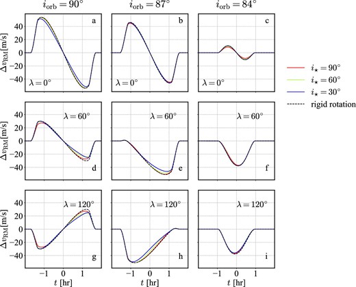
Dependence of ΔvRM on the stellar inclination i⋆, where the equatorial velocity v⋆ sin i⋆ is fixed (4.5 km s−1). Dashed lines correspond to the rigid rotation model. Left-hand, middle, and right-hand panels correspond to iorb = 90°(b = 0), 87°(b ≈ 0.47), and 84°(b ≈ 0.93). Red, green, and blue curves indicate i⋆ = 90°, 60°, and 30°, respectively, for the differential rotation model with α2 = α2⊙ and α4 = α4⊙. (Color online)
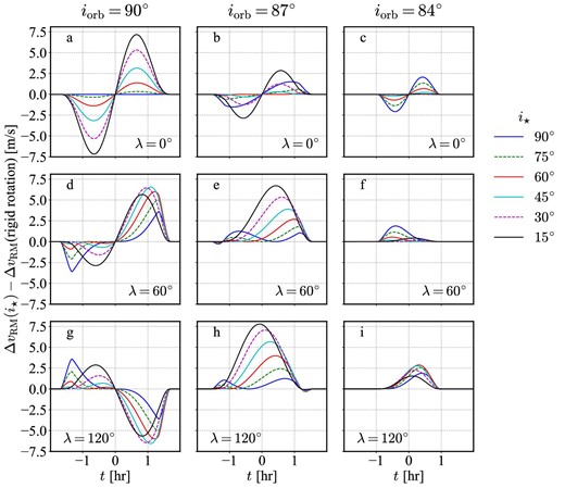
RM modulation term due to the differential rotation after subtracting the rigid rotation component. Each panel adopts the values of λ and iorb in the corresponding panel of figure 7. We adopt α2 = α2⊙ and α4 = α4⊙. Blue solid, green dashed, red solid, cyan solid, purple dashed, and black solid curves correspond to i⋆ = 90°, 75°, 60°, 45°, 30°, and 15°, respectively. (Color online)
Figure 9 plots the maximum values of the RM modulation term during the entire transit period as a function of i⋆. If the degree of the differential rotation for the Sun is assumed, the RM effect is supposed to have an additional modulation component of an amplitude of several m s−1 relative to the rigid rotation case. Given the current precision of the high-resolution radial velocity measurement, it should be detectable for systems with relatively high signal-to-noise ratios.
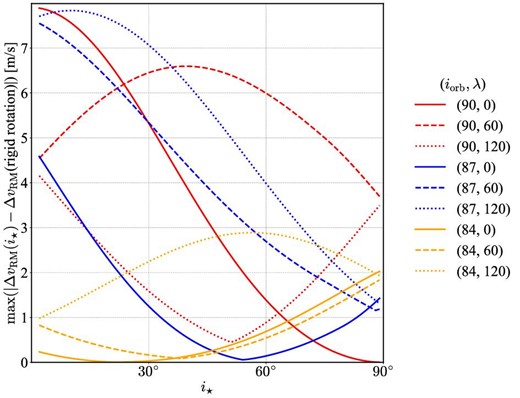
Maximum value of the RM modulation term due to the differential rotation during the entire transit period as a function of i⋆ for different values of iorb and λ indicated in the legend. We adopt α2 = α2⊙ and α4 = α4⊙. Red, blue, and orange curves assume iorb = 90°(b = 0), 87°(b ≈ 0.47), and 84°(b ≈ 0.93), while solid, dashed, and dotted lines correspond to λ = 0°, 60°, and 120°, respectively. (Color online)
6.3 Uncertainties of the spectroscopic parameters
We have shown that, once the stellar differential rotation effect is taken into account, the precise measurement of the RM velocity anomaly ΔvRM can estimate both the stellar inclination i⋆ and the projected spin-orbit angle λ. So far, however, we assumed that the parameters β and ζ in equations (34) and (33) are precisely determined from the stellar spectroscopy. In reality, however, the accurate determination of the two parameters is not so easy (e.g., Kamiaka et al. 2018).
Thus it may be possible that the uncertainties of β and ζ are degenerate with the stellar differential rotation effect. Since a comprehensive study of the parameter degeneracy is beyond the scope of this paper, we decided to show several examples. Figure 10 plots the dependence on β and ζ; strictly speaking, equations (32), (33), and (34) indicate that ΔvRM depends on the combination of β2 + ζ2 under the Gaussian approximation that we adopted throughout the paper. Comparison with figure 6 implies that while the uncertainties of the spectroscopic parameters distort the RM velocity anomaly curve, the distortion pattern is rather different from the signature due to the differential rotation.
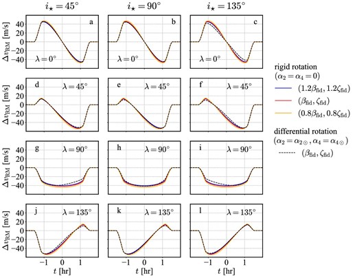
Same as figure 6 (iorb = 87°), but for different sets of the values of β and ζ characterizing the spectroscopic line profiles. Solid lines correspond to the rigid rotation model (α2 = α4 = 0); blue, red, and orange curves correspond to (β, ζ) = (1.2βfid, 1.2ζfid), (βfid, ζfid), and (0.8βfid, 0.8ζfid), respectively. For reference, the fiducial differential rotation model (α2 = α2⊙, α4 = α4⊙, β = βfid, and ζ = ζfid) is plotted in dashed curves. The fiducial values of the parameters are summarized in table 1. (Color online)
For a more quantitative comparison, we plot in figure 11 the residual of ΔvRM(α2, α4, β, ζ) relative to that for the rigid rotation with fiducial spectroscopic parameters, i.e., ΔvRM(α2 = α4 = 0, βfid, ζfid). The resulting distortion due to the inaccuracy of the spectroscopic parameter is sensitive to the value of λ, but independent of the value of i⋆, while the signature of the differential rotation model is sensitive to both λ and i⋆. Figure 11 implies that if the RM velocity anomaly is determined with a precision of the order of m s−1, one can identify the differential rotation signal even under the presence of a relatively large uncertainty of β and ζ.
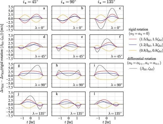
RM velocity anomaly ΔvRM(α2, α4, β, ζ) relative to that for the rigid rotation with fiducial spectroscopic parameters, ΔvRM(α2 = α4 = 0, βfid, ζfid). Solid lines correspond to the rigid rotation model (α2 = α4 = 0); red, blue, and orange curves correspond to (β, ζ) = (1.5βfid, 1.5ζfid), (1.2βfid, 1.2ζfid), and (0.8βfid, 0.8ζfid), respectively. For reference, the fiducial differential rotation model (α2 = α2⊙, α4 = α4⊙, β = βfid, and ζ = ζfid) is plotted in dashed curves. (Color online)
7 Summary and conclusions
The RM effect has unveiled an unexpected diversity of spin-orbit architecture of transiting planetary systems. Most of the previous approaches have assumed a rigid rotation of the host star, and thus were not able to estimate the stellar inclination i⋆ except for the combination of v⋆sin i⋆. We have improved the previous model of the RM effect by incorporating the differential rotation of the host star. Since our model is fully analytic, it provides a good theoretical understanding of how one can determine λ and i⋆ simultaneously from the differential rotation effect.
The latitudinal differential rotation of planetary host stars leaves an additional characteristic signature on the RM effect through equation (28). More specifically, under the Gaussian approximation of stellar lines, the RM effect is analytically described by equation (32), together with equations (33), (34), (45), and (46). We can estimate the values of the spectroscopic parameters, βp and β⋆, and the limb darkening parameters, q1 and q2, from photometric and spectroscopic observations of the host star. If the differential rotation of the star is absent, equation (28) vanishes, and equation (27) is specified by v⋆ sin i⋆ and λ. This provides a widely used method to estimate the projected spin-orbit angle λ from the RM effect. The differential rotation term, equation (28), makes it possible to estimate α2, α4, and i⋆ separately.
The amplitude of the RM modulation term due to the differential rotation is on the order of several m s−1 for stars similar to the Sun, and thus should be detectable for systems with reasonably high signal-to-noise ratio of the RM measurement. Therefore, our model is useful in recovering the full spin-orbit angle ψ (equation 1) based on the RM data analysis alone, in principle. In reality, the degeneracy among several parameters might complicate the interpretation of the differential rotation feature in a robust fashion. A preliminary result shown in figure 11 implies, however, that the uncertainties due to the spectroscopic line profiles are distinguishable from the real differential rotation signature, depending on the values of i⋆ and λ of specific systems. We plan to perform a further study of the parameter degeneracy, and to apply the current methodology to a sample of transiting planetary systems, which will be discussed elsewhere.
Acknowledgments
We thank an anonymous referee and Teruyuki Hirano for many useful and constructive comments. The present work is supported by Grants-in Aid for Scientific Research by the Japan Society for Promotion of Science (JSPS) No.18H012 and No.19H01947, and from JSPS Core-to-core Program “International Network of Planetary Sciences”.
