


Abstract
We have conducted mapping observations toward the n3 and n5 positions in the NGC 2264-D cluster-forming region with the Atacama Compact Array (ACA) of the Atacama Large Millimeter/submillimeter Array (ALMA) in Band 3. Observations with a 10000 au scale beam reveal the chemical composition at the clump scale. The spatial distributions of the observed low upper-state-energy lines of CH3OH are similar to those of CS and SO, and the HC3N emission seems to be predominantly associated with clumps containing young stellar objects. The turbulent gas induced by the star formation activities produces large-scale shock regions in NGC 2264-D, which are traced by the CH3OH, CS, and SO emissions. We derive the HC3N, CH3CN, and CH3CHO abundances with respect to CH3OH. Compared to the n5 field, the n3 field is farther (in projected apparent distance) from the neighboring NGC 2264-C, yet the chemical composition in the n3 field tends to be similar to that of the protostellar candidate CMM3 in NGC 2264-C. The HC3N|$/$|CH3OH ratios in the n3 field are higher than those in the n5 field. We find an anti-correlation between the HC3N|$/$|CH3OH ratio and their excitation temperatures. The low HC3N|$/$|CH3OH abundance ratio at the n5 field implies that the n5 field is an environment with more active star formation compared with the n3 field.
1 Introduction
Clusters are major sites of star formation, and almost |$90\%$| of stars are born in clusters (Lada & Lada 2003). Hence, it is important to study physical conditions and evolution of clusters for the understanding of star formation. Furthermore, clusters are essential from the point of view of the formation of the solar system, because several studies suggest that the Sun was born in a cluster region (Adams 2010). Jensen et al. (2019) compared the HDO|$/$|H2O ratios among comets in the solar system, clustered Class 0 protostars, and isolated Class 0 protostars. Their results support that the Sun formed in a clustered and relatively warm environment.
The gas-phase chemical composition is known as a good diagnostic tool to investigate the physical conditions and evolutionary stages from the starless stage to protostellar stages (Caselli & Ceccarelli 2012; Jørgensen et al. 2020; Tatematsu et al. 2017; Taniguchi et al. 2019b). There are largely two types of molecules in star-forming regions: unsaturated carbon-chain species and saturated complex organic molecules (COMs). Carbon-chain molecules are formed in the gas phase at an early stage of starless cores, and it was classically considered that they are deficient in evolved star-forming cores (e.g., Suzuki et al. 1992). However, recent observations detected cyanoacetylene (HC3N), one of the unsaturated carbon-chain species, around many low-mass and high-mass young stellar objects (YSOs) with single-dish survey observations and interferometric observations (Bergner et al. 2017; Law et al. 2018; Taniguchi et al. 2018, 2019b, 2020a). On the other hand, COMs are mainly formed on dust surfaces and are abundant in hot (>100 K) and dense (≥106 cm−3) gas around YSOs, namely hot core and hot corino chemistry around high-mass and low-mass stars, respectively (Ceccarelli 2004; Herbst & van Dishoeck 2009). In addition to these two types of molecules, molecules tracing gas kinematics (CO and its isotopologues) and shock tracers (e.g., SiO) are useful indicators for the investigation of physical conditions in star-forming regions.
Since carbon-chain molecules and COMs have different dominant formation mechanisms, their abundance ratios may be useful tracers to investigate physical conditions in star-forming regions. For example, Taniguchi et al. (2021) derived the CH3OH|$/$|HC3N abundance ratio around three low-mass YSOs and compared them to chemical network simulations to constrain ages of YSOs. They found that the CH3OH|$/$|HC3N abundance ratio depends on not only the evolutionary stages of YSOs but also physical parameters, especially bolometric luminosity. These results suggest that the CH3OH|$/$|HC3N abundance ratio is a tracer to investigate environments, e.g., degree of UV radiation, where YSOs are born.
However, chemical processes and the utility of the chemical composition at the larger clump scale or the cluster-forming clump scale is less constrained. Some of the gas and dust composing cluster-forming clumps will be involved in the protostellar system, and the initial chemical composition of cores should influence the eventual protostar formation. Thus, chemical observations at the large cluster-forming-clump scale are needed.
Shimoikura et al. (2018) conducted observations of multi-molecular emission lines toward 24 massive cluster-forming clumps with the Nobeyama 45 m radio telescope. They categorized the observed clumps into four types; clumps without clusters (Type 1), clumps showing good correlations with clusters (Type 2), clumps showing poor correlations with clusters (Type 3), and clusters without associated clumps (Type 4). It was proposed that clumps evolve from Type 1 through Types 2 and 3, to Type 4, based on analyses of the gas kinematics and the spatial coincidence of gas and star density. They also investigated relationships between molecular abundance ratios, HC3N vs. CCS and SO vs. CS, and the previously mentioned clump evolution. If the chemical evolution is assumed to progress in the same way as that of the core scale proposed by Suzuki et al. (1992), their results imply that Type 1 is chemically more evolved compared to Type 2. This conclusion derived from the chemical composition is opposite to their clump formation scenario; Type 2 is dynamically more evolved. Hence, the clump-scale chemistry seems to be different from that of the core scale, and impacts induced from several stars may change chemical compositions in cluster-forming clumps.
NGC 2264, composed of several cluster-forming clumps, is the second-closest high-mass star-forming region (|$719^{+22}_{-21}\:$|pc; Maíz Apellániz 2019), and is a good target source for investigating chemical composition. The NGC 2264-D cluster-forming clump is located just north of the NGC 2264-C cluster-forming clump. A B2-type object (IRAS 06384|$+$|0932), the bolometric luminosity of which is ∼2300 L⊙, is located in NGC 2264-C (Peretto et al. 2006). Another Class I YSO (IRAS 06382|$+$|0939) with a bolometric luminosity of ∼150 L⊙ is located in the NGC 2264-D cluster-forming clump (Peretto et al. 2006). These sources are called IRS1 and IRS2, respectively.
Chemical characteristics of the NGC 2264-C cluster-forming clump have been well studied (Watanabe et al. 2015, 2017; Cunningham et al. 2016). Watanabe et al. (2015) conducted 0.8 mm, 3 mm, and 4 mm line survey observations toward CMM3, a high-mass protostellar candidate located in the center of the NGC 2264-C cluster-forming clump, with the Nobeyama 45 m and ASTE telescopes. They detected various molecules including COMs, carbon-chain molecules, and deuterated species. These characteristics imply that CMM3 in NGC 2264-C is chemically younger than Orion KL (Watanabe et al. 2015). Watanabe et al. (2017) presented the 0.8 mm line survey data toward CMM3 obtained with the Atacama Large Millimeter/submillimeter Array (ALMA). These data with an angular resolution of |${0{^{\prime \prime}_{.}}9}$| spatially resolve CMM3, revealing that it is a binary system candidate. These two binary cores may have different chemical characteristics; CMM3A is rich in molecular emission, while molecular emission is deficient at CMM3B. López-Sepulcre et al. (2016) showed the presence of a complex network of protostellar outflows in NGC 2264-C using the SiO emission line.
Although the chemical composition in NGC 2264-C has been investigated with both single-dish telescopes and ALMA, chemical compositions in NGC 2264-D have not been studied in detail so far. Recently, Taniguchi et al. (2020b) conducted mapping and position-switching observations with the Nobeyama 45 m radio telescope toward NGC 2264-C and NGC 2264-D. The northern edge of NGC 2264-D appears to be chemically younger than its southern part. They suggested that the chemical evolution in these regions seems to reflect the combination of evolution along the filamentary structure and evolution of each clump.
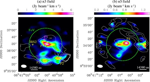
In this paper, we present mapping observations toward two positions in the NGC 2264-D cluster-forming region conducted by the Atacama Compact Array (ACA). The two positions, n3 and n5, were identified based on HC3N emission by Taniguchi et al. (2020b) (see figure 1). The n3 position is located at the northern edge of NGC 2264-D and the integrated intensity ratio of HC3N and CH3OH, I(HC3N)|$/$|I(CH3OH), at this position shows the highest value among the other positions in NGC 2264-C and NGC 2264-D. A variety in the I(HC3N)|$/$|I(CH3OH) ratio implies a chemical differentiation in the cluster-forming region, suggestive of different evolutionary histories and/or different environments (Spezzano et al. 2016, 2020; Taniguchi et al. 2019a). The n3 position is located to the west of the IRS2 source (IRAS 06382|$+$|0939). The n5 position lies at the southern part of the NGC 2264-D cluster-forming clump and shows the highest column density ratios of N2H+/CCS and N2H+/HC3N among the other positions in NGC 2264-D, which means that the n5 position is the most chemically evolved position in this cluster-forming clump. In section 2, the observations and reduction procedures are described. The dust continuum (λ = 3 mm) and moment 0 maps of molecular lines are presented in subsection 3.1, and spectra are shown in subsection 3.2. We analyze spectra using the CASSIS software (Vastel et al. 2015) in subsection 3.3. We compare spatial distributions of HC3N and CH3OH, and chemical compositions of the n3 field, the n5 field, and CMM3 in NGC 2264-C, in subsections 4.1 and 4.2, respectively. The main conclusions of this paper are summarized in section 5.
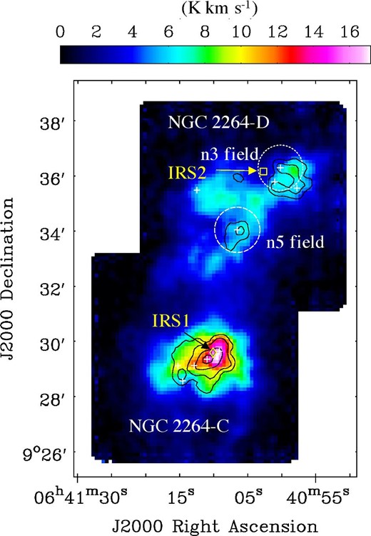
Moment 0 maps of HNC (J = 1–0) and HC3N (J = 10–9) lines, as shown in the color scale and black contours, respectively, toward the NGC 2264-C and NGC 2264-D cluster-forming clumps obtained with the Nobeyama 45 m telescope (Taniguchi et al. 2020b). Black contour levels are |$15\%$|, |$25\%$|, |$50\%$|, |$75\%$|, and |$90\%$| of the peak intensity (6.65 K km s−1). The white dashed circles represent the FoV of the ALMA ACA data (97|$^{\prime\prime} $|) presented in this paper. The white crosses indicate positions analyzed by Taniguchi et al. (2020b). (Color online)
2 Observations and data reduction
We analyzed the ALMA ACA Cycle 7 data in Band 3 toward the n3 and n5 positions in the NGC 2264-D cluster-forming clump.1 Figure 1 shows the moment 0 map of HNC (color scale) overlaid by the HC3N moment 0 map (black contours) toward the NGC 2264-C and NGC 2264-D cluster-forming clumps, as obtained with the Nobeyama 45 m radio telescope (Taniguchi et al. 2020b). The white dashed circles indicate fields observed by the ALMA ACA observations.
The ALMA ACA observations were carried out between 2020 January 1 and January 16. The phase reference centers were |$(\alpha _{\rm J2000.0}, \delta _{\rm J2000.0}) = ({6^{\rm h}41^{\rm m}00{^{\rm s}_{.}}16},{+9{^{\circ}_{.}}36^{\prime }18.^{\prime \prime }0})$| and |$({6^{\rm h}41^{\rm m}06{^{\rm s}_{.}}52},{+9{^{\circ}_{.}}34^{\prime }03.^{\prime \prime }1})$| for the n3 and n5 positions, respectively. Hereafter, we call each field of view the “n3 field” and “n5 field,” respectively. The phase calibrator source was J0643+0857 during all of the observations. For bandpass and flux calibrations, J0725−0054 and J0854+2006 were observed during the n3 observations, and only J0725−0054 was observed during the n5 observations. The field of view (FoV) and maximum recoverable scale (MRS) are ∼97|$^{\prime\prime} $| and ∼65|$^{\prime\prime} $|, respectively.
Table 1 summarizes information for each spectral window. The bandwidth and frequency resolution for the continuum observation are 1875 MHz and 1.129 MHz, respectively. The bandwidths are 58.59 MHz and 117.19 MHz for the spectral window including the CH3OH lines, and the spectral windows including the other lines (HC3N and CH3CN), respectively. The frequency resolution for these molecular lines is ∼141 kHz, corresponding to a velocity resolution of ∼0.38–0.44 km s−1.
Summary of spectral windows.
| Species | Transition | Frequency range | Frequency resolution |
|---|---|---|---|
| (GHz) | (MHz) | ||
| Continuum* | 97.6068–99.5591 | 1.129 | |
| CH3OH | 2−1, 2–1−1, 1 E | 96.7088–96.7697 | 0.141 |
| 20, 2–10, 1 A+ | |||
| HC3N | J = 12–11 | 109.097–109.219 | 0.141 |
| CH3CN | J = 6–5, K = 0, 1 | 110.300–110.422 | 0.141 |
This spectral window contains the CS, SO, and CH3CHO lines.
We conducted data reduction and imaging using the Common Astronomy Software Application (CASA v5.6.1; McMullin et al. 2007) on the pipeline-calibrated visibilities. The data cubes were made with the CASA tclean task. Uniform weighting was applied. The resulting angular resolution is approximately 17|$^{\prime\prime} $| × 11|$^{\prime\prime} $|, corresponding to ∼0.059 pc × 0.038 pc (∼12200 au × 7900 au) at the source distance (719 pc; Maíz Apellániz 2019). The pixel size and image size are |${2{^{\prime \prime}_{.}}5}$| and 250 × 250 pixels, respectively. Continuum (λ = 3 mm) images were created from the data cubes using the IMCONTSUB task. The polynomial order of 0 was adopted for the continuum estimation. The noise levels of the continuum images are 1.0 mJy beam−1 and 0.9 mJy beam−1 at the n3 and n5 fields, respectively.
3 Results and analyses
3.1 Continuum and moment 0 maps
Figure 2 shows the continuum (λ = 3 mm) images with a primary beam correction toward the two positions in NGC 2264-D. Panels (a) and (b) of figure 2 indicate the n3 and n5 fields, respectively. One prominent continuum core is located at the position northwest of the field of view in the n3 field. This core corresponds to DMM6 as identified by Peretto, André, and Belloche (2006) using the 1.2 mm dust continuum data. Additionally, the DMM4 and DMM15 cores have been detected in the n3 field. No continuum core was detected at the position of IRS2 (Class I YSO), which is consistent with the 1.2 mm dust continuum data.
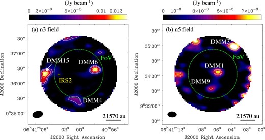
Continuum (λ = 3 mm) images with a primary beam correction toward (a) the n3 field and (b) the n5 field in the NGC 2264-D cluster-forming clump. The color scales are adjusted to the maximum values for the peak of clumps in the FoV. The contour levels are 5, 7, 10, and 12 σ for panel (a) and 5, 6, 7, 8, 9, and 10 σ for panel (b), where the noise levels are around 1.0 and 0.9 mJy beam−1 for panels (a) and (b), respectively. The green dashed circles represent FoV sizes (97′′). The yellow cross indicates the IRS2 (IRAS 06382+0939) position. The indications of “DMMn,” where n is a number, denote names of continuum cores identified by Peretto, André, and Belloche (2006). The filled black ellipses indicate angular resolutions of approximately |${16{^{\prime \prime}_{.}}6} \times {10{^{\prime \prime}_{.}}4}$| and |${17{^{\prime \prime}_{.}}6} \times {10{^{\prime \prime}_{.}}2}$| for panels (a) and (b), respectively. The linear scale is given for 30″ corresponding to 21570 au. (Color online)
In the n5 field, we adjust the color scale to the peak value for the DMM1 core. Two cores, DMM1 and DMM9 (Peretto et al. 2006), have been detected near the phase reference center. Since only a part of the brightest core (DMM3) is detected at the edge of the field, we do not include the DMM3 core in the following discussion.
Figure 3 shows moment 0 maps (with a primary beam correction) of molecular emission lines—HC3N (J = 12–11), CH3OH (the integrated frequency range covers three lines; 2−1, 2–1−1, 1 E, 20, 2–10, 1 A+, and 20, 2–10, 1 E, but the last line was detected only near the DMM1 core), CS (J = 2–1), SO (NJ = 32–21), and CH3CN (J = 6–5, K = 0, 1)—toward the n3 (the first and second rows) and n5 (the third and fourth rows) fields, respectively. The CH3CN maps have a different size from the others, because the moment 0 maps of CH3CN are noisier than the other maps, especially outside the FoV, and its emission is compact. We therefore show the close-up maps. Table 2 summarizes peak intensity and rms noise level for each panel. The CS and SO lines lie in the spectral window of the widest frequency coverage (table 1), and the velocity resolution of these lines is 3.43 km s−1. Such a low velocity resolution does not resolve the detected lines sufficiently, but we can identify these lines clearly. In the panel of CH3OH toward the n3 field, we adjust the color scale to the maximum value for the peak around the DMM4 continuum core so that its morphology in the field can be clearly seen. At the west edge where the CH3OH emission is saturated, the CH3OH lines show broad line features, suggestive of the shock regions, which may be the source of the high integrated intensity.
![Moment 0 maps of HC3N, CH3OH, CS, SO, and CH3CN toward the n3 (the first and second rows) and n5 (the third and fourth rows) fields in NGC 2264-D. The black contour levels are $20\%$, $40\%$, $60\%$, and $80\%$ of the peak intensities summarized in table 2 for panels of HC3N and CH3OH. For panels of CS, SO, and CH3CN, the black contour levels are [10, 15, 20, 25, 30 σ], [5, 7, 10, 13, 15, 17 σ], and [5, 6, 7, 8, 9 σ] in the n3 field, and [5, 7, 9, 11, 13 σ], [5, 6, 7, 8 σ], and [5, 6, 7 σ] in the n5 field, respectively. The rms noise levels for each panel are summarized in table 2. The integrated velocity ranges are (2, 9) km s−1 for HC3N, (−10, 18) kms−1 for CH3OH, (−10, 20) km s−1 for CS and SO, and (0, 14) km s−1 for CH3CN maps. The gray contours show the distribution of dust continuum emission, as in figure 2. The filled white ellipses represent the angular resolution (∼17″ × 11″). The yellow crosses indicate the IRS 2 and HC3N peak (P1–P4) positions, and the magenta cross in the n3 field indicates the CH3OH Peak (P5). The green dashed circles indicate the FoV. The linear scales are given for 20″ corresponding to 14380 au. (Color online)](https://oup.silverchair-cdn.com/oup/backfile/Content_public/Journal/pasj/73/6/10.1093_pasj_psab092/2/m_psab092fig3.jpeg?Expires=1749848524&Signature=rxOPw7vxDeLagMv25UmgA-2Y4SpDJUTYU81Bjgny3er3HRe7DqtXri~QI14CtNYGbPWWRdsztUKvS6NwxQAkgUHU1UUjgPGTGCI46mITF5uWL97HAAQ84KXQjG3qrl~1Slx1VdNREjdIaRp53zSpccgQNc5p~9AC0-YpYTrVBaIuJAtPQvnofP1FCxq8bgHigsHFpd1Ip19jXr8hBwYXtB1Ub-28LQH1Qo~5X4JFOcqPFT7iNCYdT9tnrVt9DWJ7LkXorLYb2cD~7Fqk6OfkkNkB6lBQudvG65eMOQ0hF9Z6mevesAexe~UyguIh3FOv00VBqsKFNddy5~~D8d6KRw__&Key-Pair-Id=APKAIE5G5CRDK6RD3PGA)
Moment 0 maps of HC3N, CH3OH, CS, SO, and CH3CN toward the n3 (the first and second rows) and n5 (the third and fourth rows) fields in NGC 2264-D. The black contour levels are |$20\%$|, |$40\%$|, |$60\%$|, and |$80\%$| of the peak intensities summarized in table 2 for panels of HC3N and CH3OH. For panels of CS, SO, and CH3CN, the black contour levels are [10, 15, 20, 25, 30 σ], [5, 7, 10, 13, 15, 17 σ], and [5, 6, 7, 8, 9 σ] in the n3 field, and [5, 7, 9, 11, 13 σ], [5, 6, 7, 8 σ], and [5, 6, 7 σ] in the n5 field, respectively. The rms noise levels for each panel are summarized in table 2. The integrated velocity ranges are (2, 9) km s−1 for HC3N, (−10, 18) kms−1 for CH3OH, (−10, 20) km s−1 for CS and SO, and (0, 14) km s−1 for CH3CN maps. The gray contours show the distribution of dust continuum emission, as in figure 2. The filled white ellipses represent the angular resolution (∼17″ × 11″). The yellow crosses indicate the IRS 2 and HC3N peak (P1–P4) positions, and the magenta cross in the n3 field indicates the CH3OH Peak (P5). The green dashed circles indicate the FoV. The linear scales are given for 20″ corresponding to 14380 au. (Color online)
Summary of moment 0 maps.
| Field | Species | Peak* | rms* |
|---|---|---|---|
| n3 | HC3N | 6.29 | 0.1 |
| CH3OH | 18.1 | 1.0 | |
| CS | 16.7 | 0.5 | |
| SO | 11.5 | 0.5 | |
| CH3CN | 0.55 | 0.05 | |
| n5 | HC3N | 1.34 | 0.05 |
| CH3OH | 6.59 | 0.3 | |
| CS | 4.3 | 0.3 | |
| SO | 2.4 | 0.2 | |
| CH3CN | 0.3 | 0.04 |
| Field | Species | Peak* | rms* |
|---|---|---|---|
| n3 | HC3N | 6.29 | 0.1 |
| CH3OH | 18.1 | 1.0 | |
| CS | 16.7 | 0.5 | |
| SO | 11.5 | 0.5 | |
| CH3CN | 0.55 | 0.05 | |
| n5 | HC3N | 1.34 | 0.05 |
| CH3OH | 6.59 | 0.3 | |
| CS | 4.3 | 0.3 | |
| SO | 2.4 | 0.2 | |
| CH3CN | 0.3 | 0.04 |
Unit is Jy beam−1 km s−1.
We identified three and one HC3N clumps in the n3 and n5 fields, respectively, and they are labelled as P1–P4. In the n3 field, we picked up the three clumps with a peak intensity greater than 4 Jy beam−1 km s−1. We applied 2D Gaussian fitting to the HC3N moment 0 maps. The fit results are summarized in table 3. P1, P2, and P3 in the n3 field correspond to n3, n2, and n4 positions, respectively, and P4 corresponds to the n5 position identified by Taniguchi et al. (2020b). The HC3N emission is not coincident with the strongest dust continuum core (DMM6) in the n3 field, whereas the HC3N emission is associated with the strongest 3 mm continuum core, DMM1, in the n5 field. P3 is associated with the DMM4 dust continuum core, but P2 does not seem to coincide with the dust continuum core in the n3 field. In the n5 field, a tail-like feature, which is elongated in the eastern direction, is associated with the P4 peak, and a weaker peak was seen at the east position. Another weaker HC3N emission is associated with the DMM9 core. The diffuse HC3N emission appears to bridge DMM1 and DMM9.
Summary of 2D Gaussian fitting for the HC3N moment 0 maps.
| Name | Peak position (J2000.0) | Size* | Position angle | Peak intensity |
|---|---|---|---|---|
| (Jy beam−1 km s−1) | ||||
| P1 | |${6^{\rm h}41^{\rm m}00{^{\rm s}_{.}}021}\, \pm \, {0{^{\rm s}_{.}}039}$|, |${+9{^{\circ}}36^{\prime }17.^{\prime \prime }92} \pm {0{^{\prime \prime}_{.}}25}$| | |${30{^{\prime \prime}_{.}}59} \pm {1{^{\prime \prime}_{.}}63} \times {11{^{\prime \prime}_{.}}78} \pm {0{^{\prime \prime}_{.}}67}$| | |${69{_{.}^{\circ}}6} \pm {2{_{.}^{\circ}}0}$| | 6.06 ± 0.21 |
| P2 | |${6^{\rm h}40^{\rm m}57{^{\rm s}_{.}}868} \pm {0{^{\rm s}_{.}}051}$|, |${+9{^{\circ}}35^{\prime }34.^{\prime \prime }48} \pm {0{^{\prime \prime}_{.}}38}$| | |${20{^{\prime \prime}_{.}}9} \pm {2{^{\prime \prime}_{.}}4} \times {13{^{\prime \prime}_{.}}8} \pm {1{^{\prime \prime}_{.}}5}$| | |${97^{\circ}} \pm {14^{\circ}}$| | 4.42 ± 0.27 |
| P3 | |${6^{\rm h}41^{\rm m}00{^{\rm s}_{.}}544} \pm {0{^{\rm s}_{.}}074}$|, |${+9{^{\circ}}35^{\prime }28.^{\prime \prime }77} \pm {0{^{\prime \prime}_{.}}35}$| | |${34{^{\prime \prime}_{.}}7} \pm {2{^{\prime \prime}_{.}}9} \times {13{^{\prime \prime}_{.}}3} \pm {1{^{\prime \prime}_{.}}1}$| | |${96{_{.}^{\circ}}8} \pm {2{_{.}^{\circ}}9}$| | 4.13 ± 0.23 |
| P4 | |${6^{\rm h}41^{\rm m}05{^{\rm s}_{.}}895} \pm {0{^{\rm s}_{.}}034}$|, |${+9{^{\circ}}34^{\prime }04.^{\prime \prime }18} \pm {0{^{\prime \prime}_{.}}29}$| | |${23{^{\prime \prime}_{.}}94} \pm {1{^{\prime \prime}_{.}}52} \times {17{^{\prime \prime}_{.}}38} \pm {0{^{\prime \prime}_{.}}98}$| | |${95{_{.}^{\circ}}3} \pm {9{_{.}^{\circ}}1}$| | 1.27 ± 0.05 |
Reported results are deconvolved sizes, which take into account the synthesized beam.
The CH3OH spatial distributions are different from those of HC3N in both fields. In the n3 field, an elongated feature is seen around P3. Two CH3OH peaks in this structure are not coincident with the P3 HC3N peak. The CH3OH emission seems to be spatially anti-correlated with the DMM6 continuum core. The CH3OH emission is weak at the dust continuum peak. We determined a CH3OH peak by eye and named it P5, which is located near P1, as shown in the panel of the n3 field. The coordinate of the P5 position is |$(\alpha _{\rm J2000.0}, \delta _{\rm J2000.0}) = ({6^{\rm h}41^{\rm m}00{^{\rm s}_{.}}78}, {+9{^{\circ}_{.}}36^{\prime }29.^{\prime \prime }88})$|. The emission near P3 likely originates from the molecular outflow due to strong wing emission (figure 6), and therefore the comparison of chemical composition focuses on the region around P5 instead. In the n5 field, the CH3OH emission is associated with the DMM1 continuum core, but does not coincide exactly with the dust peak position. In addition, a strong peak is located to the west of the DMM1 core.
The SO (32–21; 99.299905 GHz) emission shows an elongated feature in the north-eastern to south-western direction, centering on the DMM6 core. Such a feature resembles the CH3OH emission. The CS (J = 2–1; 97.980953 GHz) emission shows strong emission near the DMM6 core. Both CS and SO show strong features at the edge of the field near P2, which is consistent with the CH3OH emission. In addition, the CS and SO emission have been detected at P3 and at a position east of IRS2. In the n5 field, the spatial distributions of CS and SO emission lines are roughly similar to that of CH3OH.
The last panels of figure 3 shows moment 0 maps of CH3CN. Its peak positions are consistent with the P1 and P4 HC3N peaks in the n3 and n5 fields, respectively. In the n3 field, another core is found to the west of P1, and weak emission is associated with the DMM6 core.
Two CH3CHO lines, 51, 4–41, 3 E (98.8633135 GHz; Eup = 16.6 K) and 51, 4–41, 3 A− (98.9009445 GHz; Eup = 16.5 K), have been detected toward the n5 field in the spectral window with the widest frequency band (continuum observations; table 1). Figure 4 shows its moment 0 map (51, 4–41, 3 E) and spectra of the two lines toward its peak position, determined by eye and indicated as “CH3CHO peak” in the moment 0 map. The coordinate of the CH3CHO peak is |$(\alpha _{\rm J2000.0}, \delta _{\rm J2000.0}) = ({6^{\rm h}41^{\rm m}06{^{\rm s}_{.}}821}, {+9{^{\circ}_{.}}33^{\prime }53.^{\prime \prime }05})$|. The spectra are obtained by averaging over pixels within the 10″ diameter centered at the CH3CHO peak. The CH3CHO emission is detected within the CH3OH emitting region.
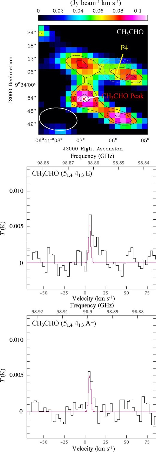
Top panel: Moment 0 map of CH3CHO (51, 4–41, 3 E) toward the n5 field. The contour levels are 3, 4, and 5 σ. The noise level is 0.02 Jy beam−1 km s−1. The integrated velocity range is 0–+24 km s−1. The open white ellipses represent an angular resolution of |${17{^{\prime \prime}_{.}}4}\times {10{^{\prime \prime}_{.}}3}$|. The P4 position indicates the HC3N peak position. Middle and bottom panels: Spectra of the CH3CHO lines toward the CH3CHO peak. The spectra are obtained by averaging over pixels within the 10″ diameter (7190 au) centered at the CH3CHO peak. The rms noise level of these spectra is ∼2 mK. The purple curves indicate the fitting results with the CASSIS software (subsection 3.3). (Color online)
3.2 Spectra
Figures 5 and 6 show the spectra of HC3N and CH3OH, respectively, at positions P1–P5, as well as the CH3CHO peak. The CH3CN spectra at P1 and P4 are shown in figure 7. The spectra are obtained by averaging over pixels within the 15″ diameter (∼10800 au) at the centers of P1–P5 peak positions (table 3), and 10″ diameter (7190 au) centered at the CH3CHO peak, respectively. The beam size of 15″ corresponds to the clump size obtained by the 2D Gaussian fitting (table 3).
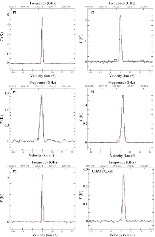
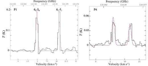
Spectra of the HC3N (J = 12–11; 109.173634 GHz) line toward the P1–P5 and CH3CHO peak positions. The spectra are obtained by averaging over pixels within the 15″ diameter (∼10800 au) at the centers of the P1–P5 peak positions (table 3) and the 10″ diameter (7190 au) centered at the CH3CHO peak, respectively. The rms noise level of these spectra is ∼10 mK and ∼5 mK in the n3 and n5 fields, respectively. Purple curves indicate the fitting results using the CASSIS software (subsection 3.3). (Color online)
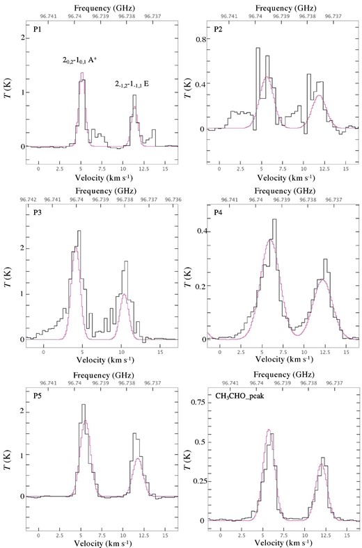
Spectra of the CH3OH (2−1, 2–1−1, 1 E; 96.739358 GHz, and 20, 2–10, 1 A+; 96.741371 GHz) lines toward the P1–P5 and CH3CHO peak positions. The spectra are obtained by averaging over pixels within the 15″ diameter (∼10800 au) at the centers of P1–P5 peak positions (table 3) and the 10″ diameter (7190 au) centered at the CH3CHO peak, respectively. The rms noise level of these spectra is ∼9 mK and ∼3 mK in P1 and P4, respectively. Purple curves indicate the fitting results using the CASSIS software (subsection 3.3). (Color online)
Spectra of the CH3CN (JK = 60–50; 110.3835 GHz, and 61–51; 110.381372 GHz) lines toward the P1 and P4 positions. The spectra are obtained by averaging over pixels within the 15″ diameter (∼10800 au) at the centers of P1 and P4 peak positions (table 3). The rms noise level of these spectra is ∼9 mK and ∼4 mK in the n3 and n5 fields, respectively. Purple curves indicate the fitting results using the CASSIS software (subsection 3.3). (Color online)
The HC3N spectra show narrow line features (figure 5). A weak wing emission is detected at the P4 position. The line widths of CH3CN are also narrow and comparable with those of HC3N. Since these lines have low upper-state energies (Eup = 18.5 K and 25.7 K for the K = 0 and K = 1 lines, respectively), they seem to originate from outer envelopes, rather than hot core regions close to protostars.
The CH3OH spectra show two velocity components at the P1 position, with a broad line feature or wing emission, as seen in figure 6. While the second velocity component may be detected at P2, the current noise level is not low enough to confirm it. The strong wing emission has been detected at P3. These results support the premise that the observed CH3OH lines trace shock regions. The missing fluxes were estimated at |$\sim\!\!10\%$| and |$\sim\!\!30\%$| in the n3 and n5 fields, respectively, determined by comparisons to the CH3OH data obtained with the Nobeyama 45 m telescope (Taniguchi et al. 2020b).
3.3 Spectral analysis with CASSIS
We analyzed spectra of HC3N (figure 5), CH3OH (figure 6), and CH3CN (figure 7) with the CASSIS software (Vastel et al. 2015) and the Jet Propulsion Laboratory (JPL) spectroscopic database.2 Since we have only one or two lines with similar upper-state energies for each species, we applied the Markov chain Monte Carlo (MCMC) method assuming the local thermodynamic equilibrium (LTE) model available in CASSIS. In the MCMC method, the minimum and maximum values set for a parameter in a component define the bounds in which the values are chosen randomly. The column density (N), excitation temperature (Tex), line width (FWHM), and radial velocity (VLSR) were derived and treated as semi-free parameters within certain ranges. CASSIS iteratively proceeds through a given parameter space via a random walk and reaches the final solution by a χ2 minimization.3
Taking previous observational results of Tex of N2H+ with a beam size of 18″ (∼10–26 K; Taniguchi et al. 2020b), we set the range of Tex between 10 and 40 K so that this Tex range fully covers the range of the N2H+ excitation temperature in the NGC 2264-D cluster-forming region. The ranges of other parameters are summarized in table 6 in the Appendix.
Table 4 summarizes results derived by the MCMC method. Since parts of the P2 and P3 clumps are located outside the FoV, the derived column densities can be erroneous, and we omit a quantitative discussion from the remainder this paper. The derived Tex values are consistent with Tex of N2H+ derived by the Nobeyama 45 m observations at each position. As a test, we ran the program several times and compared the results. We found that the derived column densities change within their errors, which is the major uncertainty in our discussion (section 4). In addition, we should note that it is common to determine the column density and Tex simultaneously from more than one molecular transition line. In order to check how nicely the MCMC analysis works, we independently applied the method to the HC3N (J = 10–9) data obtained by the Nobeyama 45 m telescope (Taniguchi et al. 2020b) and the HC3N (J = 12–11) data convolved to the same angular resolution (21′′). Resulting values of Tex for the two transitions are consistent with each other, though Tex for HC3N (J = 10–9) is slightly lower than that for HC3N (J = 12–11) by ∼4 K, which may be due to the missing flux of ACA data and slight differences of upper state energies.
Summary of analytical results.*
| Position | N | Tex | FWHM | VLSR |
|---|---|---|---|---|
| (cm−2) | (K) | (km s−1) | (km s−1) | |
| HC3N | ||||
| P1 | 1.7 (0.9) × 1013 | 14 (3) | 0.82 (0.19) | 4.77 (0.21) |
| P2 | 1.1 (0.7) × 1013 | 15 (3) | 0.77 (0.13) | 4.86 (0.36) |
| P3 | 1.9 (0.7) × 1013 | 13 (2) | 1.40 (0.19) | 4.49 (0.09) |
| P4 | 2.0 (0.9) × 1012 | 25 (4) | 1.03 (0.17) | 5.84 (0.27) |
| P5 | 9.4 (3.5) × 1012 | 14 (2) | 0.87 (0.17) | 4.99 (0.07) |
| CH3CHO peak | 1.7 (0.9) × 1012 | 17 (3) | 0.89 (0.13) | 5.68 (0.58) |
| CH3OH† | ||||
| P1 | 1.1 (0.3) × 1014 | 15 (2) | 0.96 (0.13) | 5.16 (0.10) |
| P2 | 2.4 (0.3) × 1014 | 32 (3) | 1.87 (0.12) | 5.60 (0.06) |
| P3 | 1.4 (0.4) × 1014 | 15 (4) | 1.11 (0.20) | 3.98 (0.14) |
| P4 | 2.8 (0.5) × 1014 | 34 (5) | 2.78 (0.20) | 5.89 (0.06) |
| P5 | 2.5 (0.9) × 1014 | 16 (3) | 1.33 (0.16) | 5.43 (0.24) |
| CH3CHO peak | 1.2 (0.7) × 1014 | 23 (4) | 1.84 (0.33) | 5.07 (0.52) |
| CH3CN | ||||
| P1 | 4.5 (1.0) × 1011 | 19.9 (5.1) | 0.66 (0.08) | 4.9‡ |
| P4 | 2.9 (0.4) × 1011 | 29.2 (1.3) | 0.85 (0.14) | 5.97 (0.05) |
| CH3CHO† | ||||
| CH3CHO peak | 6.0 (2.4) × 1011 | 26 (9) | 2.11 (0.69) | 5.04 (0.54) |
Numbers in parentheses are the standard deviation.
Both A-type and E-type are taken into consideration, assuming the same column density for both types.
The fitting was done with the fixed radial velocity.
We also analyzed the CH3CHO spectra with the same method (figure 4). The results of the Gaussian fitting do not seem to match the spectral shape perfectly, although we also note that the velocity resolution of the observations is 3.43 km s−1, and better resolution is needed to reveal finer details for a better fit.
4 Discussion
As seen in subsection 3.1, the spatial distributions of CH3OH are different from those of HC3N in NGC 2264-D. In subsection 4.1, we will compare their spatial distributions in detail. We further compare chemical compositions among the n3 field, the n5 field, and NGC 2264-C in subsection 4.2.
4.1 Comparison of spatial distributions of HC3N and CH3OH
Figure 8 shows comparisons of spatial distributions between CH3OH and HC3N toward (a) the n3 field and (b) the n5 field, respectively. In the n3 field, three HC3N peaks, P1–P3, are not coincident with the CH3OH emission peaks. A bright knot and extended west-facing bow shock, labeled as MHO 1385 by Buckle, Richer, and Davis (2012), was identified in an H2 map at the exact position of P1. Buckle, Richer, and Davis (2012) mentioned that the detection of the bright knot and bow shock indicates the presence of protostar(s). Thus, the CH3OH emission seems to come from shock regions induced by the jet or molecular outflows originating from protostar(s) embedded in the DMM6 core or the P1 clump.
Comparison of moment 0 maps between HC3N (color) and CH3OH (white contours), as in figure 3, toward (a) the n3 field and (b) the n5 field, respectively. (Color online)
The P2 position is located at the edge of the CH3OH emission peak. At this edge of the FoV, the line widths of CH3OH are significantly broad, and the strong SO and CS lines are detected. Thus, the CH3OH emission is likely associated with a shock region. Although we could not identify the origin of the HC3N emission to be exactly at P2, it is likely that the HC3N emission is associated with a Spitzer source (YSO) identified at |${2{^{\prime \prime}_{.}}86}$| from the P2 peak position (Rapson et al. 2014).
The P3 clump corresponds to the dust clump No. 8 in Buckle and Richer (2015), identified using the 850 μm continuum emission. This clump contains a Class II protostar (Buckle & Richer 2015). In addition, Shimoikura et al. (2018) identified an infrared (IR) cluster at the P3 clump position (4753cl1). At the P3 position, the HC3N peak is located between two CH3OH peaks. These features indicate that the warm gas around a YSO is traced by the HC3N emission, while the molecular outflows are traced by the low upper-state-energy lines of CH3OH.
In the n5 field, the P4 position is located at the edge of the CH3OH emission. The HC3N peak (P4) is consistent with the DMM1 dust continuum core (figure 3). As seen in the CH3OH spectra (figure 6), the CH3OH spectra have wide line widths (table 4) and probably show a broadened wing emission. The HC3N spectra at P4 shows weak wing emission (figure 5) and a wider line width compared to the other positions (table 4). These results indicate that HC3N is associated with protostellar cores, and some emission may come from the molecular outflow, while the CH3OH emission prefers to trace the molecular outflow rather than hot cores. Protostars are likely being formed in the P4 clump, because Buckle, Richer, and Davis (2012) identified compact knots and fingers (MHO 1388) at the P4 peak. Furthermore, both Class 0/I and II protostars have been identified in this clump (Buckle & Richer 2015). An IR cluster was also identified (4753cl2; Shimoikura et al. 2018). Hence, this position can be considered as an active star formation site. These protostars should produce turbulent gas, and shock regions can be invoked.
In summary, the CH3OH emission seems to trace shock regions that the HC3N emission does not trace. In fact, the CH3OH spectra at P1–P3 shows, marginally, either two velocity components or a wing emission (figure 6). On the other hand, the HC3N emission seems to trace more quiescent regions. The HC3N emission associated with clumps containing low-mass YSOs has been reported in other YSOs (e.g., Taniguchi et al. 2021). The detection of CH3OH has been reported in the molecular outflows associated with some YSOs (Bachiller et al. 1998; Gibb & Davis 1998; Garay et al. 2000). These results support our suggestion that the CH3OH lines detected in the NGC 2264-D cluster-forming clump mainly trace shock regions. Furthermore, Holdship et al. (2019) detected CH3CHO in the molecular outflows of NGC 1333-IRAS2A, NGC 1333-IRAS4A, and L1157, besides CH3OH. The spatial coincidence of CH3CHO and CH3OH in the P4 clump suggests that the CH3CHO emission also originates from the molecular outflow.
The turbulent gas seems to be produced by the star formation activity in the NGC 2264-D cluster-forming clump. Hence, the star formation activity, in particular the jet and the molecular outflow, significantly affects the larger-scale (∼0.1 pc) chemistry.
4.2 Comparison of chemical composition between NGC 2264-D and NGC 2264-C
We derived the abundances of HC3N, CH3CN, and CH3CHO with respect to CH3OH in NGC 2264-D, as summarized in table 5. We also derived these values toward CMM3 in NGC 2264-C using observational results from Watanabe et al. (2015). The beam sizes of their observations were 15′′–22′′, which are comparable with the scale being discussed in this paper. We adopted the CH3OH column density of the “cold component,” (1.8 ± 0.2) × 1015 cm−2, because its excitation temperature of ∼25 K is closer to our results (table 4). Even if we adopt the total CH3OH column density of (2.1 ± 0.2) × 1015 cm−2 (Watanabe et al. 2015), our results and discussions do not change significantly. Missing flux may be present in our ACA data. Since we do not have single-dish data of the same transition except for CH3OH, we cannot derive missing flux for each line. However, we can compare chemical compositions among different sources using the column density ratios, which will reduce the effect of the missing flux.
Summary of the column density ratios with respect to methanol at each position in the NGC 2264 cluster-forming clumps.*
| Position | HC3N|$/$|CH3OH | CH3CN|$/$|CH3OH | CH3CHO|$/$|CH3OH |
|---|---|---|---|
| P1 | 0.160 ± 0.102 | 0.004 ± 0.002 | ... |
| P4 | 0.007 ± 0.003 | 0.0010 ± 0.0002 | ... |
| P5 | 0.038 ± 0.021 | ... | ... |
| CH3CHO peak | 0.014 ± 0.011 | ... | 0.005 ± 0.004 |
| NGC 2264-C† | 0.089 ± 0.019 | 0.008 ± 0.002 | 0.043 ± 0.007 |
The errors are calculated from the standard deviation of the column densities.
The column densities are taken from Watanabe et al. (2015); N(HC3N) = (1.6 ± 0.3) × 1014 cm−2, N(CH3OH) = (1.8 ± 0.2) × 1015 cm−2, N(CH3CN) = (1.5 ± 0.4) × 1013 cm−2, and N(CH3CHO) = (7.7 ± 0.8) × 1013 cm−2.
Figure 9 shows comparisons of the abundances of three molecules with respect to CH3OH in the NGC 2264 cluster-forming clumps. The top panel shows the HC3N case. As mentioned in section 1, the HC3N|$/$|CH3OH abundance ratio is a tracer to investigate evolutionary stages of YSOs and environment. The HC3N|$/$|CH3OH ratios in the n3 field have larger values than those in the n5 field systematically. The HC3N abundance is likely less sensitive to protostellar evolution compared to CH3OH, because HC3N is continually formed from CH4 and/or C2H2, which are sublimated from dust grains, in warm or hot regions (25 K < T < 100 K) (e.g., Taniguchi et al. 2019a). Thus, these results imply that CH3OH is efficiently sublimated from dust grains in the n5 field.
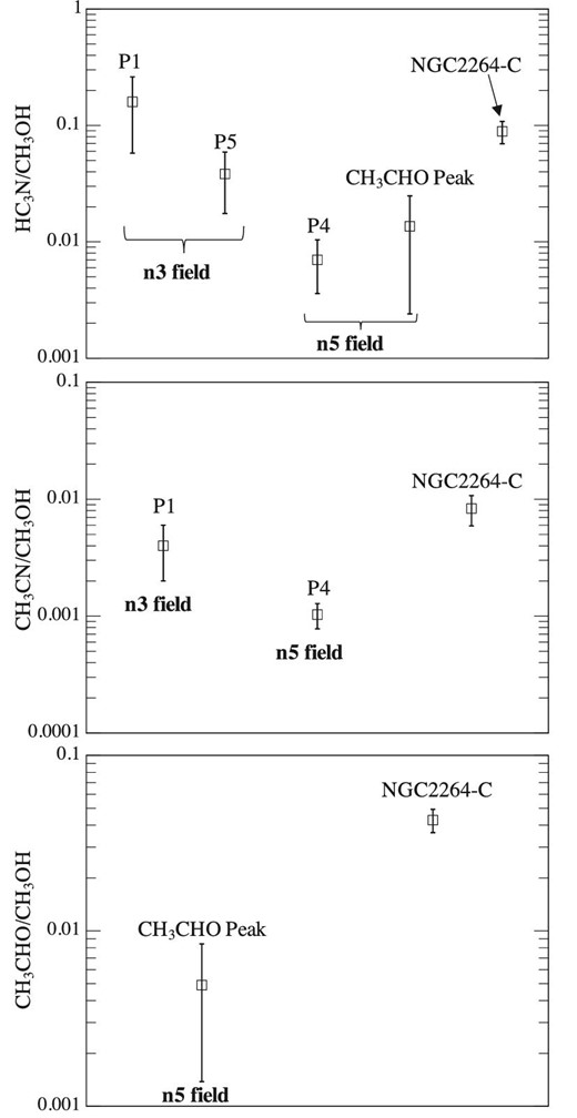
Comparisons of chemical composition in the NGC 2264 cluster-forming clumps. Top, middle, and bottom panels show the HC3N|$/$|CH3OH ratio, the CH3CN|$/$|CH3OH ratio, and the CH3CHO|$/$|CH3OH ratio, respectively.
In order to confirm this hypothesis, we investigated the relationship between the excitation temperatures of HC3N and CH3OH, Tex(HC3N), and Tex(CH3OH), and the HC3N|$/$|CH3OH ratio, as shown in figure 10. Since there are not enough data points, we could not conduct statistical tests. However, both panels of figure 10 show a similar tendency; the HC3N|$/$|CH3OH ratio decreases as their excitation temperatures increase. Even if there are uncertainties in deriving the column densities (subsection 3.3) and the missing flux, this main conclusion does not change, because differences in the HC3N|$/$|CH3OH abundance ratios between n3 and n5 are around one order of magnitude.
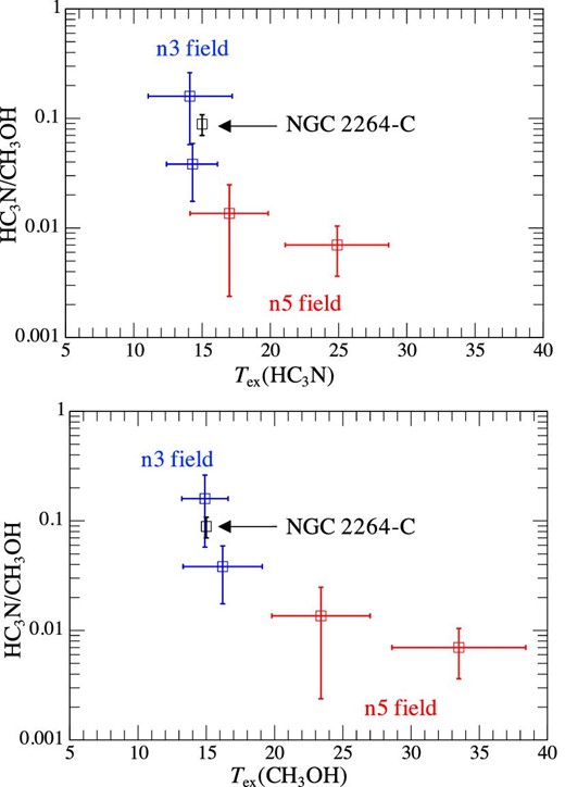
Relationship between the excitation temperature of HC3N and the HC3N|$/$|CH3OH column density ratio (upper panel). The lower panel shows the same, but the excitation temperature of CH3OH is used. The blue, red, and black points indicate the n3 field, the n5 field, and CMM3 in NGC 2264-C, respectively. (Color online)
The anti-correlations between the HC3N|$/$|CH3OH ratio and Tex indicate that CH3OH can be more efficiently sublimated from dust grains in warmer clumps. These results suggest not only that thermal sublimation occurs by heating from protostars, but also by heating of dust grains in turbulent regions, as well as by the effects of photons (i.e., the photon heating effect causing non-thermal desorption) (Taniguchi et al. 2021). Overall, the n5 field is a more active star formation site than the n3 field in terms of chemical compositions.
The middle panel of figure 9 shows a comparison of the CH3CN|$/$|CH3OH ratio at P1, P4, and CMM3 in NGC 2264-C. This ratio at the P4 position is lower than those at the others, and the ratio at P1 is similar to that at CMM 3 in NGC 2264-C. This tendency is the same as the HC3N case. Codella et al. (2009) derived the CH3CN|$/$|CH3OH column density ratio in the L1157-B1 clumps in the molecular outflow. The derived values in L1157 were (0.2–1.3) × 10−3, which is consistent with the value at P4 in the n5 field.
The bottom panel (figure 9) shows a comparison of the CH3CHO|$/$|CH3OH ratio at the CH3CHO peak and CMM3 in NGC 2264-C. Since we detected only two CH3CHO lines, there is a large uncertainty in the CH3CHO abundance. The CH3CHO|$/$|CH3OH ratio at the CH3CHO peak seems to be lower than that at CMM3 in NGC 2264-C, but similar to the values derived in molecular outflows [(0.8–6.7) × 10−3; Holdship et al. 2019]. The results of the CH3CN|$/$|CH3OH ratio at P4 and the CH3CHO|$/$|CH3OH ratio at the CH3CHO peak support the view that this region is a shock region induced by the molecular outflow.
From the point of view of chemical compositions, the P4 clump is a more active star-forming region than the others in NGC 2264-D. Taniguchi et al. (2020b) concluded that the n5 position is the most evolved in the NGC 2264-D cluster-forming clump by the combination of evolution along the filamentary structure and evolution of each clump. Using these ACA data, we found that the degree of star formation activities and the nature of environments are also different among clumps in the NGC 2264-D region in terms of chemical composition. In fact, the most active star forming clump, the P4 clump, contains Class 0/I and II sources, while there are only Class 0/I sources in the P1 and P2 clumps, and a Class II source in the P3 clump (Buckle & Richer 2015). The mixing of a variety of classes of YSOs seems to indicate the second round of star formation in the P4 clump. These results also support the view that the P4 clump in the n5 field is the most active ongoing star formation site.
Chemical compositions in cluster-forming clumps change from site to site. These results indicate that the stellar feedback or environments affect the chemical composition of the large clump scale. Although the n3 field is farther from NGC 2264-C compared to the n5 field, the chemical characteristics of the n3 field may be similar to those of CMM3 in NGC 2264-C. The current data set includes a limited number of molecules, and future line survey observations with higher angular resolution are needed to confirm similarities/differences of chemical characteristics, and to disentangle the complicated effects from each protostar.
5 Conclusions
We present the ALMA ACA Cycle 7 data in Band 3 toward the n3 and n5 fields in the NGC 2264-D cluster-forming region. The HC3N, CH3OH, and CH3CN lines were detected. In addition, the CS, SO, and CH3CHO emission lines were detected in a spectral window with the widest frequency coverage for the continuum observations.
We identified three and one HC3N emission peaks in the n3 and n5 fields, respectively. The strongest dust continuum core in the n3 field, DMM6, is not associated with the HC3N peak, while the P3 clump is consistent with the DMM4 continuum core. On the other hand, the spatial distributions of the observed CH3OH lines are similar to those of CS and SO. The P4 clump identified by the HC3N emission in the n5 field is consistent with the DMM1 continuum core. The CH3OH emission is also associated with the P4 clump, and its spectra show broad line widths and a wing emission, suggestive of a molecular outflow. In general, turbulent gas induced by star formation activities produces shock regions in NGC 2264-D. The sites of protostars are traced by the dust continuum and HC3N emission peaks.
We derived the HC3N, CH3CN, and CH3CHO abundances with respect to CH3OH. In general, chemical compositions in the n3 field are more similar to those at CMM3 in NGC 2264-C compared to the n5 field, despite the fact that the n3 field is farther from NGC 2264-C. We find anti-correlations between the HC3N|$/$|CH3OH abundance ratio and the excitation temperatures of HC3N and CH3OH. The lower HC3N|$/$|CH3OH ratio at the P4 clump in the n5 field seems to suggest that CH3OH is efficiently sublimated from dust grains by thermal or non-thermal heating. These results imply that the P4 clump is a more active star formation site than other clumps in the n3 field. This suggestion is supported by the fact that the P4 clump includes both Class 0/I and II sources, and the second round of star formation may have proceeded.
The clump scale chemistry seems to be significantly affected by star formation activities. Our results show that the clump-scale chemical composition is a key for understanding the evolution and environments of clumps.
Acknowledgements
This paper makes use of the following ALMA data: ADS/JAO.ALMA#2019.2.00030.S. ALMA is a partnership of ESO (representing its member states), NSF (USA) and NINS (Japan), together with NRC (Canada), MOST and ASIAA (Taiwan), and KASI (Republic of Korea), in cooperation with the Republic of Chile. The Joint ALMA Observatory is operated by ESO, AUI/NRAO and NAOJ. The National Radio Astronomy Observatory is a facility of the National Science Foundation operated under cooperative agreement by Associated Universities, Inc. Based on analyses carried out with the CASSIS software and JPL spectroscopic database. CASSIS has been developed by IRAP-UPS/CNRS 〈http://cassis.irap.omp.eu〉. This work was supported by Japan Society for the Promotion of Science (JSPS) KAKENHI grant No. JP20K14523. This work was supported in part by Japan Foundation for Promotion of Astronomy. E.H. thanks the National Science Foundation for support through grant AST-1906489. We thank the anonymous referee who gave us valuable comments, which helped us improve the quality of the paper.
Appendix. Parameter ranges used in the MCMC method
Table 6 summarizes the parameter ranges for the spectral analyses (subsection 3.3).
Summary of parameter ranges used in the MCMC method.*
| Species | N | FWHM | VLSR |
|---|---|---|---|
| (cm−2) | (km s−1) | (km s−1) | |
| HC3N | 5 × 10¹¹–5 × 10¹⁵ | 0.5–2.5 | 4.5–5.0 |
| CH3OH | 1 × 10¹¹–1 × 10¹⁶ | 0.5–3.0 | 3.5–6.0 |
| CH3CN | 1 × 10¹¹–1 × 10¹⁴ | 0.5–2.5 | 5.7–6.5 |
| CH3CHO | 1 × 10¹¹–1 × 10¹³ | 1.0–4.0 | 4.0–6.0 |
| Species | N | FWHM | VLSR |
|---|---|---|---|
| (cm−2) | (km s−1) | (km s−1) | |
| HC3N | 5 × 10¹¹–5 × 10¹⁵ | 0.5–2.5 | 4.5–5.0 |
| CH3OH | 1 × 10¹¹–1 × 10¹⁶ | 0.5–3.0 | 3.5–6.0 |
| CH3CN | 1 × 10¹¹–1 × 10¹⁴ | 0.5–2.5 | 5.7–6.5 |
| CH3CHO | 1 × 10¹¹–1 × 10¹³ | 1.0–4.0 | 4.0–6.0 |
The excitation temperature in the range 10–40 K is applied for all of the cases.
Footnotes
Project ID; 2019.2.00030.S, PI; Kotomi Taniguchi.
