Hoyle–Lyttleton accretion on to black hole accretion disks with super-Eddington luminosity for dusty gas

Abstract

1 Introduction

Revealing the formation and growth of black holes (BHs) is one of the central issues in astronomy. Recent observations have successfully detected several tens of stellar-mass BHs in our galaxy as X-ray binaries (Corral-Santana et al. 2016). However, considering the total stellar mass and the initial mass function, more BHs could have been formed in our galaxy up to the present day. Agol and Kamionkowski (2002) suggested that our galaxy might harbor a total of ∼10⁸–10⁹ BHs (see also Caputo et al. 2017). Recent observations have indicated isolated BHs might be floating in interstellar space (Sashida et al. 2013; Oka et al. 2016, 2017; Takekawa et al. 2017, 2019; Yamada et al. 2017). The isolated BHs can attract and swallow the gas while moving in interstellar space. This process is known as the Hoyle–Lyttleton accretion (Hoyle & Lyttleton 1939), and it plays a main role in the growth of BHs. In fact, Rice and Zhang (2021) and Safarzadeh and Haiman (2020) proposed that the gas accretion via the Bondi–Hoyle–Lyttloton mechanism may solve the mass gap problem pointed out by LIGO Scientific Collaboration (2020) and Liu and Lai (2021) from the detection of the gravitational wave. However, the spatial distribution of BHs and their growth mechanism have not been understood yet.

The study of the gas accretion on to a BH was initiated in the late 1930s (Hoyle & Lyttleton 1939; Bondi & Hoyle 1944; Bondi 1952). Subsequently, a detailed investigation was conducted using the hydrodynamics simulations (Shima et al. 1985; Ruffert & Arnett 1994; Ruffert 1996). These previous studies did not take into account the radiation force that changes the gas dynamics significantly as the source becomes bright. Therefore, the radiation hydrodynamic simulations of the gas accretion were performed recently with the assumption of an isotropic central source (Milosavljevic et al. 2009; Park & Ricotti 2011, 2012, 2013; Sugimura & Ricotti 2020; Toyouchi et al. 2021). When the accretion disk forms around BH, the radiation field is expected to be anisotropic. It allows the gas accretion from a shadow region, resulting in a higher accretion rate (e.g., Sugimura et al. 2017; Takeo et al. 2018).

The radiation hydrodynamics simulations are still an expensive way to investigate various parameters such as gas density, flow speed, and the anisotropy of radiation. Therefore the dependencies on the parameters are poorly understood. An alternative method is to solve the steady flow structure of the accreting gas, the low computational cost of which allows systematic study. Based on the analysis of the steady flow, Fukue and Ioroi (1999) examined the Hoyle–Lyttleton accretion around BH accretion disks with luminosities lower than the Eddington limit. They revealed that the accretion rate became small as the Eddington ratio increased, and the reduction rate could be more than |$70\%$|⁠, compared to the cases without the radiation feedback. Hanamoto, Ioroi, and Fukue (2001) calculated the Hoyle–Lyttleton accretion on to the super-Eddington disks. They showed that the self-shielding of the disk drastically reduces the radiation force, resulting in a high accretion rate even for the super-Eddington luminosity.

The above studies of the steady flow ignored interstellar dust. As star formation proceeds, galaxies become enriched with dust and metals. The dust-to-gas mass ratio is |$\sim 1\%$| in our galaxy (Zubko et al. 2004) and higher in quasars or ultraluminous infrared galaxies (Solomon et al. 1997). In such a situation, the radiation force on the dust has significant impacts on the gas accretion because of the higher absorption efficiency of dust (e.g., Yajima et al. 2017). In the case without dust, the radiation force on electrons simply decreases with the square of the distance from a source as the gravitational force in the rarefied plasma. On the other hand, the radiation force on dust also changes due to the dust attenuation, which makes the analysis of the flow structure complicated.

Thus, in this study, we investigate the steady structure of Hoyle–Lyttleton accretion of dusty gas with the radiative transfer considering the dust attenuation. For this purpose, the equation of motion, which incorporates the gravity of the BH and the radiation force by the BH accretion disk, is solved combined with the continuity equation. Here, we assume that the gas pressure is negligibly small since the velocity is larger than the sound velocity. However, this situation may change if the shock occurs. We will discuss shock waves in detail in subsection 4.3. As a result, we can evaluate the accretion rate in the situation where BHs are moving in the high-density dusty gas. This paper is organized as follows. In section 2 we introduce basic equations and describe the numerical method. In section 3 we show our simulation results, and section 4 is devoted to discussion. Finally, the summary and conclusion are given in section 5.

2 Basic equations and numerical method

2.1 Overview

We study a steady structure of flows around the BHs which are surrounded by the accretion disks and move in the dusty gas. The method for investigating the structure of the flow is similar to that used by Fukue and Ioroi (1999), but here we consider the extinction of the radiation from the accretion disks via the absorption by the dusty gas. The steady structure of the flows is given by the calculation of the trajectories of fluid elements (streamlines), which come towards the BHs from far enough away in the BH rest frame. We solve the equation of motion considering the radiation force as well as the gravity with the mass conservation along the streamline.

Figure 1 shows the configuration of the system. We use the cylindrical coordinates (r, ϕ, z) where the central BH is located at the origin. The accretion disk around the BH is small enough to be recognized as the point-like radiation source. The rotation axis of the disk is located on the plane of ϕ = 0, and the angle between the rotation axis and the z-axis is Θ. All streamlines are supposed to be parallel to the z-axis at the starting point of the streamlines, z = z_ini ≫ R_HL, where R_HL is the Hoyle–Lyttleton accretion radius. At the starting point, the density and the velocity of the flow are assumed to be uniform. When we solve for the ith streamline, the radiation from the central object is diluted via the absorption by the i′th (1 ≤ i′ < i) streamlines. We take into account the self-shielding by the ith flow. When the calculation of the final (outermost) streamline is finished, the global structure of the flow is obtained.

Fig. 1.

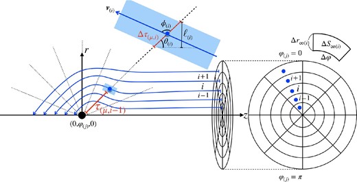
Configuration of the system. We adopt cylindrical coordinates (r, ϕ, z) and the BH accretion disk is located at the origin. The blue arrows indicate streamlines in the plane where phi is constant, and the blue point in the right circle is the starting points of the calculation of the streamlines. The optical depth is measured along radial dashed lines extending from the origin. The radiation force at the blue point on the ith streamline is calculated using the optical depth due to the streamlines up to the (i − 1)th, τ_{(m, i−1)}, and the optical depth of the ith streamline itself, Δτ_{(m, i)}. The large blue rectangle shows an enlarged view of the blue point on the ith streamline. Here, |$\boldsymbol{v}_{(i)}$| is the velocity vector of streamline, φ_(i) is the angle between velocity vector and position vector, θ_(i) is the polar angle measured from the z-axis, and |$l_{(i)}/\rm {sin}\theta _{(i)}$| is the path length as the photon passes through the ith streamline. (Color online)

Open in new tabDownload slide

At the point where the streamline reaches the z-axis behind the BH (z < 0), we check whether the condition for the accretion is satisfied or not. Using the streamlines which meet the condition, we evaluate the mass accretion rate on to the center, |$\dot{M}$|⁠. In subsection 2.3, the numerical method is described in more detail.

2.2 Basic equations

Since the accretion disk around the BH is recognized as the point source, and since the reprocessed radiation is neglected, only the R-component of the radiation flux (F_rad) is not zero. If the accretion disk is optically thick and geometrically thin, the radiation flux is evaluated as F_rad = Lcos ψe^−τ/2πR², where τ is the optical depth measured from the origin, L is the luminosity of the accretion disks, ψ is the angle from the rotation axis of the disk, and |$\cos \psi =|\boldsymbol{n}_{\rm rot} \cdot \boldsymbol{R}|/R$|⁠, with |$\boldsymbol{n}_{\rm rot}$| being the unit vector in the direction of the rotation axis. For comparison, we also consider the case of the isotropic radiation (isotropic model), F_rad = Le^−τ/4πR².

2.3 Numerical method

The right-hand part in figure 1 shows the cross-sectional view at z = z_ini. We calculate trajectories of the fluid element (streamlines) passing through the half of the circle (ϕ = 0 − π) with the radius R_HL since the flow is symmetric with respect to the ϕ = 0 plane (or ϕ = π plane). At z = z_ini, we suppose the dusty gas of uniform density flows in the z-direction. Hereafter the quantities at z = z_ini are denoted by the subscript ∞ as ρ_∞ and |$v^z_\infty$|⁠. We divide the half circle into 540 × 40 grid cells. The grid spacing in the r- and ϕ-directions is set to be constant; Δr = R_HL/540 and Δϕ = π/40, respectively. We calculate 540 × 40 trajectories of the fluid element (streamlines) by solving the equation (4) using the fourth-order Runge–Kutta method.

Since the ϕ component is zero in both radiation force and gravity, and since the r- and ϕ-components of the velocity is zero at z = z_ini, the fluid element movement on the plane of ϕ is constant. Thus, streamlines in the plane of ϕ = ϕ_(j) and those in the plane of |$\varphi =\varphi _{(j^{\prime }\ne j)}$| can be solved independently, where the subscript j denotes the number of grid points in the ϕ-direction (see figure 1). On the plane of ϕ = ϕ_(j), the initial position of the ith streamline is set to be (r, z) = (r_∞(i), z_ini), where r_∞(i) = (i − 0.5)Δr (the subscript i is the number of grid points in the r-direction). The cross-section at the initial point is ΔS_∞(i) = r_∞(i)ΔrΔϕ.

3 Result

3.1 Structure of flow

Figure 2 shows the velocity distribution and the ratio of radiation force to gravity of the pole-on model, Θ = 0 [panels (a)–(c)] and the isotropic model [panel (d)] for the case of τ_HL = 3.3, where τ_HL is defined as τ_HL = ρ_∞κ_dgR_HL. Here the vertical and horizontal axes indicate r/R_HL and z/R_HL, respectively. On the top half of the panel, the color contour indicates the velocity distribution and the yellow lines show the typical streamlines with i = 1, 70, 150, 230, 310, 390, and 470. The ratio of radiation force to gravity is plotted on the bottom half of the panel. We employ Γ′ = 0.6 [panel (a)], 3.0 [panels (b) and (d)], and 6.0 [panel (c)]. In both models, the flow is axisymmetric with respect to the z-axis.

Fig. 2.

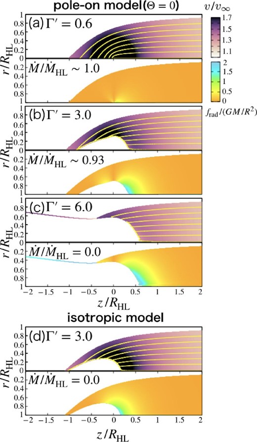
Velocity field (upper color contour) and the ratio of radiation force to gravity (lower color contour) of the pole-on model (a)–(c) and isotropic model for the case of τ_HL = 3.3 (d). The yellow lines overlaid in velocity distribution show the streamlines with i = 1, 70, 150, 230, 310, 390, and 470. We employ Γ′ = 0.6 (a), 3.0 (b and d), and 6.0 (c). (Color online)

Open in new tabDownload slide

In the sub-Eddington regime (Γ′ < 1.0), the gravity dominates over the radiation force in the whole region. This can be understood in the bottom half of figure 2a. It is found that most of the area is orange and the yellow region appears near the central region. Thus, the radiation force has little effect on the structure of the flow. In the top half of figure 2a, we see that the streamline, which is nearly parallel to the z-axis at z ≫ R_HL, is bent by the gravity of the BH and reaches the z-axis behind the BH (in the region of z < 0). The velocity increases near the central region due to the gravity of the BH. Most of the streamlines satisfy the accretion condition [see equation (9)], so that the accretion rate becomes |$\dot{M} \sim \dot{M}_{\rm HL} (\equiv \pi \rho _\infty v_\infty R_{\rm HL}^2 )$|⁠.

Even in the super-Eddington case (Γ′ > 1), the gas can accrete if the radiation force is weakened by attenuation. Figure 2b shows that the structure of the flow is not so different from that of figure 2a, except for the white region around the center. The 470th streamline (uppermost yellow line) is almost the same in figures 2a and 2b. This means that the radiation force is too weak to change the motion of the gas passing through the region far from the BH. The reason for this is that the radiation force is sufficiently weaker than gravity due to the absorption by the dust. Indeed, we can see in the bottom half of figure 2b that the gravity is much larger than the radiation force in the region where the 470th flow passes through.

The trajectory of the gas approaching the center is bent and moves away from the z-axis. For instance, the streamline with i = 1 leaves the z-axis at z/R_HL ∼ 0.3. This is because the strong radiation force pushes the gas outward. In the bottom half of figure 2b, the region that the radiation force exceeds the gravity appears at z ∼ 0.3–0.5 R_HL and r ≲ 0.5 R_HL (light blue). The first streamline passes around r/R_HL = 0.3 at z = 0 while merging with other streamlines and finally reaches the z-axis at z/R_HL ∼ −0.75. Note that there are no streamlines in the white region around the center. Although the structure of the flow is drastically affected by the radiation force around the central region, most of the gas can accrete, and |$\dot{M}/\dot{M}_{\rm HL}\sim 0.93$| even though Γ′ = 3.0. The streamlines that do not satisfy the accretion condition are only a few that reach around z ∼ −1.

The accretion is prevented if the radiation is too strong. Figure 2c shows the results for the case of Γ′ = 6.0. There are no streamlines which reach the z-axis. In this case, the radiation force exceeds the gravity although the dust absorption reduces the radiation, so that all the gas is blown away. As shown in the figure, it is found that, at the region of z ≲ −0.5, all stream lines merge and f_rad is larger than GM/R² on the streamline.

Figure 2d is the same as figure 2b but for the isotropic model. The overall structure is very similar to that of the pole-on model (figure 2b). The many streamlines merge and reach the z-axis at z/R_HL ≲ −1.05. However, not all of them satisfy the accretion condition (⁠|$\dot{M}=0$|⁠) unlike in the case of the pole-on model, in which most of the gas accretes (⁠|$\dot{M}/\dot{M}_{\rm HL} \sim 0.93$|⁠). Such a significant difference in accretion rate is mainly caused by the position at which the streamlines reach the z-axis (reach point). The streamlines in figure 2d reach the z-axis at a point slightly further from the center than the streamlines in figure 2b. Thus, the accretion condition is not satisfied, unlike in the case of the pole-on model, and the accretion rate becomes zero.

Here we note that the radiation flux (force) around the z-axis tends to be stronger for the pole-on model than for the isotropic model, since the rotation axis of the disk coincides with the z-axis. Compared with figures 2b and 2d, we can see that the light blue region near the z-axis is wider for the pole-on model than for isotropic model. Nevertheless, the accretion is feasible for the pole-on model although the radiation prevents the accretion in the case of the isotropic model (see appendix  1 for a detailed reason).

3.2 Accretion cross-section

The accretion radius is independent of ϕ for the pole-on model and the isotropic model, since the flow is axisymmetric with respect to the z-axis. However, the accretion radius depends on ϕ when Θ ≠ 0. The red dotted line in figure 3 indicates the accretion radius for Θ = 90° (edge-on model). The region enclosed by this line is called the accretion cross-section, and streamlines that passes through the cross-section at the plane of z = z_ini satisfy the accretion condition. Since the radius of the light blue circle in figure 3 is R_HL, the normalized accretion rate, |$\dot{M}/\dot{M}_{\rm HL}$|⁠, is obtained from the ratio of area of the accretion cross-section to the area of the light blue circle. The blue area is an accretion cross-section with Θ = 30° (left half) and 60° (right half). Although we represent only half of the accretion cross-sections for Θ = 30° and Θ = 60°, they are symmetric with respect to the vertical lines.

Fig. 3.

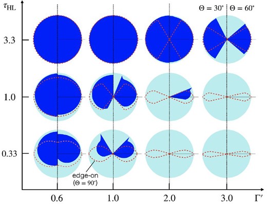
Shapes of accretion cross-section for various Γ′ and τ_HL. The red dotted line indicates the accretion radius for the edge-on model (Θ = 90°). The radius of the light blue circle represents the Hoyle–Lyttleton radii. The blue area is an accretion cross-section with Θ = 30° (left half) and Θ = 60° (right half). (Color online)

Open in new tabDownload slide

As shown in figure 3, the accretion cross-section is larger in the upper left-hand part of the figure for all cases. This is because the smaller Γ′ is, and the larger τ_HL is, the weaker the radiation force which works to prevent the gas accretion. We find that, as it moves to the lower right-hand side, accretion becomes more difficult via the strong radiation force. For (Γ′, τ_HL) = (2.0, 0.33), (3.0, 1.0), and (3.0, 0.33), the accretion disappears for Θ = 30° and for 60° via the strong radiation force. We also find that the most difficult area to accrete is around ϕ = 0° and 180°. For instance, in the case of Θ = 60°, the accretion cross-section is broadened in the ϕ = 90° direction, while the accretion radius is very small or zero around ϕ = 0 and 180° for (Γ′, τ_HL) = (1.0, 0.33), (1.0, 1.0), (2.0, 1.0), and (3.0, 3.3). This is because the radiation flux is large in the direction of the rotation axis of the disk. To the contrary, around ϕ = 90°, which is closer to the disk plane, the radiation force is weaker, so accretion is easier. Also, we find that the accretion cross-section for Θ = 30° and Θ = 60° is not symmetrical to the plane of ϕ = 90° in figure 3 (see appendix 3 for a detailed reason). In particular, for the edge-on model (Θ = 90°), the plane with ϕ = 90° aligns with the disk plane, and thus the radiation flux is zero. Therefore, it is possible to accrete regardless of how large Γ′ becomes, and the horizontally extended accretion cross-section does not disappear in the lower right-hand region of the figure.

3.3 Accretion rate

The resulting mass accretion rate for τ_HL = 0 (optically thin limit, figure 4a), 0.33 (figure 4b), 1.0 (figure 4c), and 3.3 (figure 4d) is presented in figure 4 as a function of Γ′. The purple solid line represents the isotropic model, the green one represents Θ = 0° (pole-on model), the blue one is for Θ = 30°, the yellow one is for Θ = 60°, and the red one represents Θ = 90° (edge-on model).

Fig. 4.

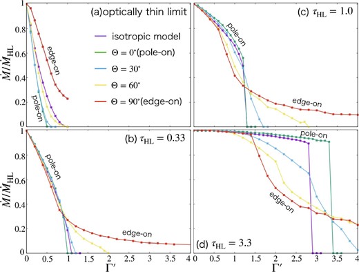
Accretion rate normalized by Hoyle–Lyttleton one as a function of Γ′ for the cases of τ_HL = 0 (optically thin limit, a), τ_HL = 0.33 (b), τ_HL = 1.0 (c), and τ_HL = 3.3 (d). Results for Θ = 0°, 30, 60, and 90 are shown by green, blue, yellow, and red lines, respectively. The purple line is for the isotropic model. (Color online)

Open in new tabDownload slide

In the optically thin limit, the mass accretion rate decreases as an increase of Γ′ (see figure 4a). The accretion rate in the pole-on model is the smallest of all models. This is because the rotation axis of the disk in the pole-on model is aligned with the z-axis, and the radiation force effectively acts on the gas flowing in from the z-direction. For Γ′ > 0.5, the radiation force exceeds the gravity except in the region of z ∼ 0 and the accretion rate becomes zero. The radiation force in the region of z ≫ 0 becomes weaker as Θ approaches 90°, hence the accretion rate in the edge-on model is larger than that in other cases. It should be noted that the mass accretion rate in the edge-on model is not zero even if Γ′ is unity, since the accretion through the vicinity of the disk plane (ϕ = 90°) is not prohibited (see appendix  1). Our results for the pole-on and edge-on models are consistent with those of Fukue and Ioroi (1999).

We can see in figures 4b–4d that the accretion rate increases as τ_HL increases. This is because the attenuation via the dust absorption weakens the radiation force. This figure reveals that the accretion is possible in a super-Eddington regime (Γ′ > 1) not only for the edge-on model but also for all models for τ_HL ≳ 1. Moreover, the dependence of the accretion rate on Θ also changes at the regime of τ_HL ≳ 1. Although the accretion rate increases with increasing Θ for an optically thin limit as shown above, such a trend is reversed as τ_HL increases. Indeed, at the regime of Γ′ ≲ 1.0 (figure 4b), the accretion rate is approximately equal for all models when τ_HL = 0.33 and increases as an increase of Θ in the case of τ_HL = 1.0 (figure 4c). This trend becomes more evident for τ_HL = 3.3. Figure 4d shows that the accretion rate tends to be larger as Θ is smaller except in the range of Γ′ ≳ 3.0.

In the case of large optical thickness (τ_HL = 1.0, 3.3), the accretion rate for the pole-on model exceeds that for the isotropic model, as we have mentioned subsection 3.1. The reason why the accretion rate suddenly decreases to zero is due to the merging of many streamlines (see appendix  1). In addition, even when Γ′ is extremely large, the accretion rate of the edge-on model does not become zero. This is because the radiation force never exceeds the gravity around the disk plane (see appendix  1).

4 Discussion

4.1 Canonical Eddington ratio

Figure 5 shows |$\Gamma ^{\prime }_{\rm {can}}$| as a function of |$\dot{m}_{\rm {dg}}$|⁠. We find that |$\Gamma ^{\prime }_{\rm can}$| increases with an increase of |$\dot{m}_{\rm dg}$| and is almost constant in the region of |$\dot{m}_{\rm dg} \gtrsim 10$| for the isotropic and pole-on models. The maximum values of |$\Gamma ^{\prime }_{\rm can}$| in figure 5 correspond to the upper limits of Γ′ shown in figure 4. This is because there is no canonical Eddington ratio that exceeds the upper limit, since the radiation force prevents the gas accretion. For instance, the maximum value of |$\Gamma ^{\prime }_{\rm can}$| in the pole-on model is 3.4, which is consistent with the upper limit of Γ′ in figure 4d.

Fig. 5.

Canonical Eddington ratio, |$\Gamma_{\rm can}$|⁠, as a function of |$m\,_{\rm dg}[=\eta c \tau_{\rm HL}/(2v_{\infty})]$|⁠. The purple line is for the isotropic model, the green line is for the pole-on model (Θ = 0°), and the red line is for the edge-on model (Θ = 90°). The thick solid, dot–dashed, and dashed lines indicate τ_HL = 3.3, 1.0, and 0.33. The result for the optically thin limit is shown by the thin solid line. (Color online)

Open in new tabDownload slide

On the other hand, in the edge-on model, there is no upper limit for Γ′ (see figure 4). Hence, |$\Gamma ^{\prime }_{\rm can}$| increases as |$\dot{m}_{\rm dg}$| increases. This is because, even though the disk luminosity is large, the gas can accrete through the region near the disk plane, ϕ = 90° (see figure 3).

4.2 Evolution of luminosity

In this section, we first discuss the evolution of a BH with an accretion disk as it moves through a high-density region. If the initial luminosity of the accretion disk is different from the canonical luminosity, |$\kappa _{\rm dg}\Gamma ^{\prime }_{\rm can} L_{\rm Edd}/\kappa _{\rm es}$|⁠, the luminosity gets close to the canonical one and should become the same value finally. This final state corresponds to the fact that the accretion rate of the disk on to a BH becomes consistent with that of the Hoyle–Lyttleton mechanism which takes into account the effect of radiation (i.e., the accretion rate from a larger scale to the disk).

Here we note that Θ also changes on the timescale of t_vis. The direction of the angular momentum of the gas passing through the accretion cross-section, v_∞r_∞, is perpendicular to the z-axis. Therefore, the rotation axis of the accretion disk formed by the accretion gas via the Hoyle–Lyttleton mechanism which takes into account the effect of radiation is also perpendicular to the z-axis. Edge-on accretion (Θ = 90°) would be realized after t_vis, and the disk luminosity is thought to be the canonical luminosity for Θ = 90°. For example, in the case of M = 500 M_⊙, v_∞ = 100 km s⁻¹, and n_∞ = 10⁵ cm⁻³, we have τ_HL ∼ 0.33 and |$\dot{m}_{\rm {dg}}\sim 50$|⁠. The canonical Eddington ratio is |$\Gamma ^{\prime }_{\rm {can}}\sim 3.4$|⁠. Since the disk luminosity is estimated to be L ∼ 10³⁸(M/500 M_⊙)[(κ_dg/κ_es)/1900] erg s⁻¹, and since the ultraviolet/optical photons emitted from the disk are effectively absorbed and infrared photons are re-emitted, the intermediate-mass BHs moving in high-density gas can be identified as bright sources in the infrared band. Also, the X-ray and radio emission of the disk, which transmit through the dusty gas, would be observed. The detailed spectra should be obtained by the multi-wavelength radiation transfer calculations.

This relation implies that the region where the dust is sublimated is negligibly small and our treatment in this paper, which does not consider the effect of sublimation of the dust, is reasonable.

4.3 Future work

By taking account of the dilution of the radiation via the dust absorption, we study the steady structure around moving BHs surrounded by luminous accretion disks. Although the hydrodynamic effects are neglected in the present work, they may play an important role; one of them is the shock wave. A bow shock is thought to be formed if the speed of the moving BH, which corresponds to the velocity of the gas flow (v_∞) in the BH rest frame, is greater than the sound speed. Indeed, the occurrence of a bow shock was reported by the hydrodynamics simulations (Hunt 1971, 1979; Shima et al. 1985; Ruffert & Arnett 1994). Our results also show that the streamlines are bending and merging. Thus shock waves can be generated by the collision of the gas flows. The velocity as well as the density of the flow changes at the shock surface, which might cause the pressure gradient force to become negligible. For instance, the motion of the gas in the ϕ-direction might be induced, although the gas moves in a ϕ-constant plane in the present model. The change in the density distribution causes the change in the radiation field; the gas flow should also then change. In order to reveal the structure of the flow by taking account of the shock, we need to perform multidimensional radiation hydrodynamics simulations. On the other hand, the accretion rate may increase with the occurrence of shock waves. This is because the release of thermal energy via the emitting photons reduces the total energy of the gas, making it more likely to accrete than in the absence of the shock. Also, if the dust is destroyed, the radiative force will be ineffective and the gas will accrete more easily. In order to understand the dust destruction process, it is necessary to study the structure of the shock wave in detail. This requires radiation hydrodynamics simulations, which is an important future work.

In the present paper, although we consider the radiation from the accretion disk around the BH, the jets and disk winds might be launched from the disk (Li et al. 2020). Such outflows also change the structure of the flow around the moving BHs through the collision between the out-flowing matter and the interstellar gas. Research into the effects of the outflows are left as an important future work. In addition, although we focus on the steady structures in this work, time variations might occur. As the disk luminosity (accretion rate) increases, the enhanced radiation force works to reduce the accretion rate. The disk luminosity then decreases via the reduction of the accretion rate, leading to weakening of the radiative force and increasing the accretion rate. Thus, the increase and decrease in the disk luminosity (accretion rate) are repeated. The time variation of the luminosity might cause the time-dependent outflows. In order to investigate Bondi–Hoyle–Lyttleton accretion including the effects mentioned above, we plan to perform multi-dimensional radiation hydrodynamics simulations.

In the present work, we consider a situation in which the absorption coefficient of the dust is larger than the electron scattering opacity. The absorption coefficient of dusty gas depends on the dust-to-gas mass ratio, which is thought to relate to the star formation history. The dust-to-gas mass ratio in our galaxy is estimated to be about 0.01, but it would be much larger in quasars or starburst galaxies (Solomon et al. 1997; Watson et al. 2015). In contrast, it is predicted to be extremely small in the very early universe (Inoue et al. 2016). In addition, the absorption coefficient of dusty gas also depends on α, which is determined by the size distribution and chemical composition of the dust grain (Draine & Lee 1984), as well as on the spectrum of the disk emission. The value of α tends to be larger if the disk shines mainly in the ultraviolet/optical band. In contrast, α becomes small if the radiation is dominant in the radio wave or X-ray band. In the case of the standard disk around the stellar-mass BHs/intermediate-mass BHs, as the BH mass is smaller and the Eddington ratio is larger, the temperature of the disk is known to increase and the X-ray emission is enhanced. Meanwhile, the radiatively inefficient accretion flow, which appears in the regime where the accretion rate is very small (≪L_E/c²), is thought to emit photons mainly at the radio band. The study of the accretion disks that takes account of spectra is also left as an important future work. Moreover, the detailed calculations of observable spectra, consisting of penetrating intrinsic radiation from the disk and the IR photons from the dust, would be important for comparison with observational data. We will investigate the above issues in future work.

5 Conclusions

In this study, we have investigated the steady structure of Hoyle–Lyttleton accretion of dusty gas, assuming that a BH with an accretion disk moves in dense gas. For this purpose, we solve the equation of motion which incorporates the gravity of the central object and the radiation force due to dust absorption, by coupling with the continuity equation and attenuation of the radiation. Here, the scattering process of dust is assumed to be negligibly small.

We find that the gas accretion is possible even when the luminosity is larger than the Eddington luminosity for the dusty gas if the flow is so optically thick that radiation is sufficiently weakened by the dust absorption. For example, in the case of τ_HL = 3.3 and Θ = 0 (the pole-on model), the accretion rate is |$92\%$| of the Hoyle–Lyttleton one even at Γ′ = 3.0. Also, in the edge-on model (Θ = 90°), the gas accretes at a rate of |$32\%$| of the Hoyle–Lyttleton rate. Note that in the regime of Γ′, where gas accretion is possible for all models, the accretion rate tends to be greater as Θ is smaller for the case of τ_HL ≳ 1.0. This is the opposite trend to that of the optically thin case. As mention in appendix  1, this is due to the effects of the optical thickness and the anisotropic radiation field of the disk.

If the optical depth is not sufficient or if the luminosity is extremely large, the radiation force is not sufficiently weakened so that the accretion rate is reduced or the gas accretion becomes impossible. This is confirmed in that the accretion rate for both (Γ′, τ_HL) = (3.0, 1.0) and (Γ′, τ_HL) = (3.4, 3.3) is smaller than that for (Γ′, τ_HL) = (3.0, 3.3). For (Γ′, τ_HL) = (3.0, 1.0), the accretion rate is zero in the case of Θ = 0° and is |$13\%$| of the Hoyle–Lyttleton one in the case of Θ = 90°. For (Γ′, τ_HL) = (3.4, 3.3), the accretion rate is zero when Θ = 0° and is |$30\%$| of the Hoyle–Lyttleton one when Θ = 90°. These values are smaller than those for (Γ′, τ_HL) = (3.0, 3.3).

Although the accretion rate rapidly goes to zero as Γ′ becomes large for the case of Θ = 0°, the decrease in the accretion rate due to the increase in Γ′ becomes moderate as Θ approaches 90°. This is because, even if the luminosity of the disk is very large, the radiative flux in the direction of the disk plane is small, so the radiation force is less effective in preventing accretion of the gas passing around the disk plane. Hence, a sharp decrease does not appear for models with Θ ≳ 60°. In particular, in the case of Θ = 90°, the accretion rate does not decrease to zero even if Γ′ is extremely large.

Furthermore, we obtain the canonical Eddington ratio, where the mass accretion rate and the disk luminosity become consistent (the accretion rate by the Hoyle–Lyttleton mechanism which takes into account the effect of radiation and the disk luminosity satisfy the relation of |$L=\eta \dot{M} c^2$|⁠), using fitting functions for the numerical results. The Eddington ratio of a BH accretion disk moving in dense dusty gas is likely to evolve into a canonical Eddington ratio. The rotation axis of the disk also changes and would be Θ = 90° at that time. For instance, if a BH with 500 M_⊙ moves in a dense dusty gas with 10⁵ cm⁻³ at a speed of 100 km s⁻¹, the canonical Eddington ratio is ∼3.4. Since the disk luminosity is L ∼ 10³⁸(M/500 M_⊙)[(κ_dg/κ_es)/1900] erg s⁻¹, intermediate-mass BHs moving in dense dusty gas would be observed as bright sources in the infrared band. However, there is some uncertainty about the absorption coefficient of the dust, which is thought to depend on the dust-to-gas mass ratio, the composition and the size distribution of the dust grain, and the spectrum of the accretion disk.

Acknowledgements

This research used computational resources in Center for Computational Sciences, University of Tsukuba. This work was supported by JSPS KAKENHI Grant Numbers JP18K03710 (KO), 17H04827, 20H04724 (HY), National Astronomical Observatory of Japan (NAOJ) ALMA Scietific Research Grant Number 2019-11A (HY) and by MEXT as “Program for Promoting Researches on the Supercomputer Fugaku” (Toward a unified view of the universe: from large scale structures to planets, KO) and by Joint Institute for Computational Fundamental Science (JICFuS, KO).

Appendix 1 Effects of disk emission

Figure 6a shows the streamlines closest to the z-axis in the case of Γ′ = 3.0 for the pole-on model (purple) and for the isotropic model (green). These lines are the same as those shown in figures 2b and 2d. We also plot the z-component of the velocity (figure 6b), the radiation force (figure 6c), and the optical depth (figure 6d) on the streamlines. Figure 3e indicates the mass transported along the streamline per unit time (mass transport rate). The mass transport rate increases by the merging of the streamlines.

Fig. 6.

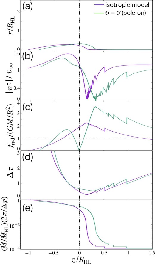
Streamlines closest to the z-axis (a) for the case of τ_HL = 3.3 and Γ′ = 3.0. The purple and green lines are for the isotropic model and for the pole-on model. We also plot the z-component of the velocity (b), the ratio of radiation force to gravity (c), and the optical depth (d) on the streamlines. The mass transport rate is shown in panel (e). (Color online)

Open in new tabDownload slide

As we have mentioned in subsection 3.1, the streamlines are approximately parallel to the z-axis at z/R_HL ≫ 1.0 for both models (figure 6a). The streamlines bend significantly in the region where z/R_HL ≲ 0.3. The gas leaves the z-axis once, approaches it again, and finally reaches the z-axis. In figure 6b, we can see that |−v^z| substantially decreases in the region of 0.25 ≲ z ≲ 1.0 for both models. In this region, the radiation force is stronger than the gravity (see figure 6c), leading to a slow-down.

Here we note that a jagged structure, as shown in figures 6b–6e, is caused by the merging of the streamlines. In our method, when two streamlines merge into one, the mass transport rate and the velocity change based on the mass conservation law and the momentum conservation law (see subsection 2.3). The mass transport rate becomes the sum of the mass transport rate of the two streamlines. Thus, the velocity discontinuously changes, producing the jagged structure in figure 6b. By repeating the merger, the mass transport rate increases from right to left in figure 6e. Furthermore, by the change of the velocity and the mass transport rate, the jagged structure appears in figures 6c and 6d.

As shown in figure 6b, the velocity (|−v^z|) of the isotropic model increases in the region of 0 ≤ z ≤ 0.15, even though the radiation force is stronger than the gravity. This is caused by the the merging of the streamlines. The streamlines further from the z-axis (streamlines with large i) tend not to be decelerated by the radiation force, since the incident radiation is more attenuated by the dust absorption. Such less-decelerated streamlines merge into the streamline with i = 1 so that the velocity increases. The velocity −v^z/v_∞, which is ∼0.1 at z/R_HL ∼ 0.15, becomes ∼1.0 at around z/R_HL = 0. The increase in the velocity due to merging continues until z/R_HL ∼ −0.2.

Similarly to the isotropic model, the pole-on model also shows an increase of velocity due to merging. The velocity |−v^z|/v_∞, which is ∼0 at z/R_HL ∼ 0.3, becomes ∼1.4 at around z/R_HL = −0.3. However, the effect of the unisotropic radiation appears in the case of the pole-on model. The radiation force is less than the gravity around z = 0. The reason is that the plane of z = 0 coincides with the disk plane. Thus, the streamline of the pole-on model begins to approach the z-axis before that of the isotropic model. As a result, the upper and lower positions of the streamlines are switched at around z ∼ −0.2 (figure 6a).

It is found that the radiation force is less than gravity in the region of z ≲ −0.5 (pole-on model) and z ≲ −0.3 (isotopic model). The reduction of the radiation force is induced by the attenuation of the radiation. In the above regions, the optical depth of the streamline is much larger than unity (figure 6d), since many streamlines merge into the one streamline, and since the flow is concentrated in the z-axis (the streamlines approach the z-axis). Hence, the radiation force cannot increase the velocity, and the gas reaches the z-axis with a slight deceleration. Finally, the gas accretes on to the center for the case of the pole-on model. However, in contrast, the streamline for the isotropic model does not satisfy the accretion condition since the reach point is slightly further from the center in comparison with the pole-on model.

To sum up, (i) a strong radiation force initially leads to the deceleration and merging of the streamlines, (ii) the streamlines approach the z-axis due to weak radiation force at around z = 0 (the disk plane), and (iii) the radiation force cannot effectively accelerate the gas behind the BH. Therefore, the accretion rate becomes large for the pole-on model. For the case of the isotropic model, (ii) does not occur, so the accretion rate is drastically reduced. In order to achieve a large accretion rate, both the unisotropic radiation fields and the attenuation of the radiation are needed.

Figure 7 shows the accretion radius r_acc normalized by the Hoyle–Lyttleton accretion radius R_acc as a function of Γ′ for the isotropic model and the pole-on model. Here, the accretion radius is r_∞(i) of the outermost streamline, satisfying the accretion condition. The accretion rate is obtained using the accretion radius as |$\dot{M} = \pi r_{\rm acc}^2 \rho _\infty v_\infty$|⁠.

Fig. 7.

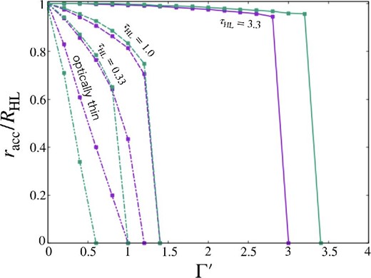
Accretion radius normalized by the Hoyle–Lyttleton one, r_acc/R_HL, as a function of the effective Eddington ratio Γ′. The results for the isotropic and pole-on models are plotted by purple and green lines. The solid, dashed, and dash-dotted lines are for τ_HL = 3.3, 1.0, and 0.33, respectively. The double-dot–dashed lines indicate the cases of the optically thin limit. (Color online)

Open in new tabDownload slide

As shown in figure 7, the accretion radius tends to decrease as Γ′ increases. This is because the strong radiation force works to push the gas and prevent the accretion. However, since the radiation force is weakened by attenuation, accretion is possible even for a super-Eddington regime (Γ′ > 1) for the case of τ_HL = 1.0 and 3.0. The effect of attenuation is more effective for larger τ_HL; the accretion radius is larger for τ_HL = 3.0 than for τ_HL = 1.0. In the optically thin limit, the accretion radius of the isotropic model is larger than that of the pole-on model, since the radiation flux is enhanced at around the rotation axis of the disk (z-axis), effectively pushing the gas coming from the z-direction. However, the difference between the isotropic model and the pole-on model becomes gradually smaller with an increase of τ_HL, and r_acc for the pole-on model exceeds that for the isotropic model in the case of τ_HL ≳ 1.0 (see section 3.1 for detailed reason).

It is found that the accretion radius for τ_HL = 3.3 rapidly decreases to zero at Γ′ ∼ 3.4 for the pole-on model and at Γ′ ∼ 2.8 for the isotropic model. Also, in the case of τ_HL = 1.0, the accretion radius suddenly becomes zero at Γ′ ∼ 1.3 for both models. This can be understood as follows. In the case of large Γ′, the streamlines bend considerably near the center via the strong radiation force, and many streamlines merge into one. The mass transport rate of this single streamline becomes large. Thus the accretion rate varies greatly depending on whether this streamline satisfies the accretion condition or not. For example, we can see that the streamline nearest to the z-axis is responsible for about |$80\%$| of the mass transport rate. If this streamline satisfies the accretion condition, the accretion rate exceeds |$0.8\dot{M}_{\rm HL}$|⁠. In the situation where the accretion condition is not satisfied for this streamline, other streamlines do not satisfy the condition since their reach points are more distant. Thus, the accretion rate becomes zero.

Appendix 2 Asymmetry of accretion cross-section

In figure 3, we find that the accretion cross-section for Θ = 30° and 60° is not symmetrical to the plane of ϕ = 90°. The cross-section for ϕ < 90° is larger than that for ϕ > 90° for the case of (τ_HL, Γ′) = (0.33, 1.0), (1.0, 1.0), and (1.0, 2.0). Such a trend is understood in figure 8, which is the same as figure 2 but for (τ_HL, Γ′) = (0.33, 1.0). The upper and lower panels show the flow structure of ϕ = 63° and ϕ = 117°, respectively. The dotted lines indicate the direction of the disk plane. The region where the radiation force exceeds gravity is larger in figure 2 than in figure 8. This is due to the small optical thickness (τ_HL = 0.33).

Fig. 8.

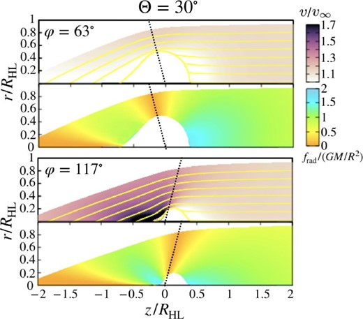
Same as figure 2 but for Θ = 30°, where τ_HL = 0.33 and Γ′ = 1.0 are employed. The upper and lower panels show results on the plane of ϕ = 63° and 117°. The dotted lines indicate the direction of the disk plane. (Color online)

Open in new tabDownload slide

In the case of ϕ = 63° (upper panel), the flow is closest to the rotation axis of the disk in the region of z > 0. In this region, the radiation force, which is much stronger than the gravity, effectively reduces the flow velocity. The streamlines near the z-axis are bent significantly and many streamlines merge at 0 ≲ z/R_HL ≲ 0.5. At the region of z < 0, the radiation force does not exceed the gravity since this region is relatively close to the disk plane (dotted line), and since the flow is very optically thick. Hence, the gas reaches the z-axis while being slowed down by the gravity.

The flow is effectively slowed down even in the case of ϕ = 117° (bottom panel). However, the flow passes through the disk plane (dotted line) at the region of z > 0. Thus, the flow tends to be less decelerated than in the case of ϕ = 63°. Due to the relatively weak radiation force, the bending of streamlines is small and the number of merging streamlines is small. The flow approaches the rotation axis of the disk in the region of z < 0. The strong radiation force, which is stronger than the gravity, accelerates the flow so that the gas reaches the z-axis at a relatively high speed.

As described above, the difference in radiation force leads to the difference in the velocity distribution. The flow velocity of ϕ = 63° is lower than that of ϕ = 117°, so that the accretion condition is more likely to be satisfied in the case of ϕ = 63°. Thus, the accretion cross-section becomes wider for ϕ < 90° than for ϕ > 90°.

References