Angular clustering and host halo properties of [O ii ] emitters at z &gt; 1 in the Subaru HSC survey

Summary of the [O ii] ELG data used in this paper.*

	NB816 (1.178 < z < 1.208)				NB921 (1.453 < z < 1.489)
Field	Area (deg²)	N_g	n_g (h³ Mpc⁻³)	N_sub	Area (deg²)	N_g	n_g (h³ Mpc⁻³)	N_sub
COSMOS	1.37	566	4.48 × 10⁻³	9	5.80	3134	4.30 × 10⁻³	41
DEEP2-3	4.98	2485	5.40 × 10⁻³	35	4.92	2107	3.41 × 10⁻³	35
ELAIS-N1	4.81	2927	6.59 × 10⁻³	34	4.81	3098	5.13 × 10⁻³	34
SXDS+XMM-LSS	5.17	2324	4.86 × 10⁻³	37	1.33	1239	7.44 × 10⁻³	9
Total	16.33	8302	5.50 × 10⁻³	115	16.86	9578	4.53 × 10⁻³	119

	NB816 (1.178 < z < 1.208)				NB921 (1.453 < z < 1.489)
Field	Area (deg²)	N_g	n_g (h³ Mpc⁻³)	N_sub	Area (deg²)	N_g	n_g (h³ Mpc⁻³)	N_sub
COSMOS	1.37	566	4.48 × 10⁻³	9	5.80	3134	4.30 × 10⁻³	41
DEEP2-3	4.98	2485	5.40 × 10⁻³	35	4.92	2107	3.41 × 10⁻³	35
ELAIS-N1	4.81	2927	6.59 × 10⁻³	34	4.81	3098	5.13 × 10⁻³	34
SXDS+XMM-LSS	5.17	2324	4.86 × 10⁻³	37	1.33	1239	7.44 × 10⁻³	9
Total	16.33	8302	5.50 × 10⁻³	115	16.86	9578	4.53 × 10⁻³	119

*

The area value is after masking with bright object masks, N_g is the number of galaxies used in this paper after making the magnitude and flux cuts, n_g is the number densities of the galaxies, and N_sub is the number of sub-regions using jackknife resampling (see subsection 3.2). The last row shows the values for the sum of the four fields.

Table 1.

Summary of the [O ii] ELG data used in this paper.*

	NB816 (1.178 < z < 1.208)				NB921 (1.453 < z < 1.489)
Field	Area (deg²)	N_g	n_g (h³ Mpc⁻³)	N_sub	Area (deg²)	N_g	n_g (h³ Mpc⁻³)	N_sub
COSMOS	1.37	566	4.48 × 10⁻³	9	5.80	3134	4.30 × 10⁻³	41
DEEP2-3	4.98	2485	5.40 × 10⁻³	35	4.92	2107	3.41 × 10⁻³	35
ELAIS-N1	4.81	2927	6.59 × 10⁻³	34	4.81	3098	5.13 × 10⁻³	34
SXDS+XMM-LSS	5.17	2324	4.86 × 10⁻³	37	1.33	1239	7.44 × 10⁻³	9
Total	16.33	8302	5.50 × 10⁻³	115	16.86	9578	4.53 × 10⁻³	119

	NB816 (1.178 < z < 1.208)				NB921 (1.453 < z < 1.489)
Field	Area (deg²)	N_g	n_g (h³ Mpc⁻³)	N_sub	Area (deg²)	N_g	n_g (h³ Mpc⁻³)	N_sub
COSMOS	1.37	566	4.48 × 10⁻³	9	5.80	3134	4.30 × 10⁻³	41
DEEP2-3	4.98	2485	5.40 × 10⁻³	35	4.92	2107	3.41 × 10⁻³	35
ELAIS-N1	4.81	2927	6.59 × 10⁻³	34	4.81	3098	5.13 × 10⁻³	34
SXDS+XMM-LSS	5.17	2324	4.86 × 10⁻³	37	1.33	1239	7.44 × 10⁻³	9
Total	16.33	8302	5.50 × 10⁻³	115	16.86	9578	4.53 × 10⁻³	119

*

The area value is after masking with bright object masks, N_g is the number of galaxies used in this paper after making the magnitude and flux cuts, n_g is the number densities of the galaxies, and N_sub is the number of sub-regions using jackknife resampling (see subsection 3.2). The last row shows the values for the sum of the four fields.

The survey area in the D layer, where the NB data are available, consists of four separate fields: E-COSMOS, DEEP2-3, ELAIS-N1, and XMM-LSS. Furthermore, each of the E-COSMOS and XMM-LSS fields encompasses the UD layer covered by a single pointing of HSC, named UD-COSMOS and SXDS, respectively. Since UD-COSMOS and E-COSMOS are jointly processed, we call the combination the COSMOS field.

Complete descriptions of the [O ii] emitter sample used in this study are provided in Hayashi et al. (2018, 2020). While we briefly summarize our sample in the following, we refer the reader to these papers for more details.

The ELGs are selected using the NB data together with data from the five BB filters. [O ii] emitters are observed by NB816 and NB921 filters in two narrow redshift ranges, 1.178 < z < 1.208 and 1.453 < z < 1.489, respectively. To identify the [O ii] emitters, we use spectroscopic redshifts if available and photometric redshifts otherwise. If a galaxy has a spectroscopic redshift outside the above ranges, we remove it as a contaminant. When the photometric redshift is used, we have taken into account its uncertainty for the identification of [O ii] emitters. For galaxies not identified with spectroscopic or photometric redshifts, we use color–color diagrams to distinguish [O ii] emitters from other possibilities. Galaxies selected as NB [O ii] emitters are expected to be star-forming galaxies (Ly et al. 2012; Hayashi et al. 2013). Thus, our sample is limited by star formation rate (SFR). While our [O ii] emission lines are affected by dust extinction, the majority of typical star-forming galaxies are properly selected because the cosmic SFR density in our catalogs is consistent with previous studies (Hayashi et al. 2020).

We make magnitude and flux cuts on our data: the model magnitude¹ m ≤ 23.5 and the estimated line flux ≥3 × 10⁻¹⁷ erg s⁻¹ cm⁻². We refer the reader to Hayashi et al. (2020) for details of the line flux estimation. The limiting magnitude of the NB filters is much deeper than 23.5 [mag] so that fainter [O ii] emitters have been included in our sample, and accordingly [O ii] emitters which have a line flux of (1–2) × 10⁻¹⁷ erg s⁻¹ cm⁻² have been selected. However, we have made such conservative magnitude and flux cuts to assure the completeness of the sample. With these ranges, the number density indeed increases monotonically with decreasing flux or increasing magnitude (see Hayashi et al. 2018, 2020) and the mean completeness of our [O ii] sample becomes 0.974 for NB816 and 0.956 for NB921. The numbers of [O ii] emitters are then reduced to 8302 and 9578 for the NB816 and NB921 data, respectively. See table 1 for the sample numbers for each field. The line flux cut corresponds to observed line luminosity thresholds of |$L \ge 2.56\times 10^{41} \, \rm {[erg\, s^{-1}]}$| (z = 1.19) and |$L \ge 4.30 \times 10^{41} \, \rm {[erg \, s^{-1}]}$| (z = 1.47). The median luminosity with the 2.5th–97.5th percentiles is |$\bar{L} = 4.49^{+12.67}_{-1.82} \times 10^{41} \, \rm {[erg \, s^{-1}]}$| at z = 1.19 and |$\bar{L} = 7.88^{+16.95}_{-3.35} \times 10^{41} \, \rm {[erg \, s^{-1}]}$| at z = 1.47. Stellar masses for the [O ii] emitters are estimated by spectral energy distribution fit with five HSC BB data in Hayashi et al. (2020). The median stellar mass of our [O ii] emitter sample with the 2.5th–97.5th percentiles is |$\bar{M}_* = 8.58^{+132.54}_{-7.13}\times 10^{9}\, {M}_{\odot }$| at z = 1.19 and |$\bar{M}_* = 1.72^{+12.40}_{-1.41}\times 10^{10}\, {M}_{\odot }$| at z = 1.47.

Not all the galaxies in the catalog are real [O ii] emitters; some are fake lines due to noise and some others are real emission lines but not [O ii] emitters. The contamination rate is investigated by applying photo-z and color selections to galaxies confirmed with spectroscopic redshifts. The fraction of such non-[O ii] emitters has been significantly reduced in the current sample compared to that in the PDR1 catalog because (i) the method of selecting emission line galaxies has been improved from using the cmodel magnitude to the fixed aperture magnitude (Hayashi et al. 2020), and (ii) the pipeline used for the data processing, hscPipe, has been upgraded in PDR2 (Bosch et al. 2018; Aihara et al. 2019). The analysis by Hayashi et al. (2020) estimated the fraction of non-[O ii] emitters in our sample at less than |$10\%$| for most cases and ∼20% at most, by applying photometric redshift and color selections to galaxies confirmed with spectroscopic redshifts. This contaminant fraction can be further reduced by a machine-learning-based technique for photometric redshift estimates (see, e.g., Hsieh & Yee 2014). However, since the current contaminant fraction is low enough for our analysis, we do not include this process. The angular distribution of the [O ii] emitters is shown in figure 1. Table 1 summarizes the properties of the data.

Angular distribution of [O ii] emitters at z = 1.19 (top) and z = 1.47 (bottom) with line flux greater than 3 × 10−17 erg s−1 cm−2 and magnitude brighter than 23.5 mag in the NB816 and NB921 filters, respectively, for the four individual fields. The large empty areas where no galaxy is found are mostly the regions masked for bright objects. See figure 4 of Hayashi et al. (2020) for details of the mask information. (Color online)

Fig. 1.

Angular distribution of [O ii] emitters at z = 1.19 (top) and z = 1.47 (bottom) with line flux greater than 3 × 10⁻¹⁷ erg s⁻¹ cm⁻² and magnitude brighter than 23.5 mag in the NB816 and NB921 filters, respectively, for the four individual fields. The large empty areas where no galaxy is found are mostly the regions masked for bright objects. See figure 4 of Hayashi et al. (2020) for details of the mask information. (Color online)

2.3 Random catalog

HSC-SSP PDR2 provides us with a catalog of random points across the survey area as one of the value-added products (see subsection 5.4 of Aihara et al. 2019). The number density of the random points is 100 arcmin⁻². We apply the same basic flags as those for the emission line galaxies except for the flags related to source detection (i.e., merge_peak, sdssshape_flag, cmodel, and psfflux) to select the random points (see, sub-subsection 2.1.1 of Hayashi et al. 2020). We also apply the same bright star masks used for the selection of the emission line galaxies to the random points (see Hayashi et al. 2020 for the details of the masks; sub-subsection 6.6.2 of Aihara et al. 2019; Coupon et al. 2018). Consequently, the random points used in this study are distributed over regions identical to where the emission line galaxies are surveyed.

3 Angular correlation function

In this paper we analyze the spatial distribution of [O ii] emitters using the angular correlation function. This is related to the spatial correlation function in three dimensions through (Peebles 1973, 1980)

$$\begin{equation} w(\theta ) = \int dx_1 p(x_1) \int dx_2 p(x_2) \xi (r), \end{equation}$$

(1)

where r is the three-dimensional separation between two galaxies, |$r = (x_1^2+x_2^2-2x_1x_2\cos {\theta })^{1/2}$|⁠, x_i = x(z_i) is the comoving distance to a galaxy at redshift z_i, and p(x) is the radial selection function normalized as |$\int ^\infty _0dxp(x)=1$|⁠.

3.1 Correlation function estimation

We first measure the angular correlation function of [O ii] emitters at z = 1.19 and z = 1.47 from the four fields COSMOS, DEEP2-3, ELAIS-N1, and SXDS + XMM-LSS. We then combine the four correlation functions at each redshift for the statistical analysis.

We adopt the Landy–Szalay estimator (Landy & Szalay 1993) to measure the angular correlation function,

$$\begin{equation} \hat{w}_k(\theta )=\frac{DD_k-2DR_k-RR_k}{RR_k}, \end{equation}$$

(2)

where DD_k, RR_k, and DR_k are respectively the normalized counts of data–data, random–random, and data–random pairs at a given angular separation θ. The random catalogs contain large numbers of points which are more than 600 times as dense as our [O ii] emitter catalogs to ensure that the shot noise due to the finite random points is negligible. The subscript k denotes the kth field (1 ≤ k ≤ 4), and the hat means an estimated quantity which can be different from the true one [see equation (6) below]. To combine the correlation function measurements from the four fields, we weight each measurement by a function W_k,

$$\begin{equation} 1+\hat{w}(\theta ) = \frac{\sum _{k=1}^4W_k^2(\theta ) \left[ 1+\hat{w}_k(\theta )\right] }{\sum _{k=1}^4W_k^2(\theta )}. \end{equation}$$

(3)

Thus, the combined correlation function is expressed as

$$\begin{equation} \hat{w}(\theta ) = \frac{\sum _{k=1}^4W_k^2(\theta ) \hat{w}_k(\theta )}{\sum _{k=1}^4W_k^2(\theta )}. \end{equation}$$

(4)

We adopt the inverse-variance weighting, |$W_k(\theta )=\sigma _k^{-1}(\theta )$|⁠, where |$\sigma _k^2(\theta )$| is the diagonal component of the covariance matrix in the kth field (see next subsection).

The correlation function measured above is underestimated by a constant due to the finite survey area. The effect is known as the integral constraint (Peebles & Groth 1976) and calculated as

$$\begin{equation} w_\Omega = \frac{1}{\Omega }\int _\Omega d\Omega _1d\Omega _2w(\theta ), \end{equation}$$

(5)

where the integral is performed over the solid angle of the survey, Ω. The integral constraint is calculated by a given model of the correlation function w(θ; Θ), where Θ is a set of model parameters (see sections 4 and 5). Note also that the clustering amplitude is further reduced compared to the true clustering of [O ii] emitters due to the contamination of non-[O ii] emitters and noise lines. As seen in section 4, we assume that the correlation of non-[O ii] emitters is negligible. Then the estimated correlation function is related to the true correlation function w as

$$\begin{equation} \hat{w}(\theta ) = (1-f_{\rm fake})^2 [w(\theta ) - w_\Omega )], \end{equation}$$

(6)

where f_fake is the fraction of non-[O ii] emitters in our sample, 0.1 ≲ f_fake ≲ 0.2 (see subsection 2.2).

The measured correlation function combined over the four fields, |$\hat{w}$|⁠, is shown as the red points in the upper and lower panels of figure 2 for z = 1.19 and z = 1.47, respectively. The correlation function becomes negative at scales θ ∼ 1° (r ∼ 50 h⁻¹ Mpc), due to the integral constraint |$w_\Omega$|⁠. For the model parameter fitting below, this effect is properly taken into account. In this figure we show various lines which are the predictions based on the power-law model and the linearly biased dark matter model. We discuss these in detail in section 4. The measurements of the angular correlation functions for individual fields are presented for a consistency check in appendix 1.

$Angular correlation functions of [O ii] emitters measured from all four fields at z = 1.19 (top) and z = 1.47 (bottom). Note that the vertical axis mixes logarithmic and linear scalings. The red points are measurements without the integral constraint correction, $\hat{w}$. The error bars are estimated from jackknife resampling. The blue solid curve is the best-fitting model of the power-law model, $(1-f_{\rm fake})^2[w(\theta ;A_w,\beta )-w_\Omega (A_w,\beta )]$, with (Aw, β, ffake) = (1.10, 0.534, 0.140) for z = 1.19 and (1.17,0.538,0.139) for z = 1.47. The data enclosed by the two blue vertical lines are used for this analysis. The red solid curve is the best-fitting model of the linearly biased dark matter model, $(1-f_{\rm fake})^2[b^2w_{\rm m}(\theta )-w_\Omega (b)[$, with (b, ffake) = (1.60, 0.140) for z = 1.19 and (2.08,0.140) for z = 1.47 when the data enclosed by the two red vertical lines are used. The red dashed curve is the same model but without subtracting the integral constraint denoted by IC in the legend, (1 − ffake)2b2wm(θ). The non-linear dark matter correlation function, wm(θ), is shown by the red dashed curve as a reference. (Color online)$

Fig. 2.

Angular correlation functions of [O ii] emitters measured from all four fields at z = 1.19 (top) and z = 1.47 (bottom). Note that the vertical axis mixes logarithmic and linear scalings. The red points are measurements without the integral constraint correction, |$\hat{w}$|⁠. The error bars are estimated from jackknife resampling. The blue solid curve is the best-fitting model of the power-law model, |$(1-f_{\rm fake})^2[w(\theta ;A_w,\beta )-w_\Omega (A_w,\beta )]$|⁠, with (A_w, β, f_fake) = (1.10, 0.534, 0.140) for z = 1.19 and (1.17,0.538,0.139) for z = 1.47. The data enclosed by the two blue vertical lines are used for this analysis. The red solid curve is the best-fitting model of the linearly biased dark matter model, |$(1-f_{\rm fake})^2[b^2w_{\rm m}(\theta )-w_\Omega (b)[$|⁠, with (b, f_fake) = (1.60, 0.140) for z = 1.19 and (2.08,0.140) for z = 1.47 when the data enclosed by the two red vertical lines are used. The red dashed curve is the same model but without subtracting the integral constraint denoted by IC in the legend, (1 − f_fake)²b²w_m(θ). The non-linear dark matter correlation function, w_m(θ), is shown by the red dashed curve as a reference. (Color online)

3.2 Covariance matrix

We use the jackknife resampling technique to estimate the covariance error matrix (see, e.g., Lupton 1993). The covariance of the angular correlation function for the kth field, |$C_{k,ij}\equiv C[\hat{w}_k(\theta _i), \hat{w}_k(\theta _j)]$|⁠, is then estimated as

$$\begin{eqnarray} C_{k,ij} &=& \frac{N_{\rm sub}-1}{N_{\rm sub}} \nonumber \\ && \times \sum ^{N_{\rm sub}}_{\ell =1} \left[\hat{w}^\ell _k(\theta _i)-\bar{\hat{w}}_k(\theta _i)\right] \left[\hat{w}^\ell _k(\theta _j)-\bar{\hat{w}}_k(\theta _j)\right], \end{eqnarray}$$

(7)

where |$\hat{w}^\ell _k(\theta _i)$| is the correlation function in the ith angular bin in the ℓth jackknifed realization, N_sub is the number of realizations in the kth field, and |$\bar{\hat{w}}_k(\theta _i)=N_{\rm sub}^{-1}\sum ^{N_{\rm sub}}_{\ell =1}\hat{w}^\ell _k(\theta _i)$|⁠. The values of N_sub for each field are shown in table 1. In total, we use 115 and 119 jackknifed realizations for the z = 1.19 and 1.47 data, respectively. We use the k-means algorithm² to divide our survey regions into subregions with the same angular areas. Each subsample includes a region continuous on the sky, 0|${_{.}^{\circ}}$|38 on a side, which corresponds to a comoving size of 17 h⁻¹ Mpc at z = 1.19 and 20 h⁻¹ Mpc at z = 1.47. Just like equation (4), the covariance matrices from the four fields can be combined to C_ij ≡ C[w(θ_i), w(θ_j)] as

$$\begin{equation} C_{ij} = \frac{\sum _{k=1}^4 W_k^2(\theta _i)W_k^2(\theta _j)C_{k,ij}}{\sum _{k=1}^4W_k^2(\theta _i)\sum _{k=1}^4W_k^2(\theta _j)} . \end{equation}$$

(8)

The square roots of the diagonal components of the covariance matrix, |$C_{ii}^{1/2}$|⁠, are shown as the error bars in figure 2.

4 Results

4.1 Setup

In this section we consider two simple models for the angular correlation function, the power-law and linearly biased dark matter models in subsections 4.2 and 4.3, to model the clustering amplitude of [O ii] emitters. The HOD modeling is performed in section 5.

We adopt the small-angle approximation, known as the Limber’s approximation (Limber 1954; Peebles 1980). With this, the relation between the angular and spatial correlation functions given by equation (1) can be simplified to

$$\begin{equation} w(\theta ) = 2\int ^\infty _0 dx p^2(x) \int ^\infty _0 dh \xi \left( r=\sqrt{x^2\theta ^2+h^2} \right), \end{equation}$$

(9)

where x = (x₁ + x₂)/2 and h = x₂ − x₁. The validity of Limber’s approximation for the angular correlation with large angle separations has been extensively discussed, e.g., by Simon (2007) and Crocce, Cabré, and Gaztañaga (2011). The approximation breaks down at large scales when the width of the redshift distribution, z_min ≤ z ≤ z_max, is too narrow. The width of our NB filters is Δx ≡ x_max − x_min ≃ 50 h⁻¹ Mpc, where x_min = x(z_min) and x_max = x(z_max), and our analysis focuses on the angular scales of θ < 1°. We can thus safely rely on this approximation.

Although determination of the true radial selection function is not straightforward, it is known to have a form similar to the transmission curve to some extent (see, e.g., figure 3 of Hayashi et al. 2015). However, the width Δx ≃ 50 h⁻¹ Mpc is narrow enough that we can simply assume the radial selection function to be a constant,

$$\begin{eqnarray} p(x)= \left\lbrace \begin{array}{ll}1/\Delta x&\quad {\rm for }\, x_{\rm min} \le x \le x_{\rm max}, \\ 0 &\quad {\rm otherwise}. \end{array} \right. \end{eqnarray}$$

(10)

Using the transmission curves available for the NB filters,³ we test the effect of choices of p(z) on the calculation of the angular correlation functions. We compare the angular correlation function computed using p(z) from the transmission curve with that from the constant p(z) in equation (10). We then find that the correlation functions w(θ) have exactly the same shape, with the amplitude differing by ≤7% for both NB816 and NB921. Thus, the constraints on the parameters for the correlation function are not affected by the choice of p(z); it changes only the normalization, f_fake, by at most |$4\%$|⁠, much smaller than our 1 σ prior on f_fake, ∼40% (see the following paragraphs of this subsection). In the following analysis, we thus adopt the simple constant radial selection function [equation (10)].

Given a model for the correlation function with a set of parameters Θ, w(θ; Θ), the integral constraint [equation (5)] can be estimated as

$$\begin{equation} w_\Omega (\Theta ) = \frac{\sum _i{w(\theta _i;\Theta )RR(\theta _i)}}{\sum _i{RR(\theta _i)}}, \end{equation}$$

(11)

where θ_i is the ith separation bin and the sum is calculated over all the bins. The normalized random–random pair count for the combined field, RR, is computed in the same way as the correlation function in equation (4),

$$\begin{equation} RR(\theta ) = \frac{\sum _{k=1}^4W_k^2(\theta ) RR_k(\theta )}{\sum _{k=1}^4W_k^2(\theta )}. \end{equation}$$

(12)

As discussed in subsection 2.2, not all the lines detected as [O ii] emitters are actually [O ii] lines, but some are other emission lines or just noise. The fraction of fake [O ii] lines is denoted as f_fake. Then, the observed correlation function has contributions not only from the auto-correlation of [O ii] emitters but also from the auto-correlation of fake lines and their cross-correlation, which are suppressed by factors of |$f_{\rm fake}^2$| and 2f_fake(1 − f_fake), respectively; see, e.g., van den Bosch et al. (2013) and Okumura et al. (2015, 2017) for detailed theoretical schemes for the tracer decomposition. The contamination fraction is estimated to be around f_fake ∼ 0.14 by applying photometric redshift and color selections to galaxies confirmed with spectroscopic redshifts (Hayashi et al. 2020). Thus, even though the non-[O ii] emitters have a non-negligible auto-correlation, the (intrinsically small) clustering amplitude is suppressed by 0.14² ∼ 0.02. We can therefore safely assume that the observed correlation is dominated by the auto-correlation of [O ii] emitters (for a similar treatment, see, e.g., Okumura et al. 2016; Kashino et al. 2017).⁴ The amplitude of the correlation function is thus simply scaled by a factor of (1 − f_fake)². We treat f_fake as a free parameter with a prior of f_fake = 0.140 ± 0.060 to cover the uncertainties described in subsection 2.2 within the 1 σ confidence level. We chose this uncertainty to be very conservative and to avoid inducing biased constraints on model parameters by imposing strong (and possibly incorrect) priors. The imposed prior is coincidentally equivalent to that adopted in Kashino et al. (2017).

Finally, once the model with parameters for the correlation function is given as w(θ; Θ), the theoretical prediction to be compared to the observed correlation function, |$\hat{w}$|⁠, is obtained with an additional parameter f_fake through equation (6). To constrain the model parameters, the χ² statistic is calculated for the correlation function, w, as

$$\begin{equation} \chi _w^2 (\Theta )= \sum _{i=1}^{N_{\rm bin}}\sum _{j=1}^{N_{\rm bin}} {\Delta _i C^{-1}_{ij} \Delta _j}, \end{equation}$$

(13)

where N_bin is the number of angular separation bins used in the analysis, |$\Delta _i = \hat{w}_{\rm obs}(\theta _i)-\hat{w}_{\rm th}(\theta _i;\Theta )$| is the difference between the observed correlation function [equation (4)] and the theoretical prediction [equation (6)], with Θ being a set of parameters to be constrained, and |$C^{-1}_{ij}$| is the inverse covariance matrix [equation (8)] multiplied by a correction for the finite realization effect, (N_sub − N_bin − 2)(N_sub − 1)⁻¹ (Hartlap et al. 2007).

In order to perform a maximum likelihood analysis we use the Markov chain Monte Carlo (MCMC) sampler emcee (Foreman-Mackey et al. 2013).

4.2 Power-law constraints

It is known that the shapes of the spatial and angular correlation functions approximately follow a power law, as originally found by Totsuji and Kihara (1969):⁵

$$\begin{equation} w(\theta ; A_w, \beta ) = A_w \left( \frac{\theta }{1^{\prime }} \right)^{-\beta }. \end{equation}$$

(14)

The χ² statistic is calculated with Θ = (A_w, β, f_fake). Because a power-law model is known to fail to fit an observed correlation function at small- and large-scale limits, we compute the χ² statistic for a relatively narrow angular separation range, |$0{_{.}^{\circ}} 004 < \theta < 0{_{.}^{\circ}} 4$|⁠, denoted by the blue vertical lines in figure 2. Thus, the number of bins is N_bin = 10.

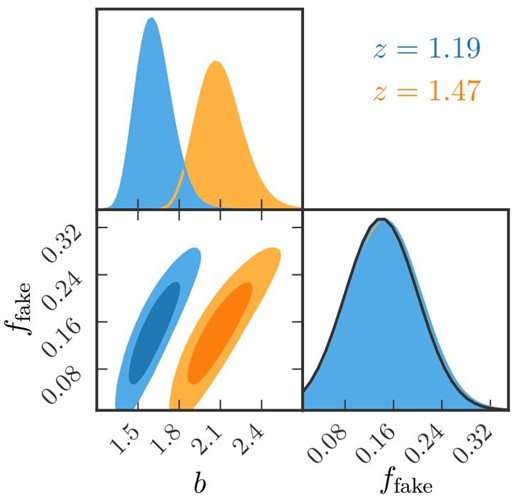
Figure 3 shows the joint constraints on the power-law parameters and the fake line fraction, (A_w, β, f_fake), with blue and orange contours for z = 1.19 and z = 1.47, respectively.⁶ The parameter set with the minimum value of χ² for z = 1.19 is (A_w, β, f_fake) = (1.10, 0.534, 0.140), while that for z = 1.47 is (A_w, β, f_fake) = (1.17, 0.538, 0.139). With these sets of the best-fitting parameters we derive the integral constraints as |$w_\Omega = 0.110$| and |$w_\Omega = 0.114$|⁠, for lower and higher redshifts, respectively. The best-fitting power-law model prediction for the measured correlation function, |$(1-f_{\rm fake})^2(A_w\theta ^{-\beta }-w_\Omega )$|⁠, is shown by the blue line in figure 2. The constrained parameters are shown in table 2.

$Constraints on the power-law model parameters (Aw, β) and the fake line fraction parameter ffake from the angular clustering of [O ii] emitters for z = 1.19 (blue) and z = 1.47 (orange). The contours show the $68\%$ and $95\%$ confidence levels. The diagonal panel shows the posterior probability distribution of each parameter. A Gaussian prior is adopted for the fake line fraction, ffake = 0.140 ± 0.060, which is shown as the black curve compared with the one-dimensional posterior. The posterior of ffake for z = 1.47 (orange) is almost entirely behind that for z = 1.19. (Color online)$

Fig. 3.

Constraints on the power-law model parameters (A_w, β) and the fake line fraction parameter f_fake from the angular clustering of [O ii] emitters for z = 1.19 (blue) and z = 1.47 (orange). The contours show the |$68\%$| and |$95\%$| confidence levels. The diagonal panel shows the posterior probability distribution of each parameter. A Gaussian prior is adopted for the fake line fraction, f_fake = 0.140 ± 0.060, which is shown as the black curve compared with the one-dimensional posterior. The posterior of f_fake for z = 1.47 (orange) is almost entirely behind that for z = 1.19. (Color online)

Table 2.

Parameter constraints on single power-law and linearly biased dark matter models.*

		NB816		NB921
	Prior	Best fit	Posterior PDF	Best fit	Posterior PDF
Power-law parameter
A_w (at 1′)	None	1.10	\|$1.12^{ + 0.21} _{- 0.16}$\|	1.17	\|$1.20^{ + 0.20}_{ - 0.17}$\|
β	None	0.534	\|$0.533 ^{+ 0.057}_{ - 0.055}$\|	0.538	\|$0.537^{+ 0.044}_{ - 0.043}$\|
f_fake	0.140 ± 0.060	0.140	\|$0.149^{ + 0.059}_{ - 0.059}$\|	0.139	\|$0.149^{ + 0.060}_{ - 0.059}$\|
r₀(h⁻¹ Mpc)	—	4.08	\|$4.12^{ + 0.50}_{ - 0.41}$\|	4.55	\|$4.61^{+ 0.51}_{- 0.45}$\|
Linearly biased DM parameter
b	None	1.60	\|$1.61 ^{+ 0.13}_{ - 0.11}$\|	2.08	\|$2.09^{ + 0.17}_{ - 0.15}$\|
f_fake	0.140 ± 0.060	0.140	\|$0.145^{ + 0.059}_{ - 0.059}$\|	0.140	\|$0.145^{ + 0.060}_{ - 0.059}$\|

		NB816		NB921
	Prior	Best fit	Posterior PDF	Best fit	Posterior PDF
Power-law parameter
A_w (at 1′)	None	1.10	\|$1.12^{ + 0.21} _{- 0.16}$\|	1.17	\|$1.20^{ + 0.20}_{ - 0.17}$\|
β	None	0.534	\|$0.533 ^{+ 0.057}_{ - 0.055}$\|	0.538	\|$0.537^{+ 0.044}_{ - 0.043}$\|
f_fake	0.140 ± 0.060	0.140	\|$0.149^{ + 0.059}_{ - 0.059}$\|	0.139	\|$0.149^{ + 0.060}_{ - 0.059}$\|
r₀(h⁻¹ Mpc)	—	4.08	\|$4.12^{ + 0.50}_{ - 0.41}$\|	4.55	\|$4.61^{+ 0.51}_{- 0.45}$\|
Linearly biased DM parameter
b	None	1.60	\|$1.61 ^{+ 0.13}_{ - 0.11}$\|	2.08	\|$2.09^{ + 0.17}_{ - 0.15}$\|
f_fake	0.140 ± 0.060	0.140	\|$0.145^{ + 0.059}_{ - 0.059}$\|	0.140	\|$0.145^{ + 0.060}_{ - 0.059}$\|

*

The values in the “Prior” column quote the mean and standard deviation of the Gaussian priors. The “Best fit” column shows the parameter set which gives the minimum value of χ². In the “Posterior PDF” column the central value is a median and the error means the 16th–84th percentiles after the other parameters are marginalized over.

Table 2.

Parameter constraints on single power-law and linearly biased dark matter models.*

		NB816		NB921
	Prior	Best fit	Posterior PDF	Best fit	Posterior PDF
Power-law parameter
A_w (at 1′)	None	1.10	\|$1.12^{ + 0.21} _{- 0.16}$\|	1.17	\|$1.20^{ + 0.20}_{ - 0.17}$\|
β	None	0.534	\|$0.533 ^{+ 0.057}_{ - 0.055}$\|	0.538	\|$0.537^{+ 0.044}_{ - 0.043}$\|
f_fake	0.140 ± 0.060	0.140	\|$0.149^{ + 0.059}_{ - 0.059}$\|	0.139	\|$0.149^{ + 0.060}_{ - 0.059}$\|
r₀(h⁻¹ Mpc)	—	4.08	\|$4.12^{ + 0.50}_{ - 0.41}$\|	4.55	\|$4.61^{+ 0.51}_{- 0.45}$\|
Linearly biased DM parameter
b	None	1.60	\|$1.61 ^{+ 0.13}_{ - 0.11}$\|	2.08	\|$2.09^{ + 0.17}_{ - 0.15}$\|
f_fake	0.140 ± 0.060	0.140	\|$0.145^{ + 0.059}_{ - 0.059}$\|	0.140	\|$0.145^{ + 0.060}_{ - 0.059}$\|

		NB816		NB921
	Prior	Best fit	Posterior PDF	Best fit	Posterior PDF
Power-law parameter
A_w (at 1′)	None	1.10	\|$1.12^{ + 0.21} _{- 0.16}$\|	1.17	\|$1.20^{ + 0.20}_{ - 0.17}$\|
β	None	0.534	\|$0.533 ^{+ 0.057}_{ - 0.055}$\|	0.538	\|$0.537^{+ 0.044}_{ - 0.043}$\|
f_fake	0.140 ± 0.060	0.140	\|$0.149^{ + 0.059}_{ - 0.059}$\|	0.139	\|$0.149^{ + 0.060}_{ - 0.059}$\|
r₀(h⁻¹ Mpc)	—	4.08	\|$4.12^{ + 0.50}_{ - 0.41}$\|	4.55	\|$4.61^{+ 0.51}_{- 0.45}$\|
Linearly biased DM parameter
b	None	1.60	\|$1.61 ^{+ 0.13}_{ - 0.11}$\|	2.08	\|$2.09^{ + 0.17}_{ - 0.15}$\|
f_fake	0.140 ± 0.060	0.140	\|$0.145^{ + 0.059}_{ - 0.059}$\|	0.140	\|$0.145^{ + 0.060}_{ - 0.059}$\|

*

The values in the “Prior” column quote the mean and standard deviation of the Gaussian priors. The “Best fit” column shows the parameter set which gives the minimum value of χ². In the “Posterior PDF” column the central value is a median and the error means the 16th–84th percentiles after the other parameters are marginalized over.

When the two parameters for a power-law model of the angular correlation, (A_w, β), are known, one can determine its three-dimensional clustering, ξ(r) = (r/r₀)^−γ, as (Peebles 1980; Efstathiou et al. 1991; Simon 2007)

$$\begin{eqnarray} A_w &=& r_0^\gamma \left( \frac{10800}{\pi } \right)^{\gamma -1} B\left( \frac{1}{2},\frac{\gamma -1}{2} \right)\int ^\infty _0 dx p^2(x) x^{1-\gamma } \nonumber \\ &=&r_0^\gamma \frac{10800^{\gamma -1}\left(x_{\rm max}^{\gamma -1}-x_{\rm min}^{\gamma -1}\right)}{\pi ^{\gamma -1}(2-\gamma )(x_{\rm max}-x_{\rm min})^2} B\left( \frac{1}{2},\frac{\gamma -1}{2} \right), \end{eqnarray}$$

(15)

$$\begin{eqnarray} \beta &=& \gamma -1, \end{eqnarray}$$

(16)

where B is the beta function. The final expression for A_w is derived using the constant radial selection function [equation (10)]. As a result, the clustering length is constrained to be |$r_0= 4.12^{+0.50}_{-0.41}$| at z = 1.19 and |$r_0= 4.61^{+0.51}_{-0.45}$| at z = 1.47. These values correspond to host halo masses of M ≳ 10¹² h⁻¹ M_⊙ and are roughly consistent with the preceding results for ELG clustering (see, e.g., Kashino et al. 2017). Here we do not make a detailed comparison with previous works nor discuss the clustering evolution further because the power-law model is not accurate enough to be used to interpret the precise correlation function measurement. In section 5 we discuss the physical properties of halos hosting ELGs based on an HOD model that is much more sophisticated than the power-law model.

4.3 Linearly biased dark matter model

Next, we consider another simple model, the non-linear correlation function with the linear galaxy bias factor (Kaiser 1984),

$$\begin{equation} \xi (r;b)=b^2\xi _{\rm m}(r), \end{equation}$$

(17)

where ξ_m is the underlying matter correlation function. We use the fitting formula of Takahashi et al. (2012) to compute the non-linear matter power spectrum, P_m(k), and then Fourier transform it to obtain ξ_m. Given equation (17), a similar form is derived for the angular correlation function as

$$\begin{equation} w(\theta ;b)=b^2w_{\rm m}(\theta ), \end{equation}$$

(18)

where w_m is the angular correlation function of matter, calculated using equation (9) with ξ(r) replaced by the three-dimensional matter correlation function, ξ_m(r). In this model there are two free parameters to be determined, Θ = (b, f_fake). This model is valid for a wider range of angular scales than the single power-law model. The data at the scales |$0{_{.}^{\circ}} 0025 < \theta < 1 $|° are used to calculate the χ² statistic (N_bin = 13).

The joint constraints on (b, f_fake) are shown in figure 4. We find the best-fitting value of the bias parameter, |$b= 1.61 ^{+ 0.13}_{ - 0.11}$| and |$b= 2.09^{ + 0.17}_{ - 0.15}$|⁠, respectively for the lower- and higher-redshift measurements. These bias values can be compared to the effective bias b_eff to be determined by HOD modeling [equation (27)]. The integral constraint is calculated by these best-fitting parameter sets for the correlation in the combined field as |$w_\Omega = 0.0270$| and |$w_\Omega = 0.0277$| for z = 1.19 and 1.47, respectively.

$Constraints on the linear galaxy bias b of the non-linear dark matter model and the fake line fraction parameter ffake for z = 1.19 (blue) and z = 1.47 (orange). The contours show the $68\%$ and $95\%$ confidence levels. The diagonal panels show the posterior probability distribution of each parameter. A Gaussian prior is adopted for the fake line fraction, ffake = 0.140 ± 0.060, which is shown as the black curve compared with the one-dimensional posterior. The posterior of ffake for z = 1.47 (orange) is almost entirely behind that for z = 1.19. (Color online)$

Fig. 4.

Constraints on the linear galaxy bias b of the non-linear dark matter model and the fake line fraction parameter f_fake for z = 1.19 (blue) and z = 1.47 (orange). The contours show the |$68\%$| and |$95\%$| confidence levels. The diagonal panels show the posterior probability distribution of each parameter. A Gaussian prior is adopted for the fake line fraction, f_fake = 0.140 ± 0.060, which is shown as the black curve compared with the one-dimensional posterior. The posterior of f_fake for z = 1.47 (orange) is almost entirely behind that for z = 1.19. (Color online)

The best-fitting linearly biased dark matter model, |$(1-f_{\rm fake})^2[b^2w_{\rm m}(\theta )-w_\Omega ]$|⁠, is shown as the red solid curve in figure 2. To see the contribution of the integral constraint, we show the same model without the |$w_\Omega$| term, (1 − f_fake)²b²w_m(θ), as the red dashed curve. As expected, the model correlation function is positive over all the scales studied here. As a reference, the dark matter correlation function, w_m, is shown by the black dashed curve in figure 2.

The relatively large uncertainties on the bias parameter come from our conservative prior on f_fake. To see this, let us directly constrain the observed amplitude by considering the relation

$$\begin{eqnarray} \hat{w}(\theta ;\tilde{b}) &=& \tilde{w}(\theta ;\tilde{b})-\tilde{w}_\Omega (\tilde{b}) \nonumber \\ &=& \tilde{w}(\theta ;\tilde{b}) - \frac{\sum _i{\tilde{w}(\theta _i;\tilde{b})RR(\theta _i)}}{\sum _i{RR(\theta _i)}}, \end{eqnarray}$$

(19)

where |$\tilde{b}$| is the bias parameter of the observed field, |$\tilde{w}(\theta ,\tilde{b}) = \tilde{b}^2w_{\rm m}(\theta )$|⁠. Equation (19) becomes equivalent to equations (6) and (18) if we set |$\tilde{b} \equiv (1-f_{\rm fake})b$|⁠. By adopting this one-parameter linearly biased dark matter model, we obtain tighter constraints as |$\tilde{b} = 1.379^{+0.042}_{-0.043}$| and |$\tilde{b} = 1.786 ^{+0.052}_{-0.054}$| at z = 1.19 and z = 1.47, respectively, without any prior.

In the next subsection we further analyze the [O ii] emitter samples with different luminosity and stellar mass thresholds using the linearly biased DM model.

4.4 Line luminosity and stellar mass dependencies of [O ii]-emitter clustering

It is interesting to see how the amplitude of a measured correlation function depends on the properties of the [O ii] emitters. Here we consider two basic properties, the luminosity of the [O ii] emission line and the stellar mass of the host galaxies, and split our sample into subsamples based on these thresholds.

Figure 5 shows the angular correlation functions measured with different line luminosity cuts. For clarity, we add the integral constraint correction so that all the correlation functions become positive at all scales probed. For each correlation function, we perform a model fitting using the linearly biased dark matter model considered in subsection 4.3. The best-fitting model for each measurement, (1 − f_fake)²b²w_m(θ), is presented by the dashed curve. As discussed in subsection 4.3, this simple model fails to explain the measured correlation function at small scales. To see the dependence of the clustering amplitude on the luminosity, we constrain the parameter |$\tilde{b}$| in equation (19) as a function of the minimum line luminosity L_min. The result is shown in the left panel of figure 6. For each redshift, we find that the bias b increases with increasing line luminosity, by ∼10%. If the fake line fraction, f_fake, changed significantly with the luminosity, this luminosity dependence would be modulated.

$Angular correlation functions of [O ii] emitters at z = 1.19 (top) and z = 1.47 (bottom) with different peak luminosity cuts. The unit of L in the legend is [erg s−1]. For visualization purposes, the integral constraint is taken into account, and thus the vertical axis represents $\hat{w}+(1-f_{\rm fake})^2w_\Omega$. The amplitudes of the correlation functions shown by the blue, green, yellow, brown, and purple points are multiplied by 2n, where n = 1, 2, …, 5, respectively. The dashed curves are the best-fitting models of the linearly biased dark matter model, (1 − ffake)2b2wm(θ). (Color online)$

Fig. 5.

Angular correlation functions of [O ii] emitters at z = 1.19 (top) and z = 1.47 (bottom) with different peak luminosity cuts. The unit of L in the legend is [erg s⁻¹]. For visualization purposes, the integral constraint is taken into account, and thus the vertical axis represents |$\hat{w}+(1-f_{\rm fake})^2w_\Omega$|⁠. The amplitudes of the correlation functions shown by the blue, green, yellow, brown, and purple points are multiplied by 2ⁿ, where n = 1, 2, …, 5, respectively. The dashed curves are the best-fitting models of the linearly biased dark matter model, (1 − f_fake)²b²w_m(θ). (Color online)

$Constraints on the measured clustering amplitude of [O ii] emitters, $\tilde{b}=(1-f_{\rm fake})b$, as a function of the minimum peak luminosity Lmin (left) and stellar mass M*, min (right). The blue and orange points are the results at z = 1.19 and z = 1.47, respectively. (Color online)$

Fig. 6.

Constraints on the measured clustering amplitude of [O ii] emitters, |$\tilde{b}=(1-f_{\rm fake})b$|⁠, as a function of the minimum peak luminosity L_min (left) and stellar mass M_{*, min} (right). The blue and orange points are the results at z = 1.19 and z = 1.47, respectively. (Color online)

We repeat the same analysis by splitting our [O ii] emitter sample into subsamples with stellar mass cuts M_{*, min}. We measure the angular correlation function of [O ii] emitters with stellar mass M_* ≥ M_{*, min}. Since the fitting result for w(θ) is similar to that with the luminosity cuts in figure 5, we do not plot the figure. We constrain the measured clustering amplitude |$\tilde{b}$| as a function of M_{*, min}, as shown in the right panel of figure 6. A trend similar to the line luminosity limited samples is found: [O ii] emitters with higher stellar masses cluster more strongly than those with lower masses. Almost no mass dependence is seen in the clustering at z = 1.47. As discussed in subsection 3.6 of Hayashi et al. (2018), multi-band data at longer wavelengths, such as near-infrared data, would be required to accurately estimate the stellar masses at z ∼ 1.5. Thus, our result for the stellar mass dependence of the clustering at z = 1.47 needs to be interpreted with caution. Overall, however, the dependence of the clustering of [O ii] emitters on stellar masses is not as strong as on line luminosities, which is qualitatively consistent with the result of Khostovan et al. (2018).

5 Dark matter–[O ii] emitter connections

Halo occupation distribution modeling is an empirical and parametric way to describe the connection between galaxies and their host halos through modeling the abundance and clustering of galaxies (Jing et al. 1998; Peacock & Smith 2000; Seljak 2000; Ma & Fry 2000; Scoccimarro et al. 2001; Cooray & Sheth 2002; Berlind & Weinberg 2002; Zheng et al. 2005; van den Bosch et al. 2013; Hikage et al. 2013; Okumura et al. 2015). In this section we use HOD modeling to investigate physical properties of halos which host [O ii] emitters.

5.1 Formalism of halo model

The mean number of galaxies residing in a halo of mass M, denoted as 〈N(M)〉, is decomposed into central and satellite components,

$$\begin{eqnarray} && \left\langle N(M) \right\rangle = \left\langle N_{\rm cen}(M)\right\rangle + \left\langle N_{\rm sat}(M)\right\rangle . \end{eqnarray}$$

(20)

Once the HOD model is specified, the average number density of galaxies is calculated as

$$\begin{equation} n_{\rm g}=\int \left\langle N(M) \right\rangle n(M)dM, \end{equation}$$

(21)

where n(M)dM is the halo mass function.

In a halo model approach, the power spectrum of galaxies, P(k), where k is the wavenumber, can be decomposed into one- and two-halo terms,

$$\begin{equation} P(k)=P_{1h}(k)+P_{2h}(k). \end{equation}$$

(22)

The one-halo term can be further decomposed into contributions from the clustering of central–satellite and satellite–satellite pairs hosted by the same halos, namely

$$\begin{eqnarray} P_{1h}(k) &=& \frac{1}{n_{\rm g}^2}\int n(M)dM \left[ 2\left\langle N_{\rm cen}N_{\rm sat} \right\rangle u(k,M) \right. \nonumber \\ && \left. + \left\langle N_{\rm sat}(N_{\rm sat}-1) \right\rangle u ^2 (k,M)\right], \end{eqnarray}$$

(23)

where u(k, M) describes the Fourier transform of the density profile of satellite galaxies within dark matter halos, which is assumed to follow the matter density profile. We assume that N_sat follows Poisson statistics such that 〈N_sat(N_sat − 1)〉 = 〈N_sat〉². We also assume that the occupation numbers of central and satellite galaxies are independent, i.e., 〈N_cenN_sat〉 = 〈N_cen〉〈N_sat〉. The two-halo term can be similarly decomposed into central–central, central–satellite, and satellite–satellite galaxy pairs hosted by distinct halos,

$$\begin{eqnarray} P_{2h}(k) &=& \frac{1}{n_{\rm g}^2}\int n(M)dM \int n(M^{\prime })dM^{\prime } \nonumber \\ && \times \left[ \left\langle N_{\rm cen} \right\rangle + \left\langle N_{\rm sat}\right\rangle u(k,M)\right] \nonumber \\ && \times \left[ \left\langle N_{\rm cen} \right\rangle + \left\langle N_{\rm sat}\right\rangle u(k,M^{\prime })\right] P_{hh}(k;M,M^{\prime }), \end{eqnarray}$$

(24)

where P_hh(k; M, M′) is the cross-power spectrum of halos with masses M and M′. The halo mass function is calculated using the model derived by Tinker et al. (2010). The density profile of halos is assumed to be NFW (Navarro et al. 1997) with the concentration given by Duffy et al. (2008). We compute P_hh as a product of the non-linear matter power spectrum (Takahashi et al. 2012) and the halo bias,

$$\begin{equation} P_{hh}(k;M,M^{\prime }) = b_{\rm h}(M)b_{\rm h}(M^{\prime })P_m(k), \end{equation}$$

(25)

where b_h(M) is the bias for a halo of mass M. We use the large-scale halo bias b_h(M) also proposed by Tinker et al. (2010).

The three-dimensional correlation function for galaxies is calculated by a Fourier transform of the power spectrum,

$$\begin{equation} \xi (r) = \frac{1}{2\pi ^2} \int ^\infty _0 dkk^2P(k) \frac{\sin {kr}}{kr}. \end{equation}$$

(26)

Then, the angular correlation function is finally obtained through equation (9).

In addition to the number density, given a set of HOD parameters, one can determine various physical quantities such as the effective bias,

$$\begin{equation} b_{\rm eff} = \frac{1}{n_{\rm g}}\int b_{\rm h}(M) \left\langle N(M) \right\rangle n(M)dM, \end{equation}$$

(27)

the effective halo mass,

$$\begin{equation} M_{\rm eff} = \frac{1}{n_{\rm g}}\int M\left\langle N(M) \right\rangle n(M) dM, \end{equation}$$

(28)

and the satellite fraction,

$$\begin{equation} f_{\rm sat} = \frac{1}{n_{\rm g}} \int \left\langle N_{\rm sat}(M) \right\rangle n(M) dM. \end{equation}$$

(29)

5.2 Halo occupation distribution model for [O ii] emitters

In this paper we adopt the HOD model developed by Geach et al. (2012) to describe the population of ELGs (see also Kim et al. 2011; Contreras et al. 2013). In this model, the central HOD is described by two components:

$$\begin{eqnarray} \left\langle N_{\rm cen}(M)\right\rangle &=& F_c^B(1-F_c^A) \exp {\left[ -\frac{\log {(M/M_{\rm c})}^2}{2(\sigma _{\log {M}})^2} \right]} \nonumber \\ && +\, F_c^A \left\lbrace 1+{\rm erf} \left[\frac{\log {(M/M_{\rm c})}}{\sigma _{\log {M}}}\right] \right\rbrace , \end{eqnarray}$$

(30)

where |$F_c^{A,B}$| are normalization factors. The first component describes the Gaussian distribution of centrals around halos of average mass M_c with dispersion σ_log M, and the second component describes the standard mass-limited step function form proposed by Zheng et al. (2005), see subsection 5.5 below. The satellite HOD is given by

$$\begin{equation} \left\langle N_{\rm sat}(M) \right\rangle \!=\! F_{\rm s} \left\lbrace 1+{\rm erf} \left[\frac{\log {(M/M_{\rm min})}}{\delta _{\log {M}}}\right] \right\rbrace \left( \frac{M}{M_{\rm min}}\right)^\alpha , \end{equation}$$

(31)

where F_s is the mean number of satellites per halo at the transition mass M_min that corresponds to the characteristic mass above which halos can contain satellites, δ_log M is the width of the transition from zero satellites per halo to the power law, and α is the slope of the power law, which gives the mean number of satellites for M > M_min. We refer the reader to Geach et al. (2012) and Contreras et al. (2013) for a more detailed explanation of this model.

We fix the least important parameter, δ_log M, to δ_log M = 1. Thus, the number of free parameters in the Geach HOD model together with the fake line fraction is eight: |$\Theta = (M_{\rm c}, M_{\rm min}, \sigma _{\log {M}}, \alpha , F_c^A, F_c^B, F_{\rm s}, f_{\rm fake})$|⁠. The parameter α is known to have a value around unity. We thus apply a Gaussian prior on α as α = 1.00 ± 0.20. As with the analysis in section 4, we further impose a Gaussian prior on the fake line fraction parameter as f_fake = 0.140 ± 0.060. Uniform priors are applied for the other six parameters. Table 3 summarizes the priors on all eight parameters. We use the Python package HALOMOD (Murray et al. 2013) to calculate the HOD model prediction for the angular correlation function.

Table 3.

Priors and constraints of the HOD parameters for the Geach model.*

		NB816		NB921
		Best fit	Posterior PDF	Best fit	Posterior PDF
Parameter	Prior
log M_c/(h⁻¹ M_⊙)	None	11.75	\|$12.04^{+0.57}_{-0.32}$\|	11.93	\|$11.91^{+ 0.19} _{- 0.18}$\|
log M_min/(h⁻¹ M_⊙)	None	12.46	\|$12.61^{+0.32}_{-0.43}$\|	12.47	\|$12.57^{+0.29}_{-0.35}$\|
σ_log M	[0,1]	0.06	\|$0.40^{+0.28}_{-0.31}$\|	0.13	\|$0.17^{+ 0.15}_{- 0.10}$\|
α	1.00 ± 0.20	1.06	\|$1.03^{+0.12}_{-0.13}$\|	1.23	\|$1.12^{+ 0.13}_{- 0.12}$\|
\|$F_c^A$\|	[0, 0.5]	0.13	\|$0.26^{+0.16}_{-0.12}$\|	0.14	\|$0.26^{+ 0.15}_{- 0.13}$\|
\|$F_c^B$\|	[0,1]	0.95	\|$0.37^{+0.39}_{-0.28}$\|	0.90	\|$0.53^{+ 0.32}_{- 0.34}$\|
F_s	[0, 1]	0.98	\|$0.54^{+0.31}_{-0.34}$\|	0.73	\|$0.55^{+ 0.31}_{- 0.33}$\|
f_fake	0.140 ± 0.060	0.172	\|$0.140^{+0.048}_{-0.053}$\|	0.128	\|$0.104^{+ 0.043}_{- 0.041}$\|
χ²/ν (ν = 7)		2.17		0.856
Inferred quantity	Measurement
log n_g/(h⁻¹ Mpc)⁻³	−2.259 ± 0.068 (NB816)	−2.313	\|$-2.316^{+0.071}_{-0.073}$\|	−2.401	\|$-2.381^{+0.074}_{-0.073}$\|
	−2.344 ± 0.070 (NB921)
f_sat	—	0.308	\|$0.159^{+0.120}_{-0.047}$\|	0.242	\|$0.159^{ + 0.109}_{ - 0.049}$\|
b_eff	—	1.797	\|$1.700^{+0.084}_{-0.111}$\|	2.029	\|$1.981^{+0.072}_{-0.068}$\|
log M_eff/(h⁻¹ M_⊙)	—	12.831	\|$12.703^{+0.093}_{-0.071}$\|	12.699	\|$12.609^{+0.085}_{-0.051}$\|

		NB816		NB921
		Best fit	Posterior PDF	Best fit	Posterior PDF
Parameter	Prior
log M_c/(h⁻¹ M_⊙)	None	11.75	\|$12.04^{+0.57}_{-0.32}$\|	11.93	\|$11.91^{+ 0.19} _{- 0.18}$\|
log M_min/(h⁻¹ M_⊙)	None	12.46	\|$12.61^{+0.32}_{-0.43}$\|	12.47	\|$12.57^{+0.29}_{-0.35}$\|
σ_log M	[0,1]	0.06	\|$0.40^{+0.28}_{-0.31}$\|	0.13	\|$0.17^{+ 0.15}_{- 0.10}$\|
α	1.00 ± 0.20	1.06	\|$1.03^{+0.12}_{-0.13}$\|	1.23	\|$1.12^{+ 0.13}_{- 0.12}$\|
\|$F_c^A$\|	[0, 0.5]	0.13	\|$0.26^{+0.16}_{-0.12}$\|	0.14	\|$0.26^{+ 0.15}_{- 0.13}$\|
\|$F_c^B$\|	[0,1]	0.95	\|$0.37^{+0.39}_{-0.28}$\|	0.90	\|$0.53^{+ 0.32}_{- 0.34}$\|
F_s	[0, 1]	0.98	\|$0.54^{+0.31}_{-0.34}$\|	0.73	\|$0.55^{+ 0.31}_{- 0.33}$\|
f_fake	0.140 ± 0.060	0.172	\|$0.140^{+0.048}_{-0.053}$\|	0.128	\|$0.104^{+ 0.043}_{- 0.041}$\|
χ²/ν (ν = 7)		2.17		0.856
Inferred quantity	Measurement
log n_g/(h⁻¹ Mpc)⁻³	−2.259 ± 0.068 (NB816)	−2.313	\|$-2.316^{+0.071}_{-0.073}$\|	−2.401	\|$-2.381^{+0.074}_{-0.073}$\|
	−2.344 ± 0.070 (NB921)
f_sat	—	0.308	\|$0.159^{+0.120}_{-0.047}$\|	0.242	\|$0.159^{ + 0.109}_{ - 0.049}$\|
b_eff	—	1.797	\|$1.700^{+0.084}_{-0.111}$\|	2.029	\|$1.981^{+0.072}_{-0.068}$\|
log M_eff/(h⁻¹ M_⊙)	—	12.831	\|$12.703^{+0.093}_{-0.071}$\|	12.699	\|$12.609^{+0.085}_{-0.051}$\|

*

In the “Prior” column the ranges specified in brackets are for uniform priors while for the others we quote the mean and standard deviation of the Gaussian priors. The “Best fit” column shows the parameter set which gives the minimum value of χ². In the “Posterior PDF” column the central value is a median and the error means the 16th–84th percentiles after the other parameters are marginalized over. The measured number density log n_g includes non-[O ii] emitters, and thus its best-fitting values differ from the measure ones by log (1 − f_fake) ∼ −0.06.

Table 3.

Priors and constraints of the HOD parameters for the Geach model.*

		NB816		NB921
		Best fit	Posterior PDF	Best fit	Posterior PDF
Parameter	Prior
log M_c/(h⁻¹ M_⊙)	None	11.75	\|$12.04^{+0.57}_{-0.32}$\|	11.93	\|$11.91^{+ 0.19} _{- 0.18}$\|
log M_min/(h⁻¹ M_⊙)	None	12.46	\|$12.61^{+0.32}_{-0.43}$\|	12.47	\|$12.57^{+0.29}_{-0.35}$\|
σ_log M	[0,1]	0.06	\|$0.40^{+0.28}_{-0.31}$\|	0.13	\|$0.17^{+ 0.15}_{- 0.10}$\|
α	1.00 ± 0.20	1.06	\|$1.03^{+0.12}_{-0.13}$\|	1.23	\|$1.12^{+ 0.13}_{- 0.12}$\|
\|$F_c^A$\|	[0, 0.5]	0.13	\|$0.26^{+0.16}_{-0.12}$\|	0.14	\|$0.26^{+ 0.15}_{- 0.13}$\|
\|$F_c^B$\|	[0,1]	0.95	\|$0.37^{+0.39}_{-0.28}$\|	0.90	\|$0.53^{+ 0.32}_{- 0.34}$\|
F_s	[0, 1]	0.98	\|$0.54^{+0.31}_{-0.34}$\|	0.73	\|$0.55^{+ 0.31}_{- 0.33}$\|
f_fake	0.140 ± 0.060	0.172	\|$0.140^{+0.048}_{-0.053}$\|	0.128	\|$0.104^{+ 0.043}_{- 0.041}$\|
χ²/ν (ν = 7)		2.17		0.856
Inferred quantity	Measurement
log n_g/(h⁻¹ Mpc)⁻³	−2.259 ± 0.068 (NB816)	−2.313	\|$-2.316^{+0.071}_{-0.073}$\|	−2.401	\|$-2.381^{+0.074}_{-0.073}$\|
	−2.344 ± 0.070 (NB921)
f_sat	—	0.308	\|$0.159^{+0.120}_{-0.047}$\|	0.242	\|$0.159^{ + 0.109}_{ - 0.049}$\|
b_eff	—	1.797	\|$1.700^{+0.084}_{-0.111}$\|	2.029	\|$1.981^{+0.072}_{-0.068}$\|
log M_eff/(h⁻¹ M_⊙)	—	12.831	\|$12.703^{+0.093}_{-0.071}$\|	12.699	\|$12.609^{+0.085}_{-0.051}$\|

		NB816		NB921
		Best fit	Posterior PDF	Best fit	Posterior PDF
Parameter	Prior
log M_c/(h⁻¹ M_⊙)	None	11.75	\|$12.04^{+0.57}_{-0.32}$\|	11.93	\|$11.91^{+ 0.19} _{- 0.18}$\|
log M_min/(h⁻¹ M_⊙)	None	12.46	\|$12.61^{+0.32}_{-0.43}$\|	12.47	\|$12.57^{+0.29}_{-0.35}$\|
σ_log M	[0,1]	0.06	\|$0.40^{+0.28}_{-0.31}$\|	0.13	\|$0.17^{+ 0.15}_{- 0.10}$\|
α	1.00 ± 0.20	1.06	\|$1.03^{+0.12}_{-0.13}$\|	1.23	\|$1.12^{+ 0.13}_{- 0.12}$\|
\|$F_c^A$\|	[0, 0.5]	0.13	\|$0.26^{+0.16}_{-0.12}$\|	0.14	\|$0.26^{+ 0.15}_{- 0.13}$\|
\|$F_c^B$\|	[0,1]	0.95	\|$0.37^{+0.39}_{-0.28}$\|	0.90	\|$0.53^{+ 0.32}_{- 0.34}$\|
F_s	[0, 1]	0.98	\|$0.54^{+0.31}_{-0.34}$\|	0.73	\|$0.55^{+ 0.31}_{- 0.33}$\|
f_fake	0.140 ± 0.060	0.172	\|$0.140^{+0.048}_{-0.053}$\|	0.128	\|$0.104^{+ 0.043}_{- 0.041}$\|
χ²/ν (ν = 7)		2.17		0.856
Inferred quantity	Measurement
log n_g/(h⁻¹ Mpc)⁻³	−2.259 ± 0.068 (NB816)	−2.313	\|$-2.316^{+0.071}_{-0.073}$\|	−2.401	\|$-2.381^{+0.074}_{-0.073}$\|
	−2.344 ± 0.070 (NB921)
f_sat	—	0.308	\|$0.159^{+0.120}_{-0.047}$\|	0.242	\|$0.159^{ + 0.109}_{ - 0.049}$\|
b_eff	—	1.797	\|$1.700^{+0.084}_{-0.111}$\|	2.029	\|$1.981^{+0.072}_{-0.068}$\|
log M_eff/(h⁻¹ M_⊙)	—	12.831	\|$12.703^{+0.093}_{-0.071}$\|	12.699	\|$12.609^{+0.085}_{-0.051}$\|

*

In the “Prior” column the ranges specified in brackets are for uniform priors while for the others we quote the mean and standard deviation of the Gaussian priors. The “Best fit” column shows the parameter set which gives the minimum value of χ². In the “Posterior PDF” column the central value is a median and the error means the 16th–84th percentiles after the other parameters are marginalized over. The measured number density log n_g includes non-[O ii] emitters, and thus its best-fitting values differ from the measure ones by log (1 − f_fake) ∼ −0.06.

5.3 HOD parameter constraints

We present constraints on the HOD model using the measured angular correlation function of the [O ii] emitters. We compute the χ² statistic for the HOD model constructed from the observed angular correlation function, |$\chi _w^2$|⁠, and number density, |$\chi _n^2$|⁠, as

$$\begin{equation} \chi ^2 (\Theta ) = \chi _w^2 (\Theta ) + \chi _n^2 (\Theta ), \end{equation}$$

(32)

where |$\chi _w^2$| is given by equation (13) and |$\chi _n^2$| is given by

$$\begin{equation} \chi _n^2 (\Theta ) = \frac{\left[\log {n_{\rm g}^{\rm obs}}-\log {n_{\rm g}^{\rm th}(\Theta )}+\log {(1-f_{\rm fake})}\right]^2}{\sigma ^2_{\log {n_{\rm g}}}}, \end{equation}$$

(33)

where |$\Theta = (\log {M_{\rm c}}, \log {M_{\rm min}}, \alpha , \sigma _{\log {M}}, F_{\rm s}, F_c^A,F_c^B,f_{\rm fake})$|⁠. Since the observed number of [O ii] emitters includes non-[O ii] contaminants characterized by the fraction f_fake, we need to take into account a factor of (1 − f_fake) difference between the observed number density and its theoretical prediction computed by equation (21). As shown in table 1, the observed number density is |$n_{\rm g}^{\rm obs} = 5.50 \times 10^{-3} \, (h^{-1}\,{\rm Mpc})^{-3}$| at z = 1.19 and |$n_{\rm g}^{\rm obs} = 4.08 \times 10^{-3} \, (h^{-1}\,{\rm Mpc})^{-3}$| at z = 1.47. We set the uncertainty of |$\log {n_{\rm g}^{\rm obs}}$| as |$\sigma _{\log {n_{\rm g}}} = 0.03 |\log {n_{\rm g}^{\rm obs}}|$| following the measurement uncertainty of the luminosity function (Hayashi et al. 2020). Due to the flexibility of the model, the HOD enables us to fit an observed correlation function over a broader range than the power-law and nonlinear dark matter models considered in the previous section. We thus use the data at |$0{_{.}^{\circ}} 0015 < \theta < 1$|° and the number of angular separation bins is N_bin = 14. Together with the number density, the degree of freedom is ν = N_bin + 1 − 8 = 7.

The resulting constraints on the HOD parameters of the Geach model are shown in figure 7. This and the following two figures are the main results of this paper. The eight-dimensional posterior distributions are visualized in two-dimensional contours with the other six parameters marginalized over. The top row of each column shows the one-dimensional posterior. The constraints are summarized in table 3. The normalization parameters, |$F_c^{A,B}$| and F_s, are poorly constrained, which is expected and consistent with Geach et al. (2012) and Hong et al. (2019). Overall, constraints from the z = 1.47 sample are tighter than those from the z = 1.19 one. In particular, the marginalized distribution for σ_log M for the z = 1.19 sample is much wider and even becomes bimodal. Interestingly, this bimodality was seen by Hong et al. (2019) who analyzed the clustering of Lyα emitters using the Geach HOD model. Although there are many free parameters with few priors, we obtain meaningful constraints due to our large sample. Particularly strong constrains are obtained for the two mass parameters, M_c and M_min, as seen in table 3, because M_c can be determined by the observed number density, n_g, and M_min primarily degenerates with M_c. We do not see a strong evolution of HOD from z = 1.47 to 1.19, which is consistent with our ongoing work based on cosmological hydrodynamical simulations (K. Osato & T. Okumura in preparation).

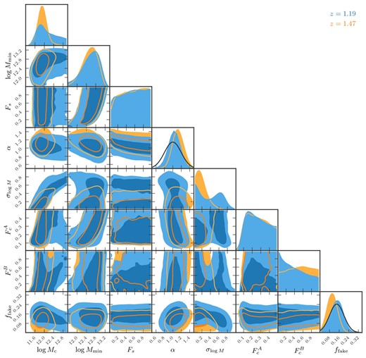
$Constraints on parameters of the Geach HOD model, $(\log {M_{\rm c}}, \log {M_{\rm min}}, \alpha , \sigma _{\log {M}}, F_{\rm s}, F_c^A,F_c^B)$ and ffake, for z = 1.19 (blue) and z = 1.47 (orange). Two-dimensional contours show the $68\%$ and $95\%$ confidence levels after the other six parameters are marginalized over. The diagonal panels show the posterior probability distribution of each parameter. Gaussian priors are assumed for α and ffake, as depicted by the black sold curves in the one-dimensional posterior panels. (Color online)$

Fig. 7.

Constraints on parameters of the Geach HOD model, |$(\log {M_{\rm c}}, \log {M_{\rm min}}, \alpha , \sigma _{\log {M}}, F_{\rm s}, F_c^A,F_c^B)$| and f_fake, for z = 1.19 (blue) and z = 1.47 (orange). Two-dimensional contours show the |$68\%$| and |$95\%$| confidence levels after the other six parameters are marginalized over. The diagonal panels show the posterior probability distribution of each parameter. Gaussian priors are assumed for α and f_fake, as depicted by the black sold curves in the one-dimensional posterior panels. (Color online)

The posterior distribution of the HOD is shown in figure 8. The dark and light shaded regions show the 68% and 95% confidence intervals for the total HOD, respectively, and the red solid curve is the median. The black solid curve is the HOD with a set of parameters which give the minimum χ² value in the eight-dimensional parameter space. The HOD with the minimum χ² looks somewhat different from the median of the HOD, particularly the central HOD. This is a similar trend to that found by Hong et al. (2019). They found that two independent algorithms give very different best-fitting HOD parameters (see Model#1 and Model#2 of their figure 7). This small but non-negligible discrepancy largely comes from the fact that the normalization parameters, especially |$F_c^B$|⁠, and the scatter of the mass, σ_log M, are poorly constrained. Even though the HODs are different, the predicted angular correlation functions with these HOD parameter sets become very similar.

$HOD with the best-fitting parameters of the Geach model at z = 1.19 (top) and z = 1.47 (bottom). The blue and yellow lines show the average numbers of centrals from the Gaussian and error function terms [see equation (30)], while the green line shows that of satellites. The red solid line is the sum of the blue, yellow, and green lines, the average number of all the [O ii] emitters. The dark and light red shaded regions indicate the $68\%$ and $95\%$ confidence intervals. The red dashed curve is the same as the red solid curve but for the best-fitting HOD of Zheng et al. (2005). For comparison, the black curve shows the HOD of the Geach model which gives the minimum χ2 value. (Color online)$

Fig. 8.

HOD with the best-fitting parameters of the Geach model at z = 1.19 (top) and z = 1.47 (bottom). The blue and yellow lines show the average numbers of centrals from the Gaussian and error function terms [see equation (30)], while the green line shows that of satellites. The red solid line is the sum of the blue, yellow, and green lines, the average number of all the [O ii] emitters. The dark and light red shaded regions indicate the |$68\%$| and |$95\%$| confidence intervals. The red dashed curve is the same as the red solid curve but for the best-fitting HOD of Zheng et al. (2005). For comparison, the black curve shows the HOD of the Geach model which gives the minimum χ² value. (Color online)

The best-fitting Geach HOD model prediction, |$(1-f_{\rm fake})^2[w(\theta ;\Theta )-w_\Omega ]$|⁠, is shown as the red solid curve in figure 9. The contributions from the one- and two-halo components are shown as the blue and green curves, respectively. Obviously, agreement of the measured correlation function with the HOD model prediction is much more remarkable than that with the power-law or linearly biased dark matter model, compared to figure 2.

$Angular correlation functions of [O ii] emitters at z = 1.19 (top) and z = 1.47 (bottom). Note that the vertical axis mixes logarithmic and linear scalings. The red points are the measurement, $\hat{w}$, the same as those in figure 2. The blue and green solid curves are the one- and two-halo terms with the best-fitting Geach HOD model, respectively, and the red solid curve is their sum. For comparison, we also show the best-fitting Zheng HOD model as the red dashed curve. The data enclosed by the two red vertical lines are used for this HOD analysis. (Color online)$

Fig. 9.

Angular correlation functions of [O ii] emitters at z = 1.19 (top) and z = 1.47 (bottom). Note that the vertical axis mixes logarithmic and linear scalings. The red points are the measurement, |$\hat{w}$|⁠, the same as those in figure 2. The blue and green solid curves are the one- and two-halo terms with the best-fitting Geach HOD model, respectively, and the red solid curve is their sum. For comparison, we also show the best-fitting Zheng HOD model as the red dashed curve. The data enclosed by the two red vertical lines are used for this HOD analysis. (Color online)

5.4 Derived physical parameters for host halos

Using the constrained HOD parameters, one can infer the parameters which characterize the properties of [O ii] emitters and their host dark matter halos, such as the galaxy number density, effective halo bias and mass, and satellite galaxy fraction, through equations (21), (27), (28), and (29), respectively. The posterior distribution for these parameters is shown in figure 10 and summarized in table 3. The number density is constrained following the imposed prior. Note again that the constrained number density is different from the observed number density by a factor of (1 − f_fake), |$n_{\rm g}^{\rm th} = (1-f_{\rm fake})n_{\rm g}^{\rm obs}$|⁠. The effective bias parameter is determined at z = 1.19 and 1.47 as |$b_{\rm eff}=1.701^{+0.083}_{-0.110}$| and |$b_{\rm eff}=1.981^{+0.072}_{-0.068}$|⁠, respectively. They are fully consistent with the linear bias parameter from much simpler analysis in subsection 4.3: |$b=1.61^{+0.13}_{-0.11}$| and |$b=2.09^{+0.17}_{-0.15}$|⁠.

$Posterior distribution for the parameters derived from the best-fitting parameters for the Geach (blue) and Zheng (orange) HOD models. From left to right, the posteriors for the effective bias, effective halo mass, galaxy number density, and satellite fraction are shown. The upper and lower panels show the results for z = 1.19 and z = 1.47, respectively. The number density presented here is different from the observed number density shown in table 1 by a factor of (1 − ffake), $(1-f_{\rm fake})n_{\rm g}^{\rm obs}$ (see table 3 for the constrained values for ffake). The Gaussian priors assumed for log ng are depicted by the black solid curves, where the best-fitting value of ffake is adopted to multiply by (1 − ffake). The posterior of log ng for z = 1.47 (orange) is almost entirely behind the one for z = 1.19. (Color online)$

Fig. 10.

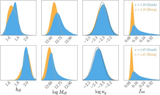
Posterior distribution for the parameters derived from the best-fitting parameters for the Geach (blue) and Zheng (orange) HOD models. From left to right, the posteriors for the effective bias, effective halo mass, galaxy number density, and satellite fraction are shown. The upper and lower panels show the results for z = 1.19 and z = 1.47, respectively. The number density presented here is different from the observed number density shown in table 1 by a factor of (1 − f_fake), |$(1-f_{\rm fake})n_{\rm g}^{\rm obs}$| (see table 3 for the constrained values for f_fake). The Gaussian priors assumed for log n_g are depicted by the black solid curves, where the best-fitting value of f_fake is adopted to multiply by (1 − f_fake). The posterior of log n_g for z = 1.47 (orange) is almost entirely behind the one for z = 1.19. (Color online)

The effective masses of halos hosting [O ii] emitters are derived to be |$\log {M_{\rm eff}/(h^{-1}\, {M}_{\odot })}=12.703^{+0.091}_{-0.069}$| and |$12.609^{+0.085}_{-0.051}$| at z = 1.19 and 1.47, respectively. Figure 11 shows the constraints on M_eff as a function of redshift obtained from our HSC [O ii] emitters, together with the previous studies at 0 < z < 4 which were already presented in Kashino et al. (2017). The constraints include the studies of photo-z galaxies from the CFHT Legacy Survey at z ∼ 0.3, 0.5, and 0.7 (Coupon et al. 2012), the VIMOS-VLT Deep Survey (VVDS) at z ∼ 0.55 and 1 (Abbas et al. 2010), the NEWFIRM Medium Band Survey at z ∼ 1.1 and 1.5 (Wake et al. 2011), Hα emitters from the FMOS-COSMOS Survey at z ∼ 1.6 (Kashino et al. 2017) and from the HiZELS survey at z ∼ 2.2 (Geach et al. 2012), and VUDS at z ∼ 2.5 and 3.5 (Durkalec et al. 2015). These samples have number densities and stellar masses similar to our [O ii] emitter samples. Here we also plot the average mass assembly history of halos with different present-day masses, as derived by Behroozi, Wechsler, and Conroy (2013) based on an N-body simulation. According to this prediction, our measurements of M_eff at two redshifts are well explained by the mass assembly history with M(z = 0) = 1.5 × 10¹³ h⁻¹ M_⊙, as depicted by the blue solid curve. The effective halo mass of [O ii] emitters at z = 1.47 is slightly higher than the blue curve, which reflects the fact that [O ii] emitters of our z = 1.47 sample are intrinsically brighter than those of the lower-z sample (see subsection 2.2). Given the accurate constraints on HOD, one can in principle infer the mass of the host halo for an individual emission line galaxy (Oguri & Lin 2015). It is, however, beyond the scope of this paper and will be investigated in future work.

$Average mass of halos hosting ELGs as a function of redshift. The blue stars are the results from our analysis of [O ii] emitters at z = 1.19 and z = 1.47. The other points are the results of the previous HOD analysis by Abbas et al. (2010), Wake et al. (2011), Geach et al. (2012), Coupon et al. (2012), Durkalec et al. (2015), and Kashino et al. (2017) (see the legend). The solid curves show a prediction of mass accretion histories for halos with M(z = 0) = 1015, 1014, 1013, and 1012 $M_{\odot} $ from top to bottom (Behroozi et al. 2013). The blue curve represents the one with M(z = 0) = 1.5 × 1013 [h−1 $M_{\odot} $]. (Color online)$

Fig. 11.

Average mass of halos hosting ELGs as a function of redshift. The blue stars are the results from our analysis of [O ii] emitters at z = 1.19 and z = 1.47. The other points are the results of the previous HOD analysis by Abbas et al. (2010), Wake et al. (2011), Geach et al. (2012), Coupon et al. (2012), Durkalec et al. (2015), and Kashino et al. (2017) (see the legend). The solid curves show a prediction of mass accretion histories for halos with M(z = 0) = 10¹⁵, 10¹⁴, 10¹³, and 10¹² |$M_{\odot} $| from top to bottom (Behroozi et al. 2013). The blue curve represents the one with M(z = 0) = 1.5 × 10¹³ [h⁻¹ |$M_{\odot} $|]. (Color online)

For our [O ii] emitter sample, the satellite galaxy fraction is constrained as |$f_{\rm sat}=0.158^{+0.114}_{-0.047}$| and |$0.159^{+0.109}_{-0.049}$| at z = 1.19 and 1.47, respectively. The preceding studies revealed that the satellite galaxy fraction of a given population would depend on the redshift, number density, and stellar mass (Coupon et al. 2012; Guo et al. 2014, 2019). At least over the redshift we studied here, the satellite fraction of [O ii] emitters in our sample does not significantly evolve with redshift. The analysis of Favole et al. (2016) constrained the satellite fraction of ELGs with the host halo mass M ∼ 10¹² h⁻¹ M_⊙ as f_sat = 0.225 ± 0.025. Avila et al. (2020) constrained the value of f_sat for ELGs from the eBOSS survey, and the best-fitting value of their baseline model is f_sat = 0.22, consistent with our measurements. However, their constraints are significantly model dependent, and varying the baseline model changes the best-fitting value over 0.18 ≤ f_sat ≤ 0.70. Moreover, the selection of ELGs in the eBOSS survey is quite different from ours based on the NB. We thus cannot make a quantitative comparison with their result. Guo et al. (2019) further studied the relation among the satellite fraction, stellar mass, and halo mass for ELGs from the eBOSS survey. They showed that the host halo mass of ELGs with f_sat ∼ 0.15 is log M/(h⁻¹ M_⊙) ∼ 12.6 and a strong function of the stellar mass. It provides good agreement with our clustering measurements of [O ii] emitters from the HSC survey.

5.5 Comparison with a simpler HOD

While the Geach HOD model is general and flexible, as a trade-off the HOD parameters are constrained more poorly and more degenerate with each other. Furthermore, it is not clear whether different halo occupation functions provide the same physical interpretation for a measured correlation function. A similar attempt has been made by studying one of the simplest HOD models (Zehavi et al. 2005) in Hong et al. (2019); see their appendix B. Here we investigate whether the predicted correlation function, halo occupation function, and host halo parameters of [O ii] emitters can be different between different HOD models.

To see this, we consider the commonly adopted model of Zheng et al. (2005); see also Zheng, Coil, and Zehavi (2007). The model contains five parameters in total, and the central and satellite HODs are, respectively, given by

$$\begin{eqnarray} && N_{\rm cen}(M) = \frac{1}{2}\left[ 1+ {\rm erf}\left(\frac{\log {M / M_{\rm min}}}{\sigma _{\log {M}}}\right) \right], \end{eqnarray}$$

(34)

$$\begin{eqnarray} && N_{\rm sat}(M) = \frac{1}{2}\left[ 1+ {\rm erf}\left(\frac{\log {M / M_{\rm min}}}{\sigma _{\log {M}}}\right) \right] \left(\frac{M-M_0}{M_1}\right)^{\alpha }, \end{eqnarray}$$

(35)

where M_min is the characteristic mass to host a central galaxy, M₁ is the mass for a halo with a central galaxy to host one satellite, M₀ is the mass scale to truncate satellites, σ_log M is the characteristic transition width, and α is the slope of the power law for the satellite HOD, the same as α in the Geach model. The parameter M₀ is a poorly constrained parameter. In order to make this analysis simpler, we impose a relation between M₀ and M₁ following Conroy, Wechsler, and Kravtsov (2006) (see also Kashino et al. 2017),

$$\begin{equation} \log {M_0} / (h^{-1}\, {M}_{\odot }) = 0.76 \log {M_1}/(h^{-1}\, {M}_{\odot }) + 2.3. \end{equation}$$

(36)

Thus, the number of free parameters in the Zheng HOD model together with the fake line fraction is five, Θ = (M_min, M₁, σ_log M, α, f_fake). As is the case for the analysis with the Geach HOD model, we apply Gaussian priors on α and f_fake as α = 1.00 ± 0.20 and f_fake = 0.140 ± 0.060, and flat priors on the other three parameters. We use data with the same angular separation range as the analysis of the Geach HOD model (subsection 5.3), |$0{_{.}^{\circ}} 0015 < \theta < 1$|°; the degree of freedom is ν = N_bin + 1 − 5 = 10.

The resulting constraints on the HOD parameters of Zheng’s model are shown in figure 12 and summarized in table 4. Overall, the constraints on the Zheng HOD model are tighter than those on the Geach model due to the smaller number of parameters. The posterior distribution of the HOD N(M) is shown as the red dashed curve in figure 8. Interestingly, the two models predict very similar HODs, particularly the central ones, for the observed angular correlation function of the [O ii] emitters. The discrepancy seen at M > 10¹³ h⁻¹ M_⊙ is reasonable because such massive halos are rare as hosts of [O ii] emitters; since the varied range of F_s in the Geach model is 0 ≤ F_s ≤ 1, the larger number of 〈N_sat〉 is allowed in the model (see the factor of 1/2 in the Zheng model). Furthermore, since the Zheng model has 〈N_cen〉 = 1 at the high-mass end, it would make sense for the Zheng model to have the lower number of 〈N_sat〉 when the total number density is fixed. Nevertheless, the two N(M) are consistent with each other within 2 σ. The best-fitting correlation function is shown as the red dashed curve in the upper and lower panels of figure 9 for z = 1.19 and z = 1.47, respectively. As expected, the overall shape of the correlation function is very similar to that of the Geach model depicted by the red solid curve. However, one can see that the Geach model shows a better fit to the measured w(θ) at the smallest scales, which would imply that the ELGs in our sample prefer the HOD model which allows massive halos to have no central ELG.

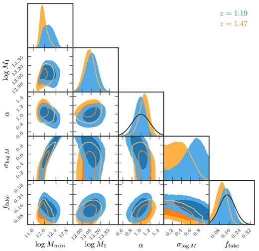
$Constraints on HOD parameters of Zheng’s model, (log Mc, log Mmin, α, σlog M) and ffake, for z = 1.19 (blue) and z = 1.47 (orange). The contours show the $68\%$ and $95\%$ confidence levels. The diagonal panels show the posterior probability distribution of each parameter. Gaussian priors are assumed for α and ffake, as depicted by the black curves in the panels of the one-dimensional posterior distributions. (Color online)$

Fig. 12.

Constraints on HOD parameters of Zheng’s model, (log M_c, log M_min, α, σ_log M) and f_fake, for z = 1.19 (blue) and z = 1.47 (orange). The contours show the |$68\%$| and |$95\%$| confidence levels. The diagonal panels show the posterior probability distribution of each parameter. Gaussian priors are assumed for α and f_fake, as depicted by the black curves in the panels of the one-dimensional posterior distributions. (Color online)

Table 4.

Priors and constraints of the HOD parameters for the Zheng model.*

		NB816		NB921
		Best fit	Posterior PDF	Best fit	Posterior PDF
Parameter	Prior
log M_min/(h⁻¹ M_⊙)	None	12.16	\|$12.14^{+0.19}_{-0.18}$\|	11.88	\|$11.95^{+0.15}_{-0.10}$\|
log M₁/(h⁻¹ M_⊙)	None	13.070	\|$13.062^{+0.084}_{-0.090}$\|	13.000	\|$13.017^{+0.075}_{-0.078}$\|
σ_log M	[0,1]	0.68	\|$0.65^{+0.21}_{-0.32}$\|	0.18	\|$0.34^{+ 0.25}_{- 0.23}$\|
α	1.00 ± 0.20	0.99	\|$0.98^{+0.11}_{-0.12}$\|	1.11	\|$1.07^{+ 0.10}_{- 0.11}$\|
f_fake	0.140 ± 0.060	0.123	\|$0.133^{+0.048}_{-0.048}$\|	0.115	\|$0.098^{+ 0.041}_{- 0.043}$\|
χ²/ν (ν = 10)		1.86		1.42
Inferred quantity	Measurement
log n_g/(h⁻¹ Mpc)⁻³	−2.259 ± 0.068 (NB816)	−2.327	\|$-2.325^{+0.075}_{-0.073}$\|	−2.369	\|$-2.379^{+ 0.075}_{- 0.074}$\|
	−2.344 ± 0.070 (NB921)
f_sat	—	0.100	\|$0.102^{+0.013}_{-0.012}$\|	0.098	\|$0.094^{ + 0.012}_{ - 0.011}$\|
b_eff	—	1.659	\|$1.668^{+0.102}_{-0.089}$\|	2.034	\|$1.983^{+0.077}_{-0.095}$\|
log M_eff/(h⁻¹ M_⊙)	—	12.645	\|$12.647^{+0.052}_{-0.050}$\|	12.591	\|$12.567^{+0.043}_{-0.046}$\|

		NB816		NB921
		Best fit	Posterior PDF	Best fit	Posterior PDF
Parameter	Prior
log M_min/(h⁻¹ M_⊙)	None	12.16	\|$12.14^{+0.19}_{-0.18}$\|	11.88	\|$11.95^{+0.15}_{-0.10}$\|
log M₁/(h⁻¹ M_⊙)	None	13.070	\|$13.062^{+0.084}_{-0.090}$\|	13.000	\|$13.017^{+0.075}_{-0.078}$\|
σ_log M	[0,1]	0.68	\|$0.65^{+0.21}_{-0.32}$\|	0.18	\|$0.34^{+ 0.25}_{- 0.23}$\|
α	1.00 ± 0.20	0.99	\|$0.98^{+0.11}_{-0.12}$\|	1.11	\|$1.07^{+ 0.10}_{- 0.11}$\|
f_fake	0.140 ± 0.060	0.123	\|$0.133^{+0.048}_{-0.048}$\|	0.115	\|$0.098^{+ 0.041}_{- 0.043}$\|
χ²/ν (ν = 10)		1.86		1.42
Inferred quantity	Measurement
log n_g/(h⁻¹ Mpc)⁻³	−2.259 ± 0.068 (NB816)	−2.327	\|$-2.325^{+0.075}_{-0.073}$\|	−2.369	\|$-2.379^{+ 0.075}_{- 0.074}$\|
	−2.344 ± 0.070 (NB921)
f_sat	—	0.100	\|$0.102^{+0.013}_{-0.012}$\|	0.098	\|$0.094^{ + 0.012}_{ - 0.011}$\|
b_eff	—	1.659	\|$1.668^{+0.102}_{-0.089}$\|	2.034	\|$1.983^{+0.077}_{-0.095}$\|
log M_eff/(h⁻¹ M_⊙)	—	12.645	\|$12.647^{+0.052}_{-0.050}$\|	12.591	\|$12.567^{+0.043}_{-0.046}$\|

*

In the “Prior” column the ranges specified in brackets are for uniform priors while for the others we quote the mean and standard deviation of the Gaussian priors. The “Best fit” column shows the parameter set which gives the minimum value of χ². In the “Posterior PDF” column the central value is a median and the error means the 16th–84th percentiles after other parameters are marginalized over. The measured number density log n_g includes non-[O ii] emitters, and thus its best-fitting values differ from the measure ones by log (1 − f_fake) ∼ −0.06.

Table 4.

Priors and constraints of the HOD parameters for the Zheng model.*

		NB816		NB921
		Best fit	Posterior PDF	Best fit	Posterior PDF
Parameter	Prior
log M_min/(h⁻¹ M_⊙)	None	12.16	\|$12.14^{+0.19}_{-0.18}$\|	11.88	\|$11.95^{+0.15}_{-0.10}$\|
log M₁/(h⁻¹ M_⊙)	None	13.070	\|$13.062^{+0.084}_{-0.090}$\|	13.000	\|$13.017^{+0.075}_{-0.078}$\|
σ_log M	[0,1]	0.68	\|$0.65^{+0.21}_{-0.32}$\|	0.18	\|$0.34^{+ 0.25}_{- 0.23}$\|
α	1.00 ± 0.20	0.99	\|$0.98^{+0.11}_{-0.12}$\|	1.11	\|$1.07^{+ 0.10}_{- 0.11}$\|
f_fake	0.140 ± 0.060	0.123	\|$0.133^{+0.048}_{-0.048}$\|	0.115	\|$0.098^{+ 0.041}_{- 0.043}$\|
χ²/ν (ν = 10)		1.86		1.42
Inferred quantity	Measurement
log n_g/(h⁻¹ Mpc)⁻³	−2.259 ± 0.068 (NB816)	−2.327	\|$-2.325^{+0.075}_{-0.073}$\|	−2.369	\|$-2.379^{+ 0.075}_{- 0.074}$\|
	−2.344 ± 0.070 (NB921)
f_sat	—	0.100	\|$0.102^{+0.013}_{-0.012}$\|	0.098	\|$0.094^{ + 0.012}_{ - 0.011}$\|
b_eff	—	1.659	\|$1.668^{+0.102}_{-0.089}$\|	2.034	\|$1.983^{+0.077}_{-0.095}$\|
log M_eff/(h⁻¹ M_⊙)	—	12.645	\|$12.647^{+0.052}_{-0.050}$\|	12.591	\|$12.567^{+0.043}_{-0.046}$\|

		NB816		NB921
		Best fit	Posterior PDF	Best fit	Posterior PDF
Parameter	Prior
log M_min/(h⁻¹ M_⊙)	None	12.16	\|$12.14^{+0.19}_{-0.18}$\|	11.88	\|$11.95^{+0.15}_{-0.10}$\|
log M₁/(h⁻¹ M_⊙)	None	13.070	\|$13.062^{+0.084}_{-0.090}$\|	13.000	\|$13.017^{+0.075}_{-0.078}$\|
σ_log M	[0,1]	0.68	\|$0.65^{+0.21}_{-0.32}$\|	0.18	\|$0.34^{+ 0.25}_{- 0.23}$\|
α	1.00 ± 0.20	0.99	\|$0.98^{+0.11}_{-0.12}$\|	1.11	\|$1.07^{+ 0.10}_{- 0.11}$\|
f_fake	0.140 ± 0.060	0.123	\|$0.133^{+0.048}_{-0.048}$\|	0.115	\|$0.098^{+ 0.041}_{- 0.043}$\|
χ²/ν (ν = 10)		1.86		1.42
Inferred quantity	Measurement
log n_g/(h⁻¹ Mpc)⁻³	−2.259 ± 0.068 (NB816)	−2.327	\|$-2.325^{+0.075}_{-0.073}$\|	−2.369	\|$-2.379^{+ 0.075}_{- 0.074}$\|
	−2.344 ± 0.070 (NB921)
f_sat	—	0.100	\|$0.102^{+0.013}_{-0.012}$\|	0.098	\|$0.094^{ + 0.012}_{ - 0.011}$\|
b_eff	—	1.659	\|$1.668^{+0.102}_{-0.089}$\|	2.034	\|$1.983^{+0.077}_{-0.095}$\|
log M_eff/(h⁻¹ M_⊙)	—	12.645	\|$12.647^{+0.052}_{-0.050}$\|	12.591	\|$12.567^{+0.043}_{-0.046}$\|

*

In the “Prior” column the ranges specified in brackets are for uniform priors while for the others we quote the mean and standard deviation of the Gaussian priors. The “Best fit” column shows the parameter set which gives the minimum value of χ². In the “Posterior PDF” column the central value is a median and the error means the 16th–84th percentiles after other parameters are marginalized over. The measured number density log n_g includes non-[O ii] emitters, and thus its best-fitting values differ from the measure ones by log (1 − f_fake) ∼ −0.06.

The posterior distribution of the derived physical parameters is shown by the function colored orange in figure 10. Since the number density is primarily constrained by our prior, the two models predict the same values. We find that the effective bias b_eff and halo mass log M_eff determined from the Zheng HOD model are also consistent with those from the Geach model within the statistical uncertainties. On the other hand, the satellite fraction is derived to be |$f_{\rm sat} =0.102^{+0.013}_{-0.012}$| and |$0.093^{+0.012}_{-0.011}$| at z = 1.19 and 1.47, respectively. These values are slightly lower than those determined based on the Geach HOD model, respectively |$0.158^{+0.114}_{-0.047}$| and |$0.159^{+0.109}_{-0.049}$|⁠, though the differences are not significant. This again reflects the fact that the Geach model adopts a more flexible parameterization and the larger amplitude of 〈N_sat〉 is allowed. Hence, the one-dimensional posterior of f_sat obtained from the Geach model has a long tail toward the high-f_sat end.

Overall, the differences in the halo parameters for [O ii] emitters determined from the Geach and Zheng HOD models are not significant compared to the current statistical uncertainties. However, such small differences need to be carefully treated in future clustering analysis for ELGs from large galaxy surveys such as the Subaru PFS, DESI, and Euclid surveys.

6 Summary

In this paper we have studied the clustering of emission line galaxies at z > 1 and the physical properties of the dark matter halos which host them. For this purpose we used [O ii] emitters detected at z = 1.19 and 1.47 using two narrow-band filters, NB816 and NB921, respectively, in the Subaru HSC survey (Hayashi et al. 2020). We then measured the angular correlation functions of 8302 (z = 1.19) and 9578 (z = 1.47) [O ii] emitters. Using a simple model of the non-linear correlation function with a linear galaxy bias factor, we measured the bias of [O ii] emitters as |$b=1.61^{+0.13}_{-0.11}$| and |$2.09^{+0.17}_{-0.15}$| at z = 1.19 and 1.47, respectively. We also found that the bias monotonically increases with the line luminosity.

We, for the first time, performed a HOD analysis for the measured correlation functions of [O ii] emitters based on a model developed to describe the population of galaxies selected by star-forming rate (Geach et al. 2012). We varied eight parameters simultaneously with only a few priors. Nevertheless, the two HOD parameters related to the host halo mass have been well constrained given the large sample from the HSC survey.

Based on the constrained HOD parameters, we have derived parameters which describe properties of the host halos of [O ii] emitters, such as the effective bias, effective halo mass, and satellite fraction. The effective biases are determined as |$b_{\rm eff}=1.701^{+0.083}_{-0.110}$| and |$1.981^{+0.072}_{-0.068}$| at z = 1.19 and 1.47, respectively. They are consistent with the linear bias values determined based on a simple non-linear dark matter model. The effective halo masses and satellite fractions are derived as log M_eff/(h⁻¹ M_⊙) ≃ 12.7 (12.6) and f_sat ≃ 0.16 (0.16) at z = 1.19 (1.47). They are consistent with the results of Guo et al. (2019), who studied the relation among f_sat, M_eff, and the stellar mass using the ELG sample from the eBOSS survey. Furthermore, the determined effective halo masses are in good agreement with previous studies of similar tracers of the mass assembly history with M(z = 0) = 1.5 × 10¹³ h⁻¹ M_⊙.

As stated in section 1, ELGs will be a main tracer in large galaxy surveys at high redshifts. In particular, [O ii] emitters will be targeted by many ongoing/future surveys such as the Subaru PFS survey (Takada et al. 2014). The result presented in this paper is useful to construct a mock catalog for cosmological analysis. The physical properties of halos hosting [O ii] emitters revealed in this paper can also be applicable to the Subaru PFS, DESI, and other forthcoming surveys.

In this analysis, both the shape of the angular correlation function and the number density are constrained by the HOD modeling. However, there is a claim that in three-dimensional analysis the HOD would fail to explain the redshift-space clustering and number density simultaneously (Reid et al. 2014; Saito et al. 2016). To investigate this, we need a spectroscopic survey, which can be done with the PFS, DESI, or Euclid surveys.

The narrow-band data of HSC-SSP PDR2 provide emission lines of not only [O ii] but also Hα and [O iii], ranging from z ∼ 0.4 to z ∼ 1.6 (Hayashi et al. 2020). The redshift evolution of physical properties such as the halo mass for ELGs using these multiple emission lines will be studied in future work.

Acknowledgements

TO thanks the members of the Subaru PFS Cosmology Working Group, particularly Masahiro Takada, Eiichiro Komatsu, and Ryu Makiya, for useful correspondences during the regular telecon. TO is grateful to Shogo Ishikawa for discussions. We also thank the anonymous referee for their careful reading and suggestions. TO acknowledges support from the Ministry of Science and Technology of Taiwan under Grant MOST 109-2112-M-001-027- and the Career Development Award, Academia Sinica (AS-CDA-108-M02) for the period 2019–2023. YTL is grateful for support from the Ministry of Science & Technology of Taiwan under grant MOST 109-2112-M-001-005 and a Career Development Award from Academia Sinica (AS-CDA-106-M01). KO is supported by JSPS Overseas Research Fellowships. This work is based on data collected at Subaru Telescope, which is operated by the National Astronomical Observatory of Japan.

The Hyper Suprime-Cam (HSC) collaboration includes the astronomical communities of Japan and Taiwan, and Princeton University. The HSC instrumentation and software were developed by the National Astronomical Observatory of Japan (NAOJ), the Kavli Institute for the Physics and Mathematics of the Universe (Kavli IPMU), the University of Tokyo, the High Energy Accelerator Research Organization (KEK), the Academia Sinica Institute for Astronomy and Astrophysics in Taiwan (ASIAA), and Princeton University. Funding was contributed by the FIRST program from the Japanese Cabinet Office, the Ministry of Education, Culture, Sports, Science and Technology (MEXT), the Japan Society for the Promotion of Science (JSPS), Japan Science and Technology Agency (JST), the Toray Science Foundation, NAOJ, Kavli IPMU, KEK, ASIAA, and Princeton University.

Appendix 1 Correlation functions in individual fields

In order to confirm the consistency of the angular correlation functions among different fields, we present the measurements from each of the individual four fields, |$\hat{w}_k$|⁠, as the black points in figure 13. The square roots of the diagonal components of the covariance matrix, |$C_{k,ii}^{1/2}$|⁠, are shown as the error bars. The results for z = 1.19 and z = 1.47 are shown in the upper and lower panels, respectively. In order to compare the correlation functions between different fields, we need to take into account the correction of the integral constraint because the survey volume of each field is different. To estimate the integral constraint for the kth field, w_Ω,k, the random–random count for the field, RR_k, is used as RR in equation (11), and

$$\begin{equation} w_{\Omega ,k}(\Theta ) = \frac{\sum _i{w(\theta _i;\Theta )RR_k(\theta _i)}}{\sum _i{RR_k(\theta _i)}}. \end{equation}$$

(A1)

For w(θ_i; Θ) in equation (A1), we use the best-fitting linearly biased dark matter model for the combined field obtained in subsection 4.3, (b, f_fake) = (1.60, 0.140) for z = 1.19 and (b, f_fake) = (2.08, 0.140) for z = 1.47. The red points show the result with the integral constraint correction, |$\hat{w}_k+(1-f_{\rm fake})^2 w_\Omega$|⁠. For comparison, the measurement from all four fields with the integral constraint calculated using the same model is plotted as the blue dashed curve. One can see that the measurements from each field are largely consistent with each other. Thus, throughout this paper we perform the statistical analysis only for the data combined over all four fields.

$Angular correlation functions of [O ii] emitters of each of the four fields measured at z = 1.19 (top) and z = 1.47 (bottom). In each column, the measurement from each of the individual four fields is presented. The black points are the raw measurement without the correction of the integral constraints, $\hat{w}_k$ (1 ≤ k ≤ 4). The red points are after the integral constraint (denoted by IC in the legend) is taken into account with the linearly biased dark matter model, $\hat{w}_k+(1-f_{\rm fake})^2w_{\Omega ,k}$, with the best-fitting parameters obtained for the combined field, (b, ffake) = (1.60, 0.140) (z = 1.19) and (b, ffake) = (2.08, 0.140) (z = 1.47). For reference, the angular correlation function measured for the combined field, $\hat{w}+(1-f_{\rm fake})^2w_\Omega$, is shown as the blue dashed curve. (Color online)$

Fig. 13.

Angular correlation functions of [O ii] emitters of each of the four fields measured at z = 1.19 (top) and z = 1.47 (bottom). In each column, the measurement from each of the individual four fields is presented. The black points are the raw measurement without the correction of the integral constraints, |$\hat{w}_k$| (1 ≤ k ≤ 4). The red points are after the integral constraint (denoted by IC in the legend) is taken into account with the linearly biased dark matter model, |$\hat{w}_k+(1-f_{\rm fake})^2w_{\Omega ,k}$|⁠, with the best-fitting parameters obtained for the combined field, (b, f_fake) = (1.60, 0.140) (z = 1.19) and (b, f_fake) = (2.08, 0.140) (z = 1.47). For reference, the angular correlation function measured for the combined field, |$\hat{w}+(1-f_{\rm fake})^2w_\Omega$|⁠, is shown as the blue dashed curve. (Color online)

Appendix 2 Constraints on HOD parameters using clustering only

Given a HOD model for a certain galaxy population, the average number density is calculated by equation (21). One therefore needs to simultaneously analyze the observed correlation function and the number density to constrain the HOD model, as performed in subsection 5.3. In this appendix, we present the constraints on the HOD parameters based on the Geach and Zheng models without using the information of the measured number density of [O ii] emitters for readers who are interested in the constraining power coming from the clustering only; see, e.g., Matsuoka et al. (2011) and Martinez-Manso et al. (2015) for similar attempts.

Table 5 shows these results without using the abundance information. The halo mass parameters are strongly constrained by the abundance of [O ii] emitters. The constraints on these parameters are thus not as tight as those presented in tables 3 and 4, as expected: the errors on the M_c and M_min constraints without the abundance information in the Geach model are ∼1.5 and ∼3 times larger than those with the simultaneous analysis of clustering and abundance, and the errors on the M_min and M₁ constraints without the abundance information in the Zheng model are ∼3 and ∼4 times larger. There are no significant changes in the constraints of the other HOD parameters. Interestingly, even though we do not use the number density to constrain the HOD parameters, the posterior of the number density is consistent with the observed one.

Table 5.

Priors and constraints of the HOD parameters for the Geach and Zheng models obtained using the clustering information only.*

		NB816	NB921
		Posterior PDF	Posterior PDF
Geach HOD model
Parameter	Prior
log M_c/(h⁻¹ M_⊙)	None	\|$11.50^{+0.72}_{-0.28}$\|	\|$11.70^{+ 0.25} _{- 0.20}$\|
log M_min/(h⁻¹ M_⊙)	None	\|$11.40^{+1.25}_{-1.00}$\|	\|$11.89^{+0.76}_{-1.36}$\|
σ_log M	[0,1]	\|$0.27^{+0.33}_{-0.17}$\|	\|$0.22^{+ 0.16}_{- 0.13}$\|
α	1.00 ± 0.20	\|$0.96^{+0.11}_{-0.09}$\|	\|$1.10^{+ 0.13}_{- 0.13}$\|
\|$F_c^A$\|	[0, 0.5]	\|$0.22^{+0.14}_{-0.07}$\|	\|$0.17^{+ 0.18}_{- 0.06}$\|
\|$F_c^B$\|	[0,1]	\|$0.56^{+0.32}_{-0.39}$\|	\|$0.61^{+ 0.27}_{- 0.34}$\|
F_s	[0, 1]	\|$0.54^{+0.32}_{-0.30}$\|	\|$0.52^{+ 0.32}_{- 0.34}$\|
f_fake	0.140 ± 0.060	\|$0.124^{+0.054}_{-0.051}$\|	\|$0.091^{+ 0.054}_{- 0.046}$\|
Inferred quantity	Measurement
log n_g/(h⁻¹ Mpc)⁻³	—	\|$-1.47^{+0.89}_{-0.80}$\|	\|$-1.96^{+1.18}_{-0.42}$\|
f_sat	—	\|$0.58^{+0.33}_{-0.43}$\|	\|$0.38^{ + 0.54}_{ - 0.23}$\|
b_eff	—	\|$1.64^{+0.12}_{-0.10}$\|	\|$1.94^{+0.13}_{-0.11}$\|
log M_eff/(h⁻¹ M_⊙)	—	\|$12.70^{+0.10}_{-0.09}$\|	\|$12.63^{+0.12}_{-0.10}$\|
Zheng HOD model
Parameter	Prior
log M_min/(h⁻¹ M_⊙)	None	\|$12.01^{+0.62}_{-0.61}$\|	\|$11.85^{+ 0.56}_{-0.26}$\|
log M₁/(h⁻¹ M_⊙)	None	\|$12.97^{+0.43}_{-0.64}$\|	\|$12.91^{+0.36}_{-0.31}$\|
σ_log M	[0,1]	\|$0.58^{+0.30}_{-0.41}$\|	\|$0.32^{+0.41}_{-0.22}$\|
α	1.00 ± 0.20	\|$0.94^{+0.11}_{-0.11}$\|	\|$1.02^{+0.11}_{-0.11}$\|
f_fake	0.140 ± 0.060	\|$0.123^{+0.060}_{-0.063}$\|	\|$0.077^{+ 0.055}_{- 0.047}$\|
Inferred quantity	Measurement
log n_g/(h⁻¹ Mpc)⁻³	—	\|$-2.24^{+0.56}_{- 0.44}$\|	\|$-2.27^{+0.28}_{-0.38}$\|
f_sat	—	\|$0.113^{+0.100}_{-0.044}$\|	\|$0.106^{+ 0.047}_{-0.040}$\|
b_eff	—	\|$1.64^{+ 0.15}_{-0.15}$\|	\|$1.91^{+0.13}_{-0.11}$\|
log M_eff/(h⁻¹ M_⊙)	—	\|$12.633^{+0.102}_{-0.107}$\|	\|$12.534^{+0.091}_{-0.077}$\|

		NB816	NB921
		Posterior PDF	Posterior PDF
Geach HOD model
Parameter	Prior
log M_c/(h⁻¹ M_⊙)	None	\|$11.50^{+0.72}_{-0.28}$\|	\|$11.70^{+ 0.25} _{- 0.20}$\|
log M_min/(h⁻¹ M_⊙)	None	\|$11.40^{+1.25}_{-1.00}$\|	\|$11.89^{+0.76}_{-1.36}$\|
σ_log M	[0,1]	\|$0.27^{+0.33}_{-0.17}$\|	\|$0.22^{+ 0.16}_{- 0.13}$\|
α	1.00 ± 0.20	\|$0.96^{+0.11}_{-0.09}$\|	\|$1.10^{+ 0.13}_{- 0.13}$\|
\|$F_c^A$\|	[0, 0.5]	\|$0.22^{+0.14}_{-0.07}$\|	\|$0.17^{+ 0.18}_{- 0.06}$\|
\|$F_c^B$\|	[0,1]	\|$0.56^{+0.32}_{-0.39}$\|	\|$0.61^{+ 0.27}_{- 0.34}$\|
F_s	[0, 1]	\|$0.54^{+0.32}_{-0.30}$\|	\|$0.52^{+ 0.32}_{- 0.34}$\|
f_fake	0.140 ± 0.060	\|$0.124^{+0.054}_{-0.051}$\|	\|$0.091^{+ 0.054}_{- 0.046}$\|
Inferred quantity	Measurement
log n_g/(h⁻¹ Mpc)⁻³	—	\|$-1.47^{+0.89}_{-0.80}$\|	\|$-1.96^{+1.18}_{-0.42}$\|
f_sat	—	\|$0.58^{+0.33}_{-0.43}$\|	\|$0.38^{ + 0.54}_{ - 0.23}$\|
b_eff	—	\|$1.64^{+0.12}_{-0.10}$\|	\|$1.94^{+0.13}_{-0.11}$\|
log M_eff/(h⁻¹ M_⊙)	—	\|$12.70^{+0.10}_{-0.09}$\|	\|$12.63^{+0.12}_{-0.10}$\|
Zheng HOD model
Parameter	Prior
log M_min/(h⁻¹ M_⊙)	None	\|$12.01^{+0.62}_{-0.61}$\|	\|$11.85^{+ 0.56}_{-0.26}$\|
log M₁/(h⁻¹ M_⊙)	None	\|$12.97^{+0.43}_{-0.64}$\|	\|$12.91^{+0.36}_{-0.31}$\|
σ_log M	[0,1]	\|$0.58^{+0.30}_{-0.41}$\|	\|$0.32^{+0.41}_{-0.22}$\|
α	1.00 ± 0.20	\|$0.94^{+0.11}_{-0.11}$\|	\|$1.02^{+0.11}_{-0.11}$\|
f_fake	0.140 ± 0.060	\|$0.123^{+0.060}_{-0.063}$\|	\|$0.077^{+ 0.055}_{- 0.047}$\|
Inferred quantity	Measurement
log n_g/(h⁻¹ Mpc)⁻³	—	\|$-2.24^{+0.56}_{- 0.44}$\|	\|$-2.27^{+0.28}_{-0.38}$\|
f_sat	—	\|$0.113^{+0.100}_{-0.044}$\|	\|$0.106^{+ 0.047}_{-0.040}$\|
b_eff	—	\|$1.64^{+ 0.15}_{-0.15}$\|	\|$1.91^{+0.13}_{-0.11}$\|
log M_eff/(h⁻¹ M_⊙)	—	\|$12.633^{+0.102}_{-0.107}$\|	\|$12.534^{+0.091}_{-0.077}$\|

*

In the “Prior” column the ranges specified in brackets are for uniform priors while for the others we quote the mean and standard deviation of the Gaussian priors. In the “Posterior PDF” column the central value is a median and the error means the 16th–84th percentiles after other parameters are marginalized over.

Table 5.

〈https://subarutelescope.org/Observing/Instruments/HSC/sensitivity.html〉.

Priors and constraints of the HOD parameters for the Geach and Zheng models obtained using the clustering information only.*

		NB816	NB921
		Posterior PDF	Posterior PDF
Geach HOD model
Parameter	Prior
log M_c/(h⁻¹ M_⊙)	None	\|$11.50^{+0.72}_{-0.28}$\|	\|$11.70^{+ 0.25} _{- 0.20}$\|
log M_min/(h⁻¹ M_⊙)	None	\|$11.40^{+1.25}_{-1.00}$\|	\|$11.89^{+0.76}_{-1.36}$\|
σ_log M	[0,1]	\|$0.27^{+0.33}_{-0.17}$\|	\|$0.22^{+ 0.16}_{- 0.13}$\|
α	1.00 ± 0.20	\|$0.96^{+0.11}_{-0.09}$\|	\|$1.10^{+ 0.13}_{- 0.13}$\|
\|$F_c^A$\|	[0, 0.5]	\|$0.22^{+0.14}_{-0.07}$\|	\|$0.17^{+ 0.18}_{- 0.06}$\|
\|$F_c^B$\|	[0,1]	\|$0.56^{+0.32}_{-0.39}$\|	\|$0.61^{+ 0.27}_{- 0.34}$\|
F_s	[0, 1]	\|$0.54^{+0.32}_{-0.30}$\|	\|$0.52^{+ 0.32}_{- 0.34}$\|
f_fake	0.140 ± 0.060	\|$0.124^{+0.054}_{-0.051}$\|	\|$0.091^{+ 0.054}_{- 0.046}$\|
Inferred quantity	Measurement
log n_g/(h⁻¹ Mpc)⁻³	—	\|$-1.47^{+0.89}_{-0.80}$\|	\|$-1.96^{+1.18}_{-0.42}$\|
f_sat	—	\|$0.58^{+0.33}_{-0.43}$\|	\|$0.38^{ + 0.54}_{ - 0.23}$\|
b_eff	—	\|$1.64^{+0.12}_{-0.10}$\|	\|$1.94^{+0.13}_{-0.11}$\|
log M_eff/(h⁻¹ M_⊙)	—	\|$12.70^{+0.10}_{-0.09}$\|	\|$12.63^{+0.12}_{-0.10}$\|
Zheng HOD model
Parameter	Prior
log M_min/(h⁻¹ M_⊙)	None	\|$12.01^{+0.62}_{-0.61}$\|	\|$11.85^{+ 0.56}_{-0.26}$\|
log M₁/(h⁻¹ M_⊙)	None	\|$12.97^{+0.43}_{-0.64}$\|	\|$12.91^{+0.36}_{-0.31}$\|
σ_log M	[0,1]	\|$0.58^{+0.30}_{-0.41}$\|	\|$0.32^{+0.41}_{-0.22}$\|
α	1.00 ± 0.20	\|$0.94^{+0.11}_{-0.11}$\|	\|$1.02^{+0.11}_{-0.11}$\|
f_fake	0.140 ± 0.060	\|$0.123^{+0.060}_{-0.063}$\|	\|$0.077^{+ 0.055}_{- 0.047}$\|
Inferred quantity	Measurement
log n_g/(h⁻¹ Mpc)⁻³	—	\|$-2.24^{+0.56}_{- 0.44}$\|	\|$-2.27^{+0.28}_{-0.38}$\|
f_sat	—	\|$0.113^{+0.100}_{-0.044}$\|	\|$0.106^{+ 0.047}_{-0.040}$\|
b_eff	—	\|$1.64^{+ 0.15}_{-0.15}$\|	\|$1.91^{+0.13}_{-0.11}$\|
log M_eff/(h⁻¹ M_⊙)	—	\|$12.633^{+0.102}_{-0.107}$\|	\|$12.534^{+0.091}_{-0.077}$\|

		NB816	NB921
		Posterior PDF	Posterior PDF
Geach HOD model
Parameter	Prior
log M_c/(h⁻¹ M_⊙)	None	\|$11.50^{+0.72}_{-0.28}$\|	\|$11.70^{+ 0.25} _{- 0.20}$\|
log M_min/(h⁻¹ M_⊙)	None	\|$11.40^{+1.25}_{-1.00}$\|	\|$11.89^{+0.76}_{-1.36}$\|
σ_log M	[0,1]	\|$0.27^{+0.33}_{-0.17}$\|	\|$0.22^{+ 0.16}_{- 0.13}$\|
α	1.00 ± 0.20	\|$0.96^{+0.11}_{-0.09}$\|	\|$1.10^{+ 0.13}_{- 0.13}$\|
\|$F_c^A$\|	[0, 0.5]	\|$0.22^{+0.14}_{-0.07}$\|	\|$0.17^{+ 0.18}_{- 0.06}$\|
\|$F_c^B$\|	[0,1]	\|$0.56^{+0.32}_{-0.39}$\|	\|$0.61^{+ 0.27}_{- 0.34}$\|
F_s	[0, 1]	\|$0.54^{+0.32}_{-0.30}$\|	\|$0.52^{+ 0.32}_{- 0.34}$\|
f_fake	0.140 ± 0.060	\|$0.124^{+0.054}_{-0.051}$\|	\|$0.091^{+ 0.054}_{- 0.046}$\|
Inferred quantity	Measurement
log n_g/(h⁻¹ Mpc)⁻³	—	\|$-1.47^{+0.89}_{-0.80}$\|	\|$-1.96^{+1.18}_{-0.42}$\|
f_sat	—	\|$0.58^{+0.33}_{-0.43}$\|	\|$0.38^{ + 0.54}_{ - 0.23}$\|
b_eff	—	\|$1.64^{+0.12}_{-0.10}$\|	\|$1.94^{+0.13}_{-0.11}$\|
log M_eff/(h⁻¹ M_⊙)	—	\|$12.70^{+0.10}_{-0.09}$\|	\|$12.63^{+0.12}_{-0.10}$\|
Zheng HOD model
Parameter	Prior
log M_min/(h⁻¹ M_⊙)	None	\|$12.01^{+0.62}_{-0.61}$\|	\|$11.85^{+ 0.56}_{-0.26}$\|
log M₁/(h⁻¹ M_⊙)	None	\|$12.97^{+0.43}_{-0.64}$\|	\|$12.91^{+0.36}_{-0.31}$\|
σ_log M	[0,1]	\|$0.58^{+0.30}_{-0.41}$\|	\|$0.32^{+0.41}_{-0.22}$\|
α	1.00 ± 0.20	\|$0.94^{+0.11}_{-0.11}$\|	\|$1.02^{+0.11}_{-0.11}$\|
f_fake	0.140 ± 0.060	\|$0.123^{+0.060}_{-0.063}$\|	\|$0.077^{+ 0.055}_{- 0.047}$\|
Inferred quantity	Measurement
log n_g/(h⁻¹ Mpc)⁻³	—	\|$-2.24^{+0.56}_{- 0.44}$\|	\|$-2.27^{+0.28}_{-0.38}$\|
f_sat	—	\|$0.113^{+0.100}_{-0.044}$\|	\|$0.106^{+ 0.047}_{-0.040}$\|
b_eff	—	\|$1.64^{+ 0.15}_{-0.15}$\|	\|$1.91^{+0.13}_{-0.11}$\|
log M_eff/(h⁻¹ M_⊙)	—	\|$12.633^{+0.102}_{-0.107}$\|	\|$12.534^{+0.091}_{-0.077}$\|

*

In the “Prior” column the ranges specified in brackets are for uniform priors while for the others we quote the mean and standard deviation of the Gaussian priors. In the “Posterior PDF” column the central value is a median and the error means the 16th–84th percentiles after other parameters are marginalized over.

Footnotes

1

We use a composite model magnitude named cmodel.

2

〈https://github.com/esheldon/kmeans_radec〉.

3

4

If f_fake becomes large so that the contribution from non-[O ii] emitters is non-negligible, a sophisticated treatment of the line contaminant for the cosmological analysis is required (e.g., Leung et al. 2017; Addison et al. 2019).

5

References

Abbas

U.

et al.

2010

,

MNRAS

,

406

,

1306

Adams

J. J.

et al.

2011

,

ApJS

,

192

,

5

Addison

G. E.

,

Bennett

C. L.

,

Jeong

D.

,

Komatsu

E.

,

Weiland

J. L.

2019

,

ApJ

,

879

,

15

Aihara

H.

et al.

2018a

,

PASJ

,

70

,

S4

Aihara

H.

et al.

2018b

,

PASJ

,

70

,

S8

Aihara

H.

et al.

2019

,

PASJ

,

71

,

114

Avila

S.

et al.

2020

,

MNRAS

,

499

,

5486

Behroozi

P. S.

,

Wechsler

R. H.

,

Conroy

C.

2013

,

ApJ

,

770

,

57

Berlind

A. A.

,

Weinberg

D. H.

2002

,

ApJ

,

575

,

587

Blake

C.

,

Collister

A.

,

Lahav

O.

2008

,

MNRAS

,

385

,

1257

Bocquet

S.

,

Carter

F. W.

2016

,

J. Open Source Software

,

1

,

46

Bosch

J.

et al.

2018

,

PASJ

,

70

,

S5

Bullock

J. S.

,

Wechsler

R. H.

,

Somerville

R. S.

2002

,

MNRAS

,

329

,

246

Cochrane

R. K.

,

Best

P. N.

,

Sobral

D.

,

Smail

I.

,

Geach

J. E.

,

Stott

J. P.

,

Wake

D. A.

2018

,

MNRAS

,

475

,

3730

Cochrane

R. K.

,

Best

P. N.

,

Sobral

D.

,

Smail

I.

,

Wake

D. A.

,

Stott

J. P.

,

Geach

J. E.

2017

,

MNRAS

,

469

,

2913

Comparat

J.

et al.

2016

,

MNRAS

,

461

,

1076

Conroy

C.

,

Wechsler

R. H.

,

Kravtsov

A. V.

2006

,

ApJ

,

647

,

201

Contreras

S.

,

Baugh

C. M.

,

Norberg

P.

,

Padilla

N.

2013

,

MNRAS

,

432

,

2717

Cooray

A.

,

Sheth

R.

2002

,

Phys. Rep.

,

372

,

1

Coupon

J.

et al.

2012

,

A&A

,

542

,

A5

Coupon

J.

,

Czakon

N.

,

Bosch

J.

,

Komiyama

Y.

,

Medezinski

E.

,

Miyazaki

S.

,

Oguri

M.

2018

,

PASJ

,

70

,

S7

Crocce

M.

,

Cabré

A.

,

Gaztañaga

E.

2011

,

MNRAS

,

414

,

329

Dawson

K. S.

et al.

2016

,

AJ

,

151

,

44

de la Torre

S.

et al.

2013

,

A&A

,

557

,

A54

DESI Collaboration

2016

,

arXiv:1611.00036

Doré

O.

et al.

2014

,

arXiv:1412.4872

Duffy

A. R.

,

Schaye

J.

,

Kay

S. T.

,

Dalla Vecchia

C.

2008

,

MNRAS

,

390

,

L64

Durkalec

A.

et al.

2015

,

A&A

,

583

,

A128

Efstathiou

G.

,

Bernstein

G.

,

Katz

N.

,

Tyson

J. A.

,

Guhathakurta

P.

1991

,

ApJL

,

380

,

L47

Favole

G.

et al.

2016

,

MNRAS

,

461

,

3421

Favole

G.

et al.

2020

,

MNRAS

,

497

,

5432

Foreman-Mackey

D.

,

Hogg

D. W.

,

Lang

D.

,

Goodman

J.

2013

,

PASP

,

125

,

306

Furusawa

H.

et al.

2018

,

PASJ

,

70

,

S3

Gao

H.

,

Jing

Y. P.

2021

,

ApJ

,

908

,

43

Geach

J. E.

,

Smail

I.

,

Best

P. N.

,

Kurk

J.

,

Casali

M.

,

Ivison

R. J.

,

Coppin

K.

2008

,

MNRAS

,

388

,

1473

Geach

J. E.

,

Sobral

D.

,

Hickox

R. C.

,

Wake

D. A.

,

Smail

I.

,

Best

P. N.

,

Baugh

C. M.

,

Stott

J. P.

2012

,

MNRAS

,

426

,

679

Gonzalez-Perez

V.

et al.

2018

,

MNRAS

,

474

,

4024

Gonzalez-Perez

V.

et al.

2020

,

MNRAS

,

498

,

1852

Guo

H.

et al.

2014

,

MNRAS

,

441

,

2398

Guo

H.

et al.

2019

,

ApJ

,

871

,

147

Hadzhiyska

B.

,

Tacchella

S.

,

Bose

S.

,

Eisenstein

D. J.

2021

,

MNRAS

,

502

,

3599

Hamana

T.

,

Ouchi

M.

,

Shimasaku

K.

,

Kayo

I.

,

Suto

Y.

2004

,

MNRAS

,

347

,

813

Harikane

Y.

et al.

2016

,

ApJ

,

821

,

123

Harikane

Y.

et al.

2018

,

PASJ

,

70

,

S11

Hartlap

J.

,

Simon

P.

,

Schneider

P.

2007

,

A&A

,

464

,

399

Hayashi

M.

et al.

2015

,

PASJ

,

67

,

80

Hayashi

M.

et al.

2018

,

PASJ

,

70

,

S17

Hayashi

M.

et al.

2020

,

PASJ

,

72

,

86

Hayashi

M.

,

Sobral

D.

,

Best

P. N.

,

Smail

I.

,

Kodama

T.

2013

,

MNRAS

,

430

,

1042

Hikage

C.

,

Mandelbaum

R.

,

Takada

M.

,

Spergel

D. N.

2013

,

MNRAS

,

435

,

2345

Hong

S.

et al.

2019

,

MNRAS

,

483

,

3950

Hsieh

B. C.

,

Yee

H. K. C.

2014

,

ApJ

,

792

,

102

Huang

S.

et al.

2018

,

PASJ

,

70

,

S6

Ishikawa

S.

et al.

2017

,

ApJ

,

841

,

8

Ishikawa

S.

et al.

2020

,

ApJ

,

904

,

128

Jing

Y. P.

,

Mo

H. J.

,

Boerner

G.

1998

,

ApJ

,

494

,

1

Kaiser

N.

1984

,

ApJL

,

284

,

L9

Kashino

D.

et al.

2017

,

ApJ

,

843

,

138

Kayo

I.

,

Oguri

M.

2012

,

MNRAS

,

424

,

1363

Khostovan

A. A.

et al.

2018

,

MNRAS

,

478

,

2999

Kim

H.-S.

,

Baugh

C. M.

,

Benson

A. J.

,

Cole

S.

,

Frenk

C. S.

,

Lacey

C. G.

,

Power

C.

,

Schneider

M.

2011

,

MNRAS

,

414

,

2367

Koda

J.

,

Blake

C.

,

Beutler

F.

,

Kazin

E.

,

Marin

F.

2016

,

MNRAS

,

459

,

2118

Komiyama

Y.

et al.

2018

,

PASJ

,

70

,

S2

Landy

S. D.

,

Szalay

A. S.

1993

,

ApJ

,

412

,

64

Laureijs

R.

et al.

2011

,

arXiv:1110.3193

Leung

A. S.

et al.

2017

,

ApJ

,

843

,

130

Limber

D. N.

1954

,

ApJ

,

119

,

655

Lupton

R.

1993

,

Statistics in Theory and Practice

(

Princeton

:

Princeton University Press

)

Ly

C.

,

Malkan

M. A.

,

Kashikawa

N.

,

Hayashi

M.

,

Nagao

T.

,

Shimasaku

K.

,

Ota

K.

,

Ross

N. R.

2012

,

ApJ

,

757

,

63

Ma

C.-P.

,

Fry

J. N.

2000

,

ApJ

,

543

,

503

Martinez-Manso

J.

,

Gonzalez

A. H.

,

Ashby

M. L. N.

,

Stanford

S. A.

,

Brodwin

M.

,

Holder

G. P.

,

Stern

D.

2015

,

MNRAS

,

446

,

169

Matsuoka

Y.

,

Masaki

S.

,

Kawara

K.

,

Sugiyama

N.

2011

,

MNRAS

,

410

,

548

Miyazaki

S.

et al.

2012

, in

Proc. SPIE, 8446, Ground-based and Airborne Instrumentation for Astronomy IV

, ed.

McLean

I. S.

et al. (

Bellingham, WA

:

SPIE

),

84460Z

Miyazaki

S.

et al.

2018

,

PASJ

,

70

,

S1

Moustakas

L. A.

,

Somerville

R. S.

2002

,

ApJ

,

577

,

1

Murray

S. G.

,

Power

C.

,

Robotham

A. S. G.

2013

,

Astron. Comput.

,

3

,

23

Navarro

J. F.

,

Frenk

C. S.

,

White

S. D. M.

1997

,

ApJ

,

490

,

493

Oguri

M.

,

Lin

Y.-T.

2015

,

ApJ

,

801

,

94

Okada

H.

et al.

2016

,

PASJ

,

68

,

47

Okumura

T.

et al.

2016

,

PASJ

,

68

,

38

Okumura

T.

,

Hand

N.

,

Seljak

U.

,

Vlah

Z.

,

Desjacques

V.

2015

,

Phys. Rev. D

,

92

,

103516

Okumura

T.

,

Takada

M.

,

More

S.

,

Masaki

S.

2017

,

MNRAS

,

469

,

459

Peacock

J. A.

,

Smith

R. E.

2000

,

MNRAS

,

318

,

1144

Peebles

P. J. E.

1973

,

ApJ

,

185

,

413

Peebles

P. J. E.

1980

,

The Large-Scale Structure of the Universe

(

Princeton

:

Princeton University Press

)

Google Scholar

Google Preview

OpenURL Placeholder Text

WorldCat

Peebles

P. J. E.

,

Groth

E. J.

1976

,

A&A

,

53

,

131

Planck Collaboration

2016

,

A&A

,

594

,

A13

Reid

B. A.

,

Seo

H.-J.

,

Leauthaud

A.

,

Tinker

J. L.

,

White

M.

2014

,

MNRAS

,

444

,

476

Richardson

J.

,

Zheng

Z.

,

Chatterjee

S.

,

Nagai

D.

,

Shen

Y.

2012

,

ApJ

,

755

,

30

Saito

S.

,

de la Torre

S.

,

Ilbert

O.

,

Dubois

C.

,

Yabe

K.

,

Coupon

J.

2020

,

MNRAS

,

494

,

199

Saito

S.

et al.

2016

,

MNRAS

,

460

,

1457

Scoccimarro

R.

,

Sheth

R. K.

,

Hui

L.

,

Jain

B.

2001

,

ApJ

,

546

,

20

Seljak

U.

2000

,

MNRAS

,

318

,

203

Simon

P.

2007

,

A&A

,

473

,

711

Takada

M.

et al.

2014

,

PASJ

,

66

,

1

Takahashi

R.

,

Sato

M.

,

Nishimichi

T.

,

Taruya

A.

,

Oguri

M.

2012

,

ApJ

,

761

,

152

Tinker

J. L.

,

Robertson

B. E.

,

Kravtsov

A. V.

,

Klypin

A.

,

Warren

M. S.

,

Yepes

G.

,

Gottlöber

S.

2010

,

ApJ

,

724

,

878

Tonegawa

M.

et al.

2015

,

PASJ

,

67

,

81

Totsuji

H.

,

Kihara

T.

1969

,

PASJ

,

21

,

221

van den Bosch

F. C.

,

More

S.

,

Cacciato

M.

,

Mo

H.

,

Yang

X.

2013

,

MNRAS

,

430

,

725

Wake

D. A.

et al.

2011

,

ApJ

,

728

,

46

Weinberg

D. H.

,

Mortonson

M. J.

,

Eisenstein

D. J.

,

Hirata

C.

,

Riess

A. G.

,

Rozo

E.

2013

,

Phys. Rep.

,

530

,

87

White

M.

et al.

2011

,

ApJ

,

728

,

126

Zehavi

I.

et al.

2005

,

ApJ

,

621

,

22

Zehavi

I.

et al.

2011

,

ApJ

,

736

,

59

Zheng

Z.

et al.

2005

,

ApJ

,

633

,

791

Zheng

Z.

,

Coil

A. L.

,

Zehavi

I.

2007

,

ApJ

,

667

,

760

Zheng

Z.

,

Zehavi

I.

,

Eisenstein

D. J.

,

Weinberg

D. H.

,

Jing

Y. P.

2009

,

ApJ

,

707

,

554