-
PDF
- Split View
-
Views
-
Cite
Cite
Michiko S Fujii, Takayuki R Saitoh, Yutaka Hirai, Long Wang, SIRIUS project. III. Star-by-star simulations of star cluster formation using a direct N-body integrator with stellar feedback, Publications of the Astronomical Society of Japan, Volume 73, Issue 4, August 2021, Pages 1074–1099, https://doi.org/10.1093/pasj/psab061
Close - Share Icon Share
Abstract
One of the computational challenges of cluster formation simulations is resolving individual stars and simulating massive clusters with masses of more than 104 M⊙ without gravitational softening. Combining a direct N-body code with smoothed-particle hydrodynamics (SPH) code, we have developed a new code, ASURA+BRIDGE, in which we can integrate stellar particles without softening. We add a feedback model for H ii regions into this code, in which thermal and momentum feedback is given within the Strömgren radius. We perform N-body/SPH simulations of star cluster formation. Without softening, a portion of massive stars are ejected from the forming clusters. As a result, the stellar feedback works outside the clusters. This enhances/suppresses the star formation in initially sub-virial/super-virial clouds. We find that the formed star clusters are denser than currently observed open clusters, but the mass–density relation is consistent with or even higher than that which is estimated as an initial cluster density. We also find that some clusters have multiple peaks in their stellar age distribution as a consequence of their hierarchical formation. Irrespective of the virial ratio of molecular clouds, approximately one-third of stars remain in the star clusters after gas expulsion.
1 Introduction
Most stars form in star clusters (Lada & Lada 2003). The formation process of star clusters is closely related to the formation of massive stars. Once massive stars have formed in star clusters, they ionize the surrounding gas, their stellar wind blows out the gas, and finally, supernovae eject all the remaining gas (Rauw et al. 2007; Longmore et al. 2014; Krumholz et al. 2019, and references therein). Such gas expulsion processes are also important for understanding the initial states of observed star clusters and their later dynamical evolution (Pfalzner et al. 2014; Farias et al. 2015; Haghi et al. 2015).
To obtain the dynamical evolution of star clusters as collisional systems, we need to integrate the stellar systems without gravitational softening, i.e., we need a direct N-body integration of stars. In previous studies based on direct N-body simulations, fixed potential for the gas distribution was assumed as background gas distribution (Pfalzner et al. 2014; Farias et al. 2015; Haghi et al. 2015). Spherical potential is usually assumed in such simulations. In contrast, observations of actual star-cluster-forming regions imply hierarchical formation of star clusters in turbulent molecular clouds (Gutermuth et al. 2005; Sabbi et al. 2012; Longmore et al. 2014; Zeidler et al. 2015).
Simulations of star-cluster formation originating from turbulent molecular clouds have been dramatically improved in the last 20 years. In pioneering work by Bonnell, Bate, and Vine (2003) using a smoothed-particle hydrodynamics (SPH) method (Lucy 1977; Gingold & Monaghan 1977) with a sink method (Bate et al. 1995), hierarchical formation of star clusters was demonstrated. These types of simulations have improved resolution and include radiation feedback from stars. The maximum total stellar mass in the models used by Dale, Ercolano, and Clarke (2007) and Dale, Ercolano, and Bonnell (2012) was 1000 M⊙. Although this is close to the typical mass of an open cluster, 500–1000 M⊙ (Pfalzner 2009), the formation process of more massive star clusters, such as young massive clusters (∼104 M⊙) (Portegies Zwart et al. 2010, and references therein), have not been fully investigated by using star-by-star simulations with realistic gas distribution.
Simulations of star clusters more massive than 104 M⊙ have been performed using super-particle methods, in which each star particle is assumed to include several stars following a given mass function. Such super-particles are treated as “cluster particles.” The cluster particles are also formed using a sink method and the radiation feedback from the cluster particles is also included using radiation hydrodynamics codes (Kim et al. 2018; Howard et al. 2018; He et al. 2019; Fukushima et al. 2020).
There are some simulations of star-cluster formation in which stars are integrated without softening, and the gas dynamics and the feedback from massive stars are included. Wall et al. (2019) coupled a fourth-order Hermite integrator, ph4 (Makino & Aarseth 1992), with an adaptive mesh refinement (AMR) code, FLASH, using the Astrophysical Multi-purpose Software Environment (AMUSE, Portegies Zwart et al. 2013; Pelupessy et al. 2013; Portegies Zwart & McMillan 2018). AMUSE is a Python framework that provides us with an interface to couple existing codes (community codes) written in different programming languages. The Bridge scheme (Fujii et al. 2007) is one of the implemented coupling methods; in that scheme, two different integrators are combined by using an extension of a mixed-variable symplectic integrator (Pelupessy & Portegies Zwart 2012). When a gas-dynamics code is coupled with a gravity N-body code using the Bridge scheme, the gravitational forces from gas are given as velocity kicks to stars in a fixed timestep. Using AMUSE, Wall et al. (2020) performed simulations of star cluster formation of up to ∼ 1000 stars. Pelupessy and Portegies Zwart (2012) also used AMUSE to perform simulations of star clusters embedded in a molecular cloud with a similar number of stars. They did not include star formation during the simulations but investigated the gas expulsion due to the stellar wind from massive stars and supernovae.
Star-by-star simulations of star clusters with gas are important for obtaining the proper timescale of gas expulsion due to stellar feedback. Dinnbier and Walch (2020) performed simulations of star clusters embedded in a molecular cloud with feedback from massive stars using a direct N-body code combined with FLASH. They used the Ahmad–Cohen method (Ahmad & Cohen 1973) to integrate the motions of stars (sink particles). In their scheme, the force from gas to stars is updated with large (regular) timesteps, whereas the motions of stars are integrated with small (irregular) timesteps. Although their total number of stars was a maximum of ∼ 400, they demonstrated that off-centered massive stars due to the dynamical scattering of massive stars make the gas expulsion time-scale longer compared with the case in which the feedback source is only in the cluster center.
Wang, Kroupa, and Jerabkova (2019) argued that ejections of massive stars in cluster-forming regions due to strong binary–single encounters quit the feedback in the cluster center once and result in the formation of the second and third generations of stars (Kroupa et al. 2018). Such a multiple-star-formation event is actually observed in the Orion Nebula Cluster (Beccari et al. 2017). Thus, star-by-star treatment without gravitational softening is important for understanding the formation process of star clusters.
For this purpose, we have developed a new scheme for star-by-star formation (Hirai et al. 2021, hereafter Paper I) and a hybrid integrator (Fujii et al. 2021, hereafter Paper II). These schemes are implemented in our new code, ASURA+BRIDGE. In this work, we implement a H ii region feedback model into this code and perform simulations of star-by-star cluster formation with total masses of more than 104 M⊙.
This paper is organized as follows. In section 2, we describe our code, ASURA+BRIDGE, and our model for H ii feedback. The models of star-cluster formation are also described. The results of the simulations are summarized in section 3. Section 4 presents the summary. In appendices 1 and 2, we present the results of test simulations for the H ii region model.
2 Methods
2.1 ASURA+BRIDGE
We briefly describe our direct N-body/SPH code, ASURA+BRIDGE. This code is based on an N-body/SPH code first developed for galaxy simulations, ASURA (Saitoh et al. 2008, 2009). In Paper II, we implemented the Bridge scheme of Fujii et al. (2007) into ASURA. In the Bridge scheme in ASURA+BRIDGE, all stars are integrated using a higher-order scheme without gravitational softening, and gas particles are integrated using a leapfrog scheme with hierarchical timesteps. At every Bridge timestep, star particles receive a velocity kick due to the gas distribution (see also Pelupessy & Portegies Zwart 2012).
For the integration of stars, we have two choices; a sixth-order Hermite (Nitadori et al. 2006) code or PeTar (Wang et al. 2020a). PeTar integrates stars using a hybrid integrator, the Particle–Particle Particle–Tree (P3T) scheme (Oshino et al. 2011; Iwasawa et al. 2015, 2017) with slow-down algorithmic regularization (SDAR; Wang et al. 2020b). P3T combines the efficient particle–tree method (Barnes & Hut 1986) to calculate the long-range interaction of distant particles with the accurate direct N-body method (fourth-order Hermite with block time steps; Makino & Aarseth 1992) to evolve the orbits of neighboring particles. The particle–tree method has a cost of O(Nlog N) for force calculation and performs velocity kicks to stars with a shared timestep using the second-order leapfrog scheme. The SDAR method can efficiently and accurately evolve multiple systems (e.g., close encounters, binaries, triples, and quadruples). PeTar is parallelized by using the Framework for Developing Particle Simulators (FDPS; Iwasawa et al. 2016). With PeTar, we can integrate star clusters with more than 105 particles, including multiple systems, in a sufficiently short computational time.
In ASURA+BRIDGE, we use a star formation model similar to the one often used in galaxy simulations, but we apply the formation of individual stars instead of cluster particles. Star particles are stochastically created from gas particles in a converging flow within a dense (>5 × 105 cm−3) and cold (<20 K) region. We adopt a star formation efficiency per free-fall time of 0.02 following the observations of giant molecular clouds (Krumholz et al. 2019, and references therein). Masses of star particles from 0.1 to 150 M⊙ are randomly assigned following the initial mass function (IMF) of Kroupa (2001) by using the chemical evolution library (CELib; Saitoh 2017). More details on our star formation scheme are described in Paper I. Similar probabilistic star formation schemes are adopted in some other works (Colín et al. 2013; González-Samaniego & Vazquez-Semadeni 2020) using AMR codes.
2.2 H ii region model
In ASURA, the H ii region feedback is modeled as follows (see also Hopkins et al. 2012; Renaud et al. 2013; Baba et al. 2017). We estimate the Strömgren radius using a binary search so that the gas in the radius can absorb all emitted photons. We take into account the inhomogeneity of the gas density in the radius. Next, we assign thermal energy to gas particles within this radius by setting their temperature to 104 K. This type of scheme has also been used in recent star-cluster formation simulations using an AMR code (Colín et al. 2013; González-Samaniego & Vazquez-Semadeni 2020). In SPH simulations of galaxies, Baba, Morokuma-Matsui, and Saitoh (2017) used the same method implemented to ASURA, but the ionizing photon counts per unit time (Q) was calculated for a bunch of stars assuming the simple stellar population (SSP) approximation. We instead use photon counts from individual massive stars, which are calculated as follows.
To obtain Q for each star, we use OSTAR2002 data (Lanz & Hubeny 2003), which gives a grid data of surface gravity, effective temperature, chemical compositions, and ionizing photon flux of massive stars. From the table in Lanz and Hubeny (2003), we take the values of the ionizing photon flux (q0 in Lanz & Hubeny 2003) at each effective temperature (Teff). We calculate the Teff and radius of each stellar mass using the single stellar evolution code, SSE (Hurley et al. 2000) in AMUSE. Here, we assume the solar metallicity and zero-age main sequence for the stellar radii and ignore the stellar evolution. Using these, we obtain the relation between stellar mass and Q.
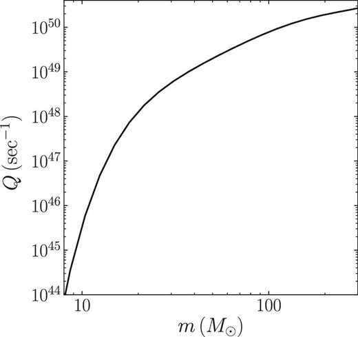
Ionizing photons per unit time as a function of stellar mass (OSTAR2002 model).
Coefficients of the polynomial fitting of |$\dot{\mathcal {N}}_{\rm LyC}$|.
| a . | b . | c . | d . | e . | f . |
|---|---|---|---|---|---|
| −39.3178 | 221.997 | −227.456 | 117.410 | −30.1511 | 3.06810 |
| a . | b . | c . | d . | e . | f . |
|---|---|---|---|---|---|
| −39.3178 | 221.997 | −227.456 | 117.410 | −30.1511 | 3.06810 |
2.3 Radiation pressure
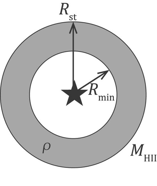
Following the analytic model of Draine (2011) and Kim, Kim, and Ostriker (2016), we also model a dusty H ii region, in which dust absorbs photons with hν > 13.3 eV, and the dust-reprocessed radiation pressure also contributes to the expansion of the H ii region. Through this effect, a central hole can be created as shown in the schematic of the H ii region in figure 2. We includes this process in the form of a velocity kick depending on the distance from the central star (r) as follows.
2.4 Other mechanical feedback
2.5 Treatment of sub-softening scale
When the molecular gas is too dense, we sometimes encounter a situation in which the Strömgren radius is too small to include at least one gas particle. If we did not add any energy to gas particles in such a case, we would underestimate the strength of the feedback. To solve this issue, we add the momentum feedback to gas particles within the gas softening length using equation (9). Instead of |$M_{\rm H\,{\small II}}$|, we adopt the total gas mass within the gas softening length, Msoft.
We also add thermal energy to the nearest gas particle by increasing the temperature of the gas particle, with an upper limit of 104 K. The temperature is determined to be proportional to the gas mass inside the Strömgren radius. We also set the minimum mass to give the momentum feedback to prevent a small gas mass from obtaining too strong a kick. The typical minimum mass is set to be the initial gas particle mass. In figure 3, we summarize the procedures of our scheme.
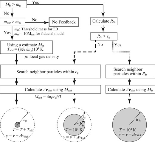
We also treat star formation as a sub-softening scale physics. When a gas particle satisfies the star formation condition (threshold density, temperature, and converging flow), a star particle is created. The mass of the forming star is chosen from a given initial mass function. In our code, however, we do not allow stars whose masses exceeds the local gas mass to form. We set a parameter, rmax, which defines a radial region where gas particles can contribute to the star formation. The mass of the forming star is limited to the half of the gas mass within rmax. This assumption naturally relates the mass of the most massive star and the total stellar mass of the host star cluster. The value of rmax depends on the resolution of the simulation and must be large enough to form massive stars (see Paper I for more details). A typical value is in the range of 0.1–0.5 pc for our targeting resolution. This corresponds to a gas-particle mass of 0.01–0.1 M⊙.
2.6 Initial conditions
Using ASURA+BRIDGE including our feedback model, we perform a series of N-body simulations of star-cluster formation starting from turbulent molecular clouds. We adopt a model similar to that of Kim, Kim, and Ostriker (2018) as initial conditions, which are homogeneous spherical molecular clouds with turbulent velocity field k = −4. In Kim, Kim, and Ostriker (2018), radiation hydrodynamics (RHD) simulations were performed with a sink method and their dusty H ii region model. Although we do not solve radiation transfer, we adopt an H ii region model based on their model (see appendix 2). We therefore compare our results with theirs. In their simulation, the model results in the formation of several small clusters, although each stellar particle represents a cluster.
We set up our model following their fiducial model (M1E5R20), with a total gas mass of Mg = 105 M⊙ and an initial radius of rg = 20 pc. We set the initial virial ratio (αvir = |Ek|/|Ep|) to be 1, where Ek and Ep are the kinetic and potential energy, respectively. Thus, this model is initially super-virial. We adopt an initial temperature of 20 K and a gas-particle mass (mg) of 0.1 M⊙.
We take the same parameters as those in model “Low” of Paper II. The gas softening is εg = 14000 au (0.07 pc), the star formation threshold density is nth = 5 × 105 cm−3, and the temperature is 20 K. The star formation efficiency is c* = 0.02. We do not use softening for stars, i.e., εs = 0.0. These parameters are summarized in table 2. Three models, K18R20noFB (without feedback from massive stars), K18R20HII (with H ii feedback), and K18R20HIIsw (with H ii feedback and velocity feedback due to stellar wind), are compared. To test the dependence on the mass resolution, we run a model (K18R20HIIm001) with a high mass resolution, mg = 0.01 M⊙, in which the other parameters are the same as those in model K18R20HII.
| Name* . | Mg . | mg . | Rg . | nini . | αvir . | tff, ini . | εs . | εg . | nth . | rmax . | Feedback . | |
|---|---|---|---|---|---|---|---|---|---|---|---|---|
| . | (M⊙) . | (M⊙) . | (pc) . | (cm−3) . | (Myr) . | . | (pc) . | (pc) . | (cm−3) . | (pc) . | H ii . | SW . |
| K18R20noFB | 1 × 10⁵ | 0.1 | 20 | 86 | 1 | 4.7 | 0.0 | 0.07 | 5 × 10⁵ | 0.2 | N | N |
| K18R20HII | 1 × 10⁵ | 0.1 | 20 | 86 | 1 | 4.7 | 0.0 | 0.07 | 5 × 10⁵ | 0.2 | Y | N |
| K18R20HIIm001 | 1 × 10⁵ | 0.01 | 20 | 86 | 1 | 4.7 | 0.0 | 0.07 | 5 × 10⁵ | 0.2 | Y | N |
| K18R20HIIsw | 1 × 10⁵ | 0.1 | 20 | 86 | 1 | 4.7 | 0.0 | 0.07 | 5 × 10⁵ | 0.2 | Y | Y |
| F20HII | 1 × 10⁵ | 0.1 | 20 | 86 | 0.25 | 4.7 | 0.0 | 0.07 | 5 × 10⁵ | 0.2 | Y | N |
| F20HIIsw | 1 × 10⁵ | 0.1 | 20 | 86 | 0.25 | 4.7 | 0.0 | 0.07 | 5 × 10⁵ | 0.2 | Y | Y |
| F20HIIswm001 | 1 × 10⁵ | 0.01 | 20 | 86 | 0.25 | 4.7 | 0.0 | 0.07 | 5 × 10⁵ | 0.2 | Y | Y |
| K18R20HII-soft | 1 × 10⁵ | 0.1 | 20 | 86 | 1 | 4.7 | 0.07 | 0.07 | 5 × 10⁵ | 0.2 | Y | N |
| K18R20HIIm001-soft | 1 × 10⁵ | 0.01 | 20 | 86 | 1 | 4.7 | 0.07 | 0.07 | 5 × 10⁵ | 0.2 | Y | N |
| K18R20HII-soft-L | 1 × 10⁵ | 0.1 | 20 | 86 | 1 | 4.7 | 0.27 | 0.27 | 3 × 10³ | 0.5 | Y | N |
| F20HIIsw-soft | 1 × 10⁵ | 0.1 | 20 | 86 | 0.25 | 4.7 | 0.07 | 0.07 | 5 × 10⁵ | 0.2 | Y | Y |
Here, “HII” indicates a H ii region model including radiation pressure model and “sw” indicates a stellar wind model; “soft” indicates “with softening” for stars, and “L” indicates low resolutions of softening for stars and gas.
| Name* . | Mg . | mg . | Rg . | nini . | αvir . | tff, ini . | εs . | εg . | nth . | rmax . | Feedback . | |
|---|---|---|---|---|---|---|---|---|---|---|---|---|
| . | (M⊙) . | (M⊙) . | (pc) . | (cm−3) . | (Myr) . | . | (pc) . | (pc) . | (cm−3) . | (pc) . | H ii . | SW . |
| K18R20noFB | 1 × 10⁵ | 0.1 | 20 | 86 | 1 | 4.7 | 0.0 | 0.07 | 5 × 10⁵ | 0.2 | N | N |
| K18R20HII | 1 × 10⁵ | 0.1 | 20 | 86 | 1 | 4.7 | 0.0 | 0.07 | 5 × 10⁵ | 0.2 | Y | N |
| K18R20HIIm001 | 1 × 10⁵ | 0.01 | 20 | 86 | 1 | 4.7 | 0.0 | 0.07 | 5 × 10⁵ | 0.2 | Y | N |
| K18R20HIIsw | 1 × 10⁵ | 0.1 | 20 | 86 | 1 | 4.7 | 0.0 | 0.07 | 5 × 10⁵ | 0.2 | Y | Y |
| F20HII | 1 × 10⁵ | 0.1 | 20 | 86 | 0.25 | 4.7 | 0.0 | 0.07 | 5 × 10⁵ | 0.2 | Y | N |
| F20HIIsw | 1 × 10⁵ | 0.1 | 20 | 86 | 0.25 | 4.7 | 0.0 | 0.07 | 5 × 10⁵ | 0.2 | Y | Y |
| F20HIIswm001 | 1 × 10⁵ | 0.01 | 20 | 86 | 0.25 | 4.7 | 0.0 | 0.07 | 5 × 10⁵ | 0.2 | Y | Y |
| K18R20HII-soft | 1 × 10⁵ | 0.1 | 20 | 86 | 1 | 4.7 | 0.07 | 0.07 | 5 × 10⁵ | 0.2 | Y | N |
| K18R20HIIm001-soft | 1 × 10⁵ | 0.01 | 20 | 86 | 1 | 4.7 | 0.07 | 0.07 | 5 × 10⁵ | 0.2 | Y | N |
| K18R20HII-soft-L | 1 × 10⁵ | 0.1 | 20 | 86 | 1 | 4.7 | 0.27 | 0.27 | 3 × 10³ | 0.5 | Y | N |
| F20HIIsw-soft | 1 × 10⁵ | 0.1 | 20 | 86 | 0.25 | 4.7 | 0.07 | 0.07 | 5 × 10⁵ | 0.2 | Y | Y |
Here, “HII” indicates a H ii region model including radiation pressure model and “sw” indicates a stellar wind model; “soft” indicates “with softening” for stars, and “L” indicates low resolutions of softening for stars and gas.
We also perform the same simulations as for models K18R20HII and K18R20HIIm001 but with softening for stars, for comparison. These models (K18R20HII-soft and K18R20HIIm001-soft in table 2) apply a softening length equal to that of gas particles.
To understand the effects of the resolution, we set up model K18R20HII-soft-L, in which a parameter set similar to model M1E5R20 in Kim, Kim, and Ostriker (2016) is used. In the model in Kim, Kim, and Ostriker (2016), a spacial resolution (grid size) of 0.3125 pc and threshold density for sink formation of 7.8 × 103 cm−3 are adopted. For comparison, we use the gas softening length εg = 70000 au (0.27 pc) and star formation density threshold nth = 3 × 103 cm−3. This set resolves the Jeans mass with 50 SPH particles. As the threshold density is lower, we set rmas = 0.5 pc. The other parameters for model K18R20HII-soft-L are the same as those of model K18R20HII-soft.
We set rmax = 0.2 pc for all models except model K18R20HII-soft-L, where rmax = 0.5 pc. The minimum mass for feedback is set to be 8 M⊙. The minimum value to give the H ii feedback is set to be 0.1 M⊙, but 0.03 M⊙ is used for models with mg = 0.01 M⊙ to avoid too large a feedback velocity due to the small included gas mass. If the Strömgren radius reaches 30 pc, we switch off the H ii feedback from the massive star. Such a large H ii region appears when a massive star escapes from the system due to strong dynamical scattering in simulations without softening. When a massive star runs to the empty region out of the cloud, the estimated Strömgren radius increases too much due to the excessively low density of gas. This is an artificial effect caused by assuming an isolated molecular cloud as an initial condition. To avoid such an artificial effect, we need to set a maximum Strömgren radius similar to the size of the entire system.
In addition, we set up four models referring to Fukushima et al. (2020). In these models, the initial virial ratio of gas is 0.25 (sub-virial) and the others are the same as those of Kim, Kim, and Ostriker (2018). As the star formation efficiency depends on the initial virial ratio of molecular clouds, this model is expected to form more stars. We note that Fukushima et al. (2020) used an AMR code with a sink method and a radiation transfer model that is different from those used in Kim, Kim, and Ostriker (2018). Model F20HIIsw-soft has softening for stars, model F20HIIsw has no softening, model F20HII has no stellar wind feedback, and model F20HIIswm001 has a high mass resolution (see table 2).
2.7 Integration
Here, we summarize the parameters used for the integration with ASURA+BRIDGE. The stars are integrated with the sixth-order Hermite scheme with individual timesteps or PeTar (see subsection 2.1 and Paper II). We adopt a timestep for the Bridge scheme of Δt = 200 yr. It is determined from the local dynamical (free-fall) time, mass resolution, and softening length of the gas (see Paper II for more details). In the presence of feedback, we also need to consider the timescale of the mechanical feedback. In our simulations, the feedback velocity is smaller than 100 km s−1 and our stepsize is short enough to resolve this motion.
We set the accuracy parameter for the Hermite individual timestep (Makino & Aarseth 1992; Nitadori & Makino 2008) to 0.2 and 0.01 for the sixth-order Hermite scheme and PeTar, respectively. As PeTar in ASURA cannot treat gravitational softening, we use the sixth-order Hermite scheme for all runs with gravitational softening for stars. For runs without softening, we first use the sixth-order Hermite scheme and switch to PeTar after the number of star particles becomes sufficiently large, as the P3T scheme is based on a tree code, and therefore the overhead of the tree code is too large for a small number of particles.
3 Star cluster formation simulations with feedback
3.1 Super-virial case
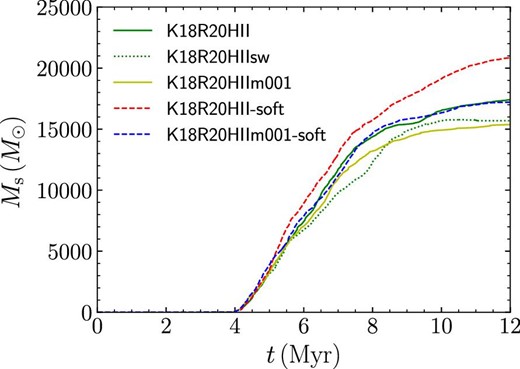
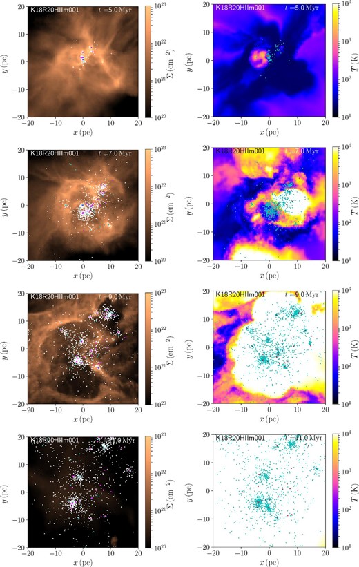
In figure 4, we present snapshots of models Kim18R20HII-soft. The time evolution of the total stellar mass formed in these simulations is shown in figure 5. The star formation starts at around the initial free-fall time (∼5 Myr). Once massive stars form, stellar feedback is switched on. In the early phase, however, the feedback energy is insufficient to stop the star formation, and therefore, the star formation in the system continues. Star formation occurs not only in the center of the entire system but in several clumps, which finally evolve into several clusters.
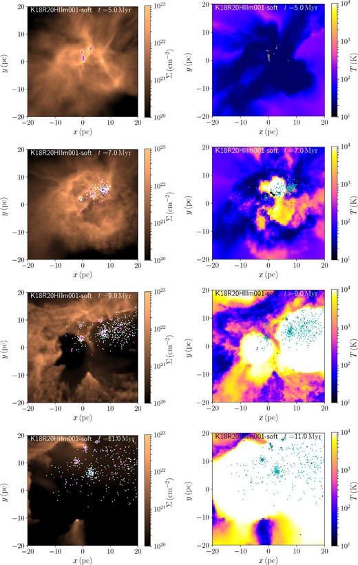
Time evolution of the distribution of gas and stars for models K18R20m001HII-soft. Left: White, blue, and magenta dots indicate stars with masses of 1–8, 8–20, and >20 |$M_{\odot}$|. The color scale indicates gas surface density. Right: Blue and red dots indicate stars with masses of 1–20 and >20 |$M_{\odot}$|, respectively. The color scale indicates the gas temperature. (Color online)
Although stellar feedback does not immediately stop the star formation, it slows it down after the formation of a few thousand stars. At ∼7 Myr (see figure 4), the H ii regions expand to the outside of the cluster. At this moment, several clumps that includes some massive stars exist in the molecular cloud. At 9 Myr, the gas inside the star-forming region is almost blown away. However, some clumps still continue star formation. Thus, the formation time of the formed clumps has a small dispersion. These individual clumps remain bound, but the separations between clumps increases (see the snapshots at 11 Myr). We will discuss the details of the formed clumps in subsection 3.4.
In figure 6, we show the snapshot of model K18R20HIIm001, in which gravitational softening for stars is not adopted. In this simulation, H ii regions form out of the central star-forming region (see snapshot at 7 Myr). These H ii regions are formed by escaping massive stars, known as runaway/walkaway stars. In figure 5, we present the time evolution of the total stellar mass of this model. The star formation is slightly suppressed in the case without softening compared to that with softening. The difference is larger in the case with lower mass resolution (models K18R20HII and K18R20HII-soft).
In figure 7, we present the mass fractions of gas and stars as a function of time for models K18R20HIIm001-soft and K18R20HIIm001. As we do not solve the chemical network, we assume that gas with T < 100 K and n > 100 cm−3 is molecular gas (Mmol), that with T > 8000 K is ionized gas (|$M_{\rm H\,{\small II}}$|), and the rest is neutral gas (Mneu). We count all gas particles that reach further than 40 pc as escaped gas (Mesc), irrespective of their densities and temperatures. Before star formation starts, more than |$60\%$| is high-density and low-temperature gas (molecular gas) and |$\sim 35\%$| is neutral gas. After 7 Myr, the amount of ionized gas starts to increase. However, the maximum is only |$\sim 10\%$|. When the feedback becomes strong enough (≳8 Myr), the fraction of escaped gas dramatically increases. The escaped gas fraction finally reaches |$\sim 70\%$| at the end of the simulation. On the other hand, the neutral and molecular gas continuously decreases. Molecular gas is converted to stars or ionized by the feedback. The fraction of ionized gas within 40 pc decreases later in the simulation. Comparing the models with and without softening, the fraction of ionized gas is slightly larger in the case without softening.
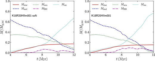
Mass fraction of gas and stars for models K18R20HIIm001-soft (left) and K18R20HIIm001 (right). Here, we define gas with T < 100 K and n > 100 cm−3 as molecular gas (Mmol), that with T > 8000 K as ionized gas (|$M_{\rm H\,{\small II}}$|), and the rest as neutral gas (Mneu). Gas particles reaching further than 40 pc are classified as escaped gas (Mesc). (Color online)
We further investigate the cause of the difference in the cases with/without softening for stars. In figure 8, we show the stellar mass functions at the end of the simulation (t = 12 Myr). The mass function is almost identical between different models, but in the massive end, we observe some differences. In our star-by-star formation scheme, we assume the IMF of Kroupa (2001) and allow stars to form up to 150 M⊙. However, the massive end of the mass functions of the formed stars is truncated. The truncation is caused by the limited amount of mass in the star-forming regions. When the gas mass within rmax is not sufficient to form a mass chosen from the given mass function, we choose a sufficiently small mass for the forming star. Such a truncation is also seen in the mass functions of observed open clusters (Weidner & Kroupa 2006). If we switch off the feedback (see model K18R20noFB-soft), the truncation mass grows to higher mass compared with the cases with feedback.
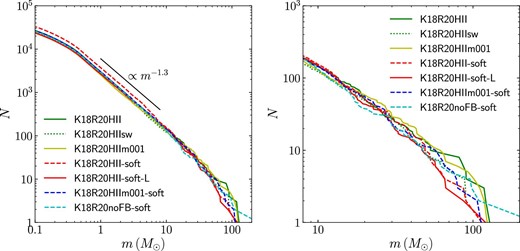
Mass functions obtained at t = 12 Myr. Left: Entire mass function. Right: Mass function of massive stars. (Color online)
This limit works in the super-virial models, in which stars form in small stellar clumps. The amount of gas in clumps cannot be sufficient to form massive stars up to the upper mass limit of the mass function, and therefore the mass of the most massive star in clumps is lower than the upper mass limit of the given mass function. With stellar softening, massive stars formed in clumps cannot be kicked out due to the interactions with binaries and so they stay inside clumps. The massive stars in clumps ionize the gas and terminate the star formation before forming more massive stars. However, without stellar softening, massive stars can be ejected from clumps, and as a consequence, star formation can continue for longer. During the more extended star formation period, clumps can accumulate more gas and form more massive stars. This difference alters the shape of the mass function at the massive end. Therefore, more ionizing photons are emitted from the massive stars in the models without softening. This is confirmed in the time evolution of Q [see figure 1 and equation (2)] shown in figure 9, where we count Q from all massive stars formed.
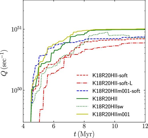
Evolution of the total photon counts from all massive stars (>8 |$M_{\odot}$|). (Color online)
To understand the relation between feedback and star formation in the cases with/without softening, we present the total mass of cold (<100 K) and dense (>106 cm−3) as a function of the total ionizing photon counts from all massive stars in figure 10. Here, we only compare models K18R20HII-soft and K18R20HII, because the star formation is not significantly different in other models with a higher mass resolution. As shown in this figure, dense cold gas forms massive stars and the ionizing photon counts increase, and then the photon counts start to decrease due to the ionization and quenching of the star formation. In the model without softening, the total amount of dense gas is initially smaller than that in the model with softening, and maintains a small value almost all the time. However, the dense gas survives longer after the formation of massive stars in the case with softening. This is because some massive stars escape from the star-forming regions as runaways due to dynamical interactions. Such runaways ionize less-dense regions in the system outside of star-forming clumps. Therefore, the star formation continues longer in the models with softening, and as a consequence more low-mass stars form.
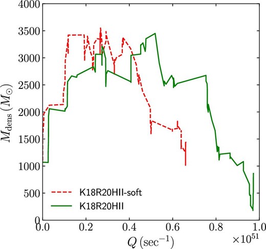
Relation between the total ionization photon counts per second from all massive stars (>8 |$M_{\odot}$|) and the total mass of dense cold gas (n > 106 cm−3 and T < 100 K). (Color online)
In figure 11, we present the evolution of the half-mass radius of the entire stellar system. The system is unbound and continues to expand after the gas expulsion, whereas individual clusters are bound (see figure 6). The details of these clusters are discussed in subsection 3.5. The entire system is more compact with stellar softening before the gas expulsion. In the model K18R20HIIsw with stellar wind feedback, the stellar wind slightly suppresses the star formation, but the effect is small.
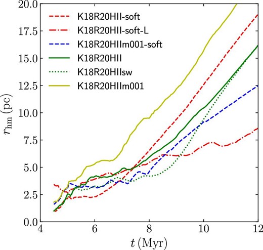
Evolution of the half-mass radius of the entire stellar system for K18R20 models. (Color online)
3.2 Sub-virial case
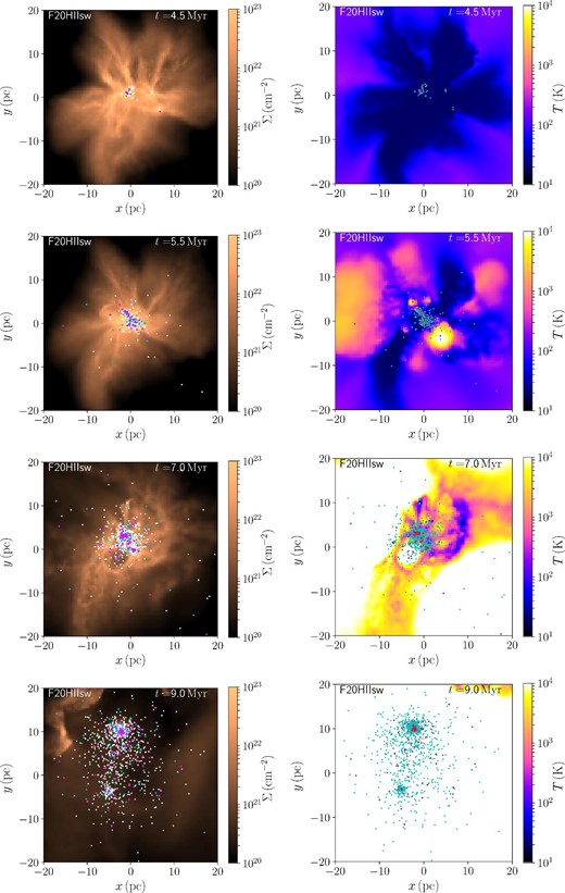
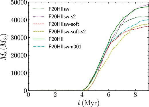
In figures 12 and 13, we present snapshots of models F20HIIsw-soft and F20HIIsw. These models are initially sub-virial. Therefore, the stellar distribution is less clumpy, and one massive cluster forms. The evolution of the total stellar mass is shown in figure 14. The star formation starts at ∼4 Myr, which is similar to the super-virial case (K18R20 models). However, the total stellar mass is smaller with softening for stars. This is opposite to the trend in the super-virial case. We further perform additional simulations with a different random seed for the initial turbulence (models F20HIIsw-s2 and F20HIIsw-soft-s2) and confirm that this trend is not a result of random seeds (see figure 14).

In figure 15, we present the time evolution of the mass fraction of gas and stars for models with and without softening for stars. The trend of the evolution in which the molecular gas decreases as stars form is similar to that of K18R20 models. The fraction of escaped gas is much smaller than the super-viral cases. The neutral gas fraction does not decrease much. Comparing the cases with/without softening for stars, the fractions of ionized and escaped gas are larger in the case without softening than in the softened case.
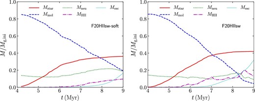
Same as figure 7 but for models F20HIIsw and F20HIIsw-soft. (Color online)
We show the stellar mass function at t = 9 Myr in figure 16 and the time evolution of the total ionizing photon counts in figure 17. Similar to the super-virial case, models without stellar softening result in the formation of a larger number of massive stars and, as a consequence, more ionizing photons compared with the models with softening. However, the difference is smaller than that in the super-virial case; with a different random seed for the initial turbulent velocity field, the formed mass functions show no clear difference between the cases with and without the stellar softening. In the sub-virial case, one massive cluster forms in the system, and therefore the given mass function can be fully sampled up to the end of the IMF.
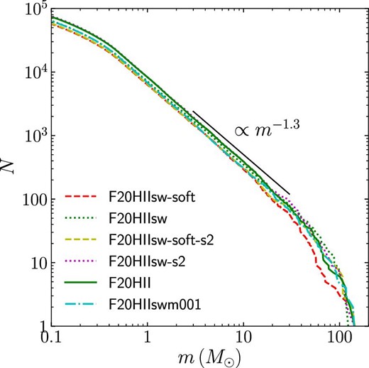
Same as the left-hand panel of figure 8 but for F20 models at t = 9 Myr. (Color online)
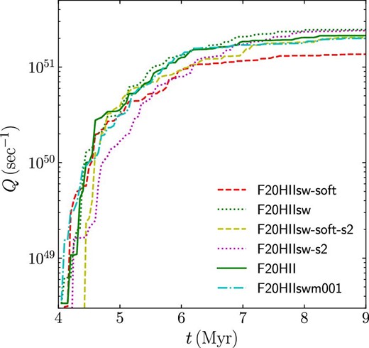
Same as figure 9 but for F20 models at t = 9 Myr. (Color online)
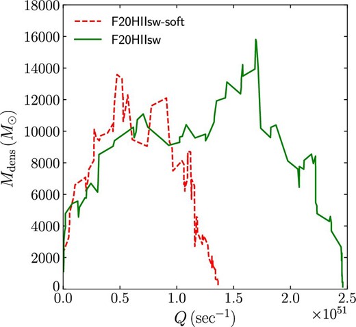
In figure 18, we present the relation between the ionizing photon counts and the amount of cold dense gas for models F20HIIsw and F20HIIsw-soft. The initial evolution is similar for both models. In both cases, the amount of cold dense gas starts to decrease after the photon counts reach ∼5 × 1051 s−1. In contrast with the super-virial case (models K18R20HII and K18R20HII-soft), the amount of dense gas increases again in the case without softening and reaches a higher peak later on. With softening, it continues to decrease after the first peak. The second peak in the case without stellar softening is due to the feedback in the outskirts of the star-forming region. As shown in figure 13, some massive stars are ejected from the central star-forming region and ionize the gas when they reach the outskirts of the cloud, in which the gas density is low enough and the H ii region can expand. The formed H ii regions push the gas toward the cloud center, and the gas in the potential well increases. This causes the second peak of the dense and cold gas mass in figure 18 and results in a higher star formation efficiency than in the model with softening.
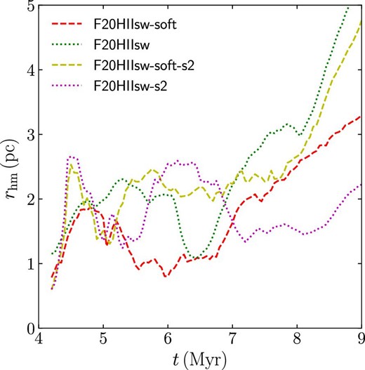
In figure 19, we present the evolution of the half-mass radius of the formed stars. Before the gas expulsion, the half-mass radius is roughly constant. The value is similar to the results in Fukushima et al. (2020) (1.5 pc). After gas expulsion, the half-mass radius starts to increase, but the central part of the formed cluster remains bound. In Fukushima et al. (2020), each stellar particle was treated as a star cluster and a cluster mass function was demonstrated. In our simulation, however, a massive cluster formed rather than a bunch of clusters.
We also present the results with a higher mass resolution (model F20HIIswm001) and without stellar-wind feedback (model F20HII) in figures 14, 16, and 17. With a higher mass resolution, the total stellar mass is slightly smaller than that with a lower mass resolution, as is also seen in the super-virial case. Without stellar-wind feedback, the total stellar mass increases, but it is within the variations due to the random seed for the initial condition.
3.3 Randomness effects
Here, we briefly discuss the effect of the randomness of these simulations. The structure of the turbulent molecular clouds and the distribution of the forming star clusters depend on the random seed for the initial turbulent velocity fields. For models F20HIIsw and F20HIIsw-soft (Seed 1), we perform another run with different random seed for the initial condition. These are models F20HIIsw-s2 and F20HIIsw-soft-s2 (Seed 2). The results are shown in figures 14, 16, 17, and 19. Compared with Seed 1, the difference in the total stellar mass between models with/without softening is smaller for Seed 2. However, the difference in the high-mass end in the mass function is not clear for Seed 2.
The formation of massive stars is another randomness in our simulations. The timing and the positions of the formation of massive stars is somehow random because we draw a mass when we form a star. The feedback process can also be affected by the randomness of the formation of runaway stars as a result of three-body encounters. The outcome of three-body encounters is highly chaotic, and therefore the mass and velocity of stars scattered from the center to the outskirts of clusters can also randomly change in each run.
3.4 Comparison with previous works
As described in subsection 2.6, we adopt models similar to those of Kim, Kim, and Ostriker (2018) and Fukushima et al. (2020). Hereafter, we compare our results with these studies, in which they performed simulations using grid-based codes, sink methods, and super-particles for stars with softening.
Figure 20 shows the stellar mass evolution of our models. Compared to those in Kim, Kim, and Ostriker (2018), the star formation proceeds for longer in our simulations, and the final stellar mass is larger (see models K18HII-soft and K18HIIm001-soft). This may be due to the difference in softening lengths adopted in our simulation and in theirs. We additionally perform a simulation with a larger softening length, which is similar to the grid size adopted in Kim, Kim, and Ostriker (2018), named as model K18R20HII-soft-L. The final stellar mass at 12 Myr (∼1.2 × 10⁴ M⊙) is smaller than for model K18R20HII-soft, and it is similar to that obtained in Kim, Kim, and Ostriker (2018).
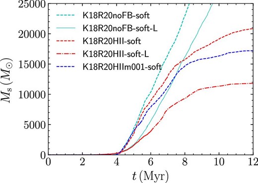
Kim, Kim, and Ostriker (2018) also performed their simulations with higher and lower resolutions, and confirmed that the final stellar mass evolution converges. In our simulation, in contrast, the star formation proceeds slightly more rapidly with a run with smaller softening for gas (similar to higher spatial resolution). This results in the formation of more stars in our simulation (model K18R20HII). We can confirm that star formation is more efficient for a smaller softening in models without feedback (models K18R20noFB-soft and K18R20noFB-soft-L; see figure 20). Thus, the rapid increase in forming stars with a smaller softening length causes the slightly higher star-formation efficiency in our simulation.
We also compare our results (F20 models) with that of Fukushima et al. (2020). Our models, even including the stellar wind, form roughly twice as many stars as theirs (∼2 × 10⁴ M⊙). The difference comes from the difference in the treatment of stellar particles and the related mass function. As shown in figure 16, the high-mass end of the mass function of the formed stars is truncated in our simulations. In Fukushima et al. (2020), in contrast, the mass function is assumed to continue up to 150 M⊙ following the Chabrier mass function (Chabrier 2003). In their model, they used the photon production rate per unit mass, s* = 8.0 × 1046 s|$^{-1}\, {M}_{{\odot} }^{-1}$|. As the final stellar mass in their simulation was ∼2 × 10⁴ M⊙, the ionizing photon count was estimated to be 1.8 × 1051 per second. This is ultimately comparable to ours (see figure 17). Thus, the number of photons necessary to ionize the entire system is similar in both simulations, but the total stellar masses required to reach that point are different.
Thus, we confirm that our feedback models give results similar to previous simulations performed using radiation hydrodynamics codes. We also find positive and negative effects of the stellar feedback on the star formation when we correctly treat the dynamical evolution of star clusters. We identify a small dependence of the total stellar mass on the gas-particle mass, although we might underestimate the feedback for the H ii region model. When the gas density is high, there are only a few gas particles within the Strömgren radius. If the gas mass within the Strömgren radius estimated from the gas density is for 2.5 gas particles, we consider the feedback energy for only two particles and ignore the feedback energy for 0.5 particles. This treatment underestimates the feedback energy, especially if the mass resolution of gas is low.
3.5 Formation and evolution of star clusters
We further compare the star clusters formed in our simulations with observations and previous theoretical works. We detect clusters from the snapshots for models K18R20HII and K18R20HIIm001 at 5, 6, 7, 9, and 11 Myr using HOP (Eisenstein & Hut 1998) in AMUSE. HOP is an algorithm that detects clumps using local stellar densities. We use the same parameter set as that used in Fujii (2019). After 8 Myr, most clumps are almost gas-free. We therefore select dynamically bound particles and count them as cluster members at 9 and 11 Myr. In contrast, clumps are embedded in the gas at an earlier time. We count all particles chosen by HOP as cluster members (<8 Myr). The minimum number of stars for the detection is 100. As the expected mean stellar mass is ∼0.5 M⊙, clusters of ≲50 M⊙ are ignored in our analysis. We then calculate the half-mass radius (rh, cl) and half-mass density (ρh, cl) of the detected clusters. There is no clear difference in the mass and radius distributions of the two models, although the mass resolution for gas is different.
In figure 21, we present the spatial distribution of the detected clusters at 9 and 11 Myr for model K18R20HIIm001. We indicate the half-mass radii and masses by the sizes of the circles and crosses. We confirm that our clump-finding method can detect major clumps (see also figure 6). Note that some clumps are found to have a much higher mean mass that than expected from the given mass function (∼0.5 M⊙). This may be due to the clump-finding methods. In the following figures, we present clumps with a mean stellar mass larger than 0.8 M⊙ with small symbols.
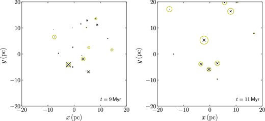
Cluster distribution of model K18R20HIIm001 at t = 9 (left) and 11 (right) Myr. Yellow circles represent the half-mass radii. Black crosses indicate the center-of-mass positions. The sizes of crosses represent the cluster masses. (Color online)
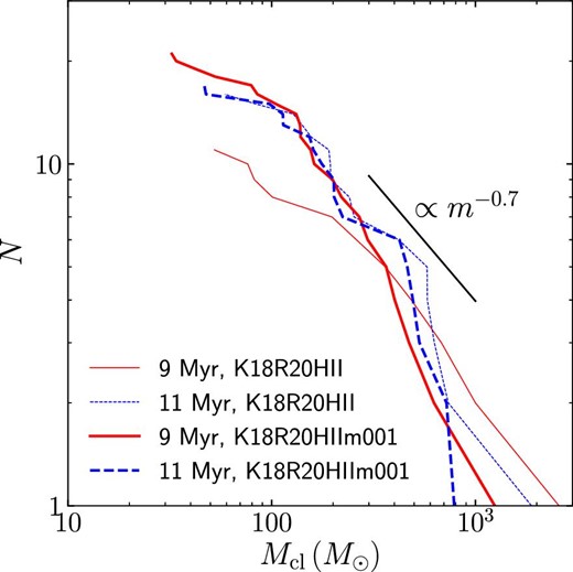
Cumulative cluster mass function of K18R20 models. (Color online)
Fujii and Portegies Zwart (2015) obtained a value for the power of their obtained cluster mass function as α = −1.7. In figure 22, we also present this relation. As our number of obtained clusters is only ∼ 20 per simulation, it is difficult to fit a power law to our cluster mass function, but the power is apparently shallower than −2.
We also show the relation between cluster mass and half-mass radius in figure 23. At ≲ 7 Myr, the clusters are still embedded in the gas (see figure 6). Therefore, we did not check if the selected stars bound to the cluster or not. At this earlier time, the obtained clusters have radii much smaller than those typical of currently observed open clusters (see figure 2 of Portegies Zwart et al. 2010). After gas expulsion due to the stellar feedback (t ≳ 9 Myr), the half-mass radius expands. The radius after gas expulsion is consistent with the densest open clusters shown in figure 2 of Portegies Zwart, McMillan, and Gieles (2010). For t = 9 and 11 Myr, the masses of bound stars are shown.
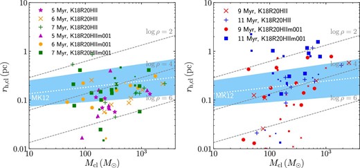
Relation between the mass and half-mass radius of embedded clusters (left) and bound clusters (right) detected in models K18R20HII and K18R20HIIm001. The light blue shaded region and white dotted line indicate equation (11). Small symbols indicate clusters with mean stellar mass of >0.8 |$M_{\odot}$|. (Color online)
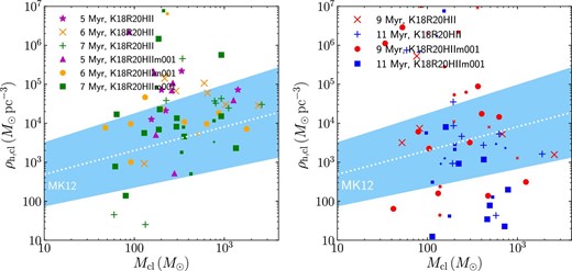
Relation between the mass and half-mass density of embedded clusters (left) and bound clusters (right) detected in models K18R20HII and K18R20HIIm001. The light blue shaded region and white dotted line indicate equation (12). Small symbols indicate clusters with mean stellar mass of >0.8 |$M_{\odot}$|. (Color online)
We also compare our results with a similar simulation, but assuming instantaneous star formation and gas expulsion performed by Fujii and Portegies Zwart (2016). The mass and radius obtained in both simulations are similar (100 < Mcl < 103 M⊙ and 0.1 < rhm, cl < 1 pc). Thus, the simplified star formation and gas expulsion models adopted by Fujii and Portegies Zwart (2016) are sufficient to study cluster mass function and dynamical evolution of clusters after gas expulsion.
We further investigate the stellar ages in our formed clusters. In figure 25, we present the age distribution of stars in the six most massive clusters detected at t = 11 Myr for model K18R20HIIm001. The age distribution varies for each cluster. One of the biggest clusters continues star formation for ∼5 Myr, while another forms most of its stars within ∼1 Myr. There are also ones with double and triple peaks in the age distribution. These are a result of hierarchical formation (Fujii et al. 2012; Fujii 2015). Multiple peaks of stellar ages in one cluster have also been observed in the Orion Nebula Cluster (Beccari et al. 2017).
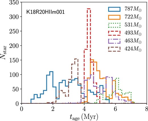
Stellar age distribution of the six most massive clusters at t = 11 Myr in model K18R20HIIm001. (Color online)
We also show the relation between cluster mass and age with the dispersion (standard deviation) in figure 26. We find a trend that more massive clusters form earlier, although the scatter is large. This is probably related to our initial condition, which is an initially homogeneous sphere. The gas cloud first gravitationally collapses before star formation starts in the center of the cloud, which is the densest region. Hence, the most massive clusters form around the cloud center (see figure 6). In contrast, small clumps can form in the outskirts of the cloud, even after the feedback starts to eject the gas from the most massive clusters.
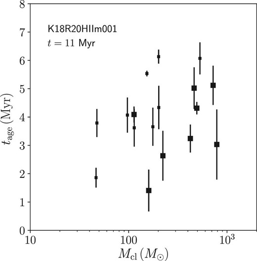
Age (mean stellar age) and age spread among cluster members for clusters detected at t = 11 Myr as a function of cluster mass for model K18R20HIIm001. Small symbols indicate clusters with mean stellar mass of >0.8 |$M_{\odot}$|.
We also detect the clusters formed in the model F20HIIsw. As shown in figure 13, one massive cluster was formed in our sub-virial models. The bound mass of the most massive cluster at t = 9 Myr is 12000 M⊙, which is comparable to the masses of young massive clusters such as NGC 3603 and Trumpler 14 (Portegies Zwart et al. 2010). In figure 27, we present the surface density profile of this cluster. The core radius calculated using the method of Casertano and Hut (1985) is 0.33 pc, which is larger than that of NGC 3603 (0.15 pc) and Trumpler 14(0.14 pc). The half-mass radius of the cluster in our simulation is 0.61 pc, while the effective radii of NGC 3603 and Trumpler 14 are 0.7 and 0.5 pc, respectively (Portegies Zwart et al. 2010). In figure 28, we show the age distribution of the cluster at t = 9 Myr. There is a peak at ∼2.5 Myr, a few small sub-peaks, and an elongated distribution.
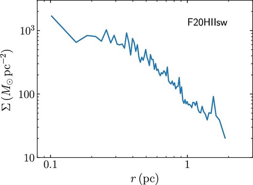
Surface density profile of the most massive cluster at t = 9 Myr in model F20HIIsw. (Color online)
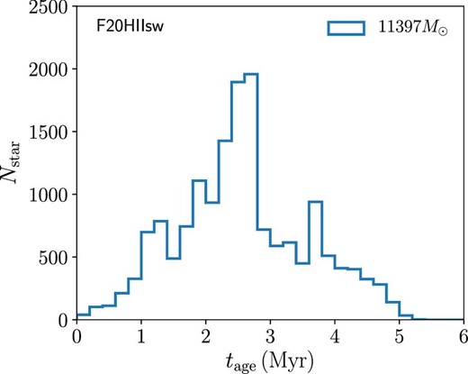
Stellar age distribution of the most massive cluster at t = 9 Myr in model F20HIIsw. (Color online)
Banerjee and Kroupa (2015) studied the hierarchical formation of young massive clusters using N-body simulations without softening, although the gas potential is static in their simulations. Their results suggest that either a monolithic or a hierarchical formation within 1 Myr is preferable for NGC 3603, which is a young massive cluster in the Milky Way. Our result also supports the formation of young massive clusters in a short period.
We also investigate the fraction of mass remaining in bound clusters at the end of the simulations. For the model K18R20HIIm001 (the super-virial case), 5500 M⊙ stars belong to bound clusters. This mass is |$37\%$| of the total stellar mass formed in the simulation. For the model F20HIIsw (sub-virial case), 15000 M⊙ stars belong to bound clusters. This mass is |$36\%$| of the total stellar mass. Thus, about one-third of stars belong to bound clusters after the gas expulsion in our simulations.
4 Summary
We developed a new tree-direct hybrid code, ASURA+BRIDGE (Paper II), in which stars are realized as individual stars following a realistic mass function and are integrated using high-order integrators and sixth-order Hermite (Nitadori et al. 2006) and P3T schemes (Wang et al. 2020a). In this code, we implemented stellar feedback schemes: thermal feedback due to radiation from massive stars and mechanical feedback due to the radiation and stellar wind. For the radiation, we adopted a model giving thermal feedback within a Strömgren radius calculated from the gas density and radiation of massive stars. The ionization photon counts were estimated using OSTAR2002 (Lanz & Hubeny 2003). We also implemented the dusty feedback model of Kim, Kim, and Ostriker (2016).
Using this new code, we performed simulations of star cluster formation from turbulent molecular clouds. In these simulations, we adopted a probabilistic star formation scenario, in which star formation happens statistically. The star formation rate depends on the local density. The stellar mass was drawn from a given stellar mass function (Paper I). In this scheme, we were able to achieve a star-by-star treatment without using an extremely high resolution for the gas particle mass. Moreover, the integration of stellar orbits did not require softening. Thus, we were able to properly investigate the dynamical evolution of star clusters.
To compare our results with previous works, we performed simulations of models similar to those of Kim, Kim, and Ostriker (2018) and Fukushima et al. (2020) with/without gravitational softening. Without softening, some stars experienced close encounters with other stars in dense star-forming regions. These close encounters kicked stars out of clusters. In particular, once tight binaries formed, even massive stars that had formed inside clusters were ejected. We found that such runaway massive stars escaped from the cluster center (dense region) to ionize the gas in the outskirts of the star-forming regions. With softening, in contrast, massive stars were kept inside clusters and ionization proceeded inside the forming clusters.
The difference with/without softening in the stellar mass evolution is not simple. When the system is super-virial, star formation is suppressed with softening for stars. In this case, ejected massive stars ionize the gas from the outskirts of the star-forming regions. This stops star formation at a later time. In sub-virial cases, in contrast, star formation is enhanced without softening for stars. In this case, one massive cluster forms in the cloud center, and it also ejects some massive stars, which ionize the gas as they reach outer, less dense regions. With this feedback, some gas is compressed. As a result, the star-formation rate increases. Our results are consistent with those of previous studies using radiation hydrodynamics simulations, in which the radiation was correctly treated but stars were treated as super-particles. With a softening length similar to that in Kounkel et al. (2018), we obtained a similar final stellar mass in the initially super-virial cloud model. In the case of sub-virial models, which were compared to those in Fukushima et al. (2020), we obtained a higher star-formation efficiency. This may be due to the lack of high-mass stars in our simulations, which is also seen in observations of star clusters in the Milky Way.
We further investigated the mass and radius relation of clusters formed in our simulations and compared them with observations and theoretical studies. Our results suggest that star clusters initially had densities much higher than those of currently observed open clusters. This result supports the analytical estimate reported in Marks and Kroupa (2012). Our results suggest that the densities of open clusters were 103–105 M⊙ pc−3 when they were embedded in their parental gas. However, the variation in the density is quite large.
The star-formation history also has a large variation. The most massive cluster in our super-virial model contained stars with an age distribution over 5 Myr. The distribution of this cluster showed three peaks caused by the hierarchical formation of star clusters. In contrast, another cluster showed a formation period of only ∼1 Myr. With our sub-virial initial condition, one massive cluster was formed, and its mass and radius were comparable to those of young massive clusters in the Milky-Way galaxy. In both super- and sub-virial cases, about one-third of stars remain in the bound clusters after gas expulsion. We will further investigate the star-cluster formation process using models with different initial conditions for gas in a forthcoming paper.
Our model currently does not consider the mass loss from massive stars due to stellar wind, the supernova explosions, or the formation of compact objects like black holes. These may affect the evolution of star clusters, especially in the cluster core. Supernova explosions may terminate the relatively slow star formation with a timescale longer than the present models. We will investigate these effects in future work.
Acknowledgements
The authors thank Takashi Hosokawa for useful comments on the development of the code, Hajime Fukushima for fruitful discussion, and Steven Rieder for helping with AMUSE scripts. The authors also thank the anonymous referee for their comments to improve the manuscript. L.W. is grateful for the financial support from the JSPS International Research Fellowship (Graduate School of Science, The University of Tokyo). Numerical computations were carried out on Cray XC50 CPU-cluster at the Center for Computational Astrophysics (CfCA) of the National Astronomical Observatory of Japan and Oakbridge-CX system at the Information Technology Center, The University of Tokyo. This work was supported by JSPS KAKENHI Grant Number 19H01933, 20K14532, 21J00153, 21H04499, 21K03614, 21K03633 and MEXT as “Program for Promoting Researches on the Supercomputer Fugaku” (Toward a unified view of the universe: from large scale structures to planets, Revealing the formation history of the universe with large-scale simulations and astronomical big data), The University of Tokyo Excellent Young Researcher Program, the Initiative on Promotion of Supercomputing for Young or Women Researchers, Information Technology Center, The University of Tokyo, and the RIKEN Special Postdoctoral Researchers Program. We would like to thank Editage (www.editage.com) for English language editing.
Appendix 1. STARBENCH test
To test our model for H ii region, we perform a series of simulations similar to STARBENCH runs (Bisbas et al. 2015). STARBENCH is a project to compare numerical simulations of expanding H ii region using different codes including both 1D and 3D grid-based codes and SPH codes.
We take an initial condition similar to that used in STARBENCH (Bisbas et al. 2015) for SPH codes. Here, we describe our model, and the slight difference between its initial condition and that of STARBENCH. We assume a homogeneous sphere with a density of 5.21 × 10⁻²¹ g cm−3 with a radius of 5.82 pc, which is twice as large as that adopted in STARBENCH. The resulting total gas mass is 6.4 × 10⁴M⊙. We adopt a mass resolution of gas of mg = 0.1 M⊙ and 0.01 M⊙, which are the same as those we adopt for our cluster-formation simulations. The initial temperature of gas is set to 100 K (model SB100K). We also perform a run with cooling (model SBCo). For models with cooling, we set the initial gas temperature to be 20 K. We adopt a gravitational softening length of 10000 au for the runs with a gas particle mass of 0.1 M⊙. For the runs with 0.01 M⊙, we set the softening length to 5000 au. These models are summarized in table 3.
| Name . | mg(M⊙) . | εg (au) . | Cooling . | Other feedback . |
|---|---|---|---|---|
| SB100K | 0.1 | 10000 | N | — |
| SBCo | 0.1 | 10000 | Y | — |
| SBCoRP | 0.1 | 10000 | Y | RP |
| SBCoRPSW | 0.1 | 10000 | Y | RP, SW |
| SB100K-H | 0.01 | 5000 | N | — |
| SBCoRPSW-H | 0.01 | 5000 | Y | RP, SW |
Instead of putting a source of Q0 = 1049 photons per second, we adopt a star which emits photons with the same rate (40 M⊙ in our model). In addition, our simulations include self-gravity, and therefore the gas cloud collapses in its initial free-fall time.
![Evolution of Strömgren radius for our models and Spitzer solution [equation (A1)]. (Color online)](https://oup.silverchair-cdn.com/oup/backfile/Content_public/Journal/pasj/73/4/10.1093_pasj_psab061/2/m_psab061fig29.jpeg?Expires=1749385385&Signature=YAz-HULu63RMIG2HasxH249EY1Q~gmjthn3nLJT8GHgXcqxdozWkuMkRzySmQH8jRns57WS0~1EAzOX8OO~rTr9KtQJv2H92cMPVpwv27VggSjqKd6JT81vRrqg~mfLFLPNxTdFoe0HdFyION9zsUpeepTjjdmvOPtaBMLob3FBOQL21tewDsh7s7~to5v1BIdbl4enelCISCvbmuhW-TQxZVDjMUTSmTUt9li4wF1ameTTZmtulUlQJX-ETEzoq9JYbSPBZeSy6mB41rpPmnpm7AwW27WjZDHAvOkBVzGSmPixcU3PkBSrdnx5xFxsTjRo9GcmqnOad5uFCv5AAYg__&Key-Pair-Id=APKAIE5G5CRDK6RD3PGA)
Evolution of Strömgren radius for our models and Spitzer solution [equation (A1)]. (Color online)
We also test the case with cooling (model SBco), since our final goal is simulations with cooling. In addition, we test models with mechanical feedback due to radiation pressure [equation (8)] (model SBcoRP) and also stellar wind [equation (9)] (models SBCoRPSW). These results are also shown in figure 29. With cooling, the H ii region becomes smaller compared with the case without cooling. The radiation pressure and stellar wind slightly pushes the Strömgren radius outwards. We finally perform a run including everything with high resolution (model SBCoRPSW-H). Similar to the case without cooling, the Strömgren radius is |$\sim\!\! 10\%$| larger than the case with a lower resolution.
Appendix 2. Single-source test
To compare our dusty H ii region model with previous work performed in Kim, Kim, and Ostriker (2016), we perform a series of simulations similar to those in Kim, Kim, and Ostriker (2016). They followed the description of the radiation pressure in a dusty H ii region in Draine (2011) and used Athena to perform the RHD simulations of an expanding dusty H ii region. Their result agrees with the analytic solution from Draine (2011).
We adopt molecular clouds with uniform densities (n) of 103, 104, and 105 cm−3. For all models, the mass resolution (mg) is 0.1 M⊙. The softening length (εg) is set to be 104 au.
The initial gas temperature (Tini) is 20 and 100 K for models with and without cooling, respectively. We put a star with a mass of 60 M⊙ in the center of the gas distribution. The emission rates of ionization photons (|$Q_0=\dot{\mathcal {N}}_{\rm LyC}$|) are set to be 1049 and 1052 s−1 for models with n = 103 and 104 cm−3, respectively. We adopt a sufficiently large cloud size to retain most of the gas bound after the formation of H ii regions. This size depends on both the gas density and the emission rate. The masses and radii of gas distribution for our initial conditions are summarized in table 4. In all simulations, the feedback due to stellar wind is not included, but the self-gravity is included.
| Name . | mg (M⊙) . | εg (au) . | n (cm−3) . | Tini (K) . | Mg (M⊙) . | Rg (pc) . | Q0 (s−1) . | Cooling . |
|---|---|---|---|---|---|---|---|---|
| DHQ49n1e3 | 0.1 | 104 | 103 | 100 | 4 × 10⁵ | 14.0 | 1049 | N |
| DHQ49n1e3C | 0.1 | 104 | 103 | 20 | 4 × 10⁵ | 14.0 | 1049 | Y |
| DHQ49n1e4 | 0.1 | 104 | 104 | 100 | 2 × 10⁵ | 5.16 | 1049 | N |
| DHQ49n1e4C | 0.1 | 104 | 104 | 20 | 2 × 10⁵ | 5.16 | 1049 | Y |
| DHQ49n1e5 | 0.1 | 104 | 105 | 100 | 5 × 10⁵ | 3.25 | 1049 | N |
| DHQ49n1e5C | 0.1 | 104 | 105 | 20 | 5 × 10⁵ | 3.25 | 1049 | Y |
| DHQ50n1e4 | 0.1 | 104 | 104 | 100 | 2 × 10⁵ | 5.16 | 1050 | N |
| DHQ50n1e4H | 0.01 | 5 × 10³ | 104 | 100 | 2 × 10⁵ | 5.16 | 1050 | N |
| DHQ50n1e4C | 0.1 | 104 | 104 | 20 | 2 × 10⁵ | 5.16 | 1050 | Y |
| DHQ50n1e5 | 0.1 | 104 | 105 | 100 | 5 × 10⁵ | 3.25 | 1050 | N |
| DHQ50n1e5C | 0.1 | 104 | 105 | 20 | 5 × 10⁵ | 3.25 | 1050 | Y |
| DHQ52n1e4 | 0.1 | 104 | 104 | 100 | 2 × 10⁶ | 11.1 | 1052 | N |
| DHQ52n1e4C | 0.1 | 104 | 104 | 20 | 2 × 10⁶ | 11.1 | 1052 | Y |
From left to right: Model name, gas particle mass (mg), softening length for gas (εg), initial gas density (n), initial gas temperature (Tini), total gas mass (Mg), initial gas radius (Rg), ionizing photon emission rate Q0, and cooling model. Model names include the value of Q0, gas density (n), and the cooling.
| Name . | mg (M⊙) . | εg (au) . | n (cm−3) . | Tini (K) . | Mg (M⊙) . | Rg (pc) . | Q0 (s−1) . | Cooling . |
|---|---|---|---|---|---|---|---|---|
| DHQ49n1e3 | 0.1 | 104 | 103 | 100 | 4 × 10⁵ | 14.0 | 1049 | N |
| DHQ49n1e3C | 0.1 | 104 | 103 | 20 | 4 × 10⁵ | 14.0 | 1049 | Y |
| DHQ49n1e4 | 0.1 | 104 | 104 | 100 | 2 × 10⁵ | 5.16 | 1049 | N |
| DHQ49n1e4C | 0.1 | 104 | 104 | 20 | 2 × 10⁵ | 5.16 | 1049 | Y |
| DHQ49n1e5 | 0.1 | 104 | 105 | 100 | 5 × 10⁵ | 3.25 | 1049 | N |
| DHQ49n1e5C | 0.1 | 104 | 105 | 20 | 5 × 10⁵ | 3.25 | 1049 | Y |
| DHQ50n1e4 | 0.1 | 104 | 104 | 100 | 2 × 10⁵ | 5.16 | 1050 | N |
| DHQ50n1e4H | 0.01 | 5 × 10³ | 104 | 100 | 2 × 10⁵ | 5.16 | 1050 | N |
| DHQ50n1e4C | 0.1 | 104 | 104 | 20 | 2 × 10⁵ | 5.16 | 1050 | Y |
| DHQ50n1e5 | 0.1 | 104 | 105 | 100 | 5 × 10⁵ | 3.25 | 1050 | N |
| DHQ50n1e5C | 0.1 | 104 | 105 | 20 | 5 × 10⁵ | 3.25 | 1050 | Y |
| DHQ52n1e4 | 0.1 | 104 | 104 | 100 | 2 × 10⁶ | 11.1 | 1052 | N |
| DHQ52n1e4C | 0.1 | 104 | 104 | 20 | 2 × 10⁶ | 11.1 | 1052 | Y |
From left to right: Model name, gas particle mass (mg), softening length for gas (εg), initial gas density (n), initial gas temperature (Tini), total gas mass (Mg), initial gas radius (Rg), ionizing photon emission rate Q0, and cooling model. Model names include the value of Q0, gas density (n), and the cooling.
In order to test the effect of resolution, we perform a simulation with a higher resolution, named as DHQ50n1e4H. For this model, Q0 = 1052 s−1, n = 104 cm−1, mg = 0.01 M⊙, and εg = 5000 au. For this run, cooling is not included.
In figure 30, we present the time evolution of the Strömgren radius and its expansion velocity for all models. Since we include self-gravity, the expansion turns into
contraction at a certain time. Once that happens, we stop the simulations. The maximum radius and the time taken to reach it increase as the gas density decreases. As the ionizing photon emission rate increases, the maximum radius also increases, but the time to reach it does not.
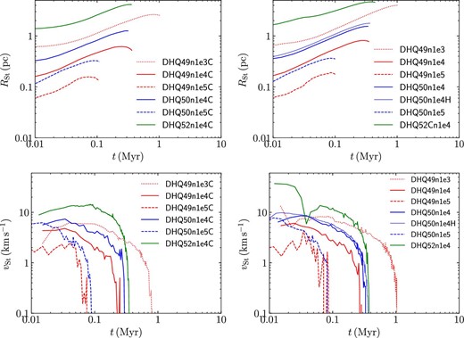
Evolution of the Strömgren radius and the expansion velocity of the shell for all models. Left- and right-hand panels are results with and without cooling, respectively. (Color online)
With cooling, the maximum radius becomes slightly smaller compared with those without cooling. This difference becomes smaller as the Strömgren radius becomes smaller. We also confirm that the resolution effect is sufficiently small by comparing models DHQ501e4 and DEQ501e4H.
We compare our results with those in Kim, Kim, and Ostriker (2016). Their figure 4 shows the results of the models similar to DHQ50n1e4 and DHQ50n1e4C. In our simulations, the H ii region in the model DHQ50n1e4 expands up to ∼1.5 pc at ∼0.3 Myr, while that in Kim, Kim, and Ostriker (2016) expands to ∼2 pc at ∼0.8 Myr. Thus, our H ii region feedback model slightly underestimates the shell expansion. On the other hand, in a stronger emission case, i.e., models DHQ52n1e4 and DHQ52n1e4C, the H ii region in our models expands more than that of Kim, Kim, and Ostriker (2016) (∼3 pc). We note that such a large emission rate cannot be reached with ionizing photon emission from only one massive star (see figure 1).
In figure 31, we present the time evolution of the radial density distributions of gas in our simulations. The models in the top (the model DHQ491e3C) and the bottom right-hand (the model DHQ521e4C) panels correspond to the models A and C in Kim, Kim, and Ostriker (2016). As is discussed in Kim, Kim, and Ostriker (2016), the radiation pressure is expected to dominate the thermal pressure when nQ49 > 104 cm−3, where Q49 = Q0/(1049 s−1). In such a regime, a hole around the source is expected to form due to the radiation pressure. Indeed, our simulations also reproduce the hole with the same criterion (see the bottom left- and right-hand panels of figure 31). The shell in our simulation is thicker than that of Kim, Kim, and Ostriker (2016), but the density is roughly consistent. In Kim, Kim, and Ostriker (2018), the shell density in Kim, Kim, and Ostriker (2016) decreases with time, because their simulations do not include self-gravity. In our simulations, on the other hand, the shell density increases with time since the cloud collapses due to the self-gravity. Thus, we confirm that our models sufficiently agree with those of Kim, Kim, and Ostriker (2018).

Evolution of the radial density distributions of expanding H ii regions. Top: model DHQ49n1e3C; bottom: DHQ50n1e4C (left) and DHQ52n1e4C (right). (Color online)
References
Author notes
JSPS Research Fellow


