


Abstract
The Antennae Galaxies, one of major mergers, are a starburst. Tsuge et al. (2020, PASJ, 73, S35) showed that the five giant molecular complexes in the Antennae Galaxies have signatures of cloud–cloud collisions based on the Atacama Large Millimeter Array (ALMA) archival data with 60 pc resolution. In the present work we analyzed the new CO data toward the super star cluster (SSC) B1 with 14 pc resolution obtained with ALMA, and confirm that two clouds show a complementary distribution with a displacement of ∼70 pc as well as connecting bridge features between them. The complementary distribution shows a good correspondence with the theoretical collision model (Takahira et al. 2014, ApJ, 792, 63), and the distribution indicates that the formation of SSC B1 with ∼106 M⊙ was consistent with the trigger of cloud–cloud collision on a time scale of ∼1 Myr, which is consistent with the cluster age. It is likely that SSC B1 was formed from molecular gas of ∼107 M⊙ with a star formation efficiency of |$\sim\! 10\%$| in 1 Myr. We identify a few places where additional clusters are forming. Detailed gas motion indicates that the stellar feedback in the accelerating gas is not effective, while the ionization plays a role in evacuating the gas around the clusters at a ∼20 pc radius. The results have revealed the details of the parent gas where a cluster having a mass similar to a globular is being formed.
1 Introduction
Super star clusters (SSCs) are attracting a keen interest of researchers, since SSCs are highly energetic and affect the galactic evolution substantially. SSCs are also supposed to be a present-day analog to the ancient globulars, the formation of which is deeply connected to the environment of the early universe. The Antennae Galaxies are an outstanding major merger where thousands of young SSCs are discovered.
Genzel, Lutz, and Tacconi (1998) showed that the galaxy mergers have excess infrared luminosity compared with the isolated galaxies, lending support for the active star formation triggered by galaxy interactions in mergers. The Antennae Galaxies are the most outstanding major merger and the closest to the Milky Way at a distance of 22 Mpc (Schweizer et al. 2008). The galaxies consist of the two spirals NGC 4038 (RA = |${12^{\rm h}01^{\rm m}53{_{.}^{\rm s}}00}$|, Dec = |$-18^{\circ }{52^{\prime }10^{\prime \prime }}$|) and NGC 4039 (RA = |${12^{\rm h}01^{\rm m}53{_{.}^{\rm s}}60}$|, Dec = |$-18^{\circ }{53^{\prime }11^{\prime \prime }}$|). The interaction between NGC 4038 and NGC 4039 has been continuing probably since a few 100 Myr ago (Mihos et al. 1993; Karl et al. 2010; Renaud et al. 2015 and references therein). The Antennae Galaxies are prominent because of the unusually active star formation (often called “starbursts”) including thousands of young massive SSCs (e.g., Whitmore & Schweizer 1995), and clear signatures of the galactic interaction in the forms of two long tails.
At a smaller distance, we have increasing evidence for similar cloud–cloud interactions triggering the formation of SSCs, which include R136 in the Large Magellanic Cloud (LMC; Fukui et al. 2017) and NGC 604 in M 33 (Tachihara et al. 2018) as well as several SSCs in the Milky Way (Furukawa et al. 2009; Ohama et al. 2010; Fukui et al. 2014, 2016; Kuwahara et al. 2021; Fujita et al. 2021). Also see a review paper of the cloud-cloud collision (Fukui et al. 2021) for the latest results of observational and theoretical studies.
Molecular observations are crucial in studying cluster formation in mergers. In particular, the Atacama Large Millimeter Array (ALMA) offers an ideal opportunity to investigate the molecular gas distribution and kinematics with the highest resolution achieved so far, which are possibly related not only to the feedback by the SSCs but also directly to the SSC formation.
The previous works on the ALMA data investigated the distribution of molecular clouds and dense gas (Whitmore et al. 2014; Schirm et al. 2016), the effect and mechanism of stellar feedback (Herrera & Boulanger 2017), and progenitors of SSCs (Herrera et al. 2011, 2012; Johnson et al. 2015), whereas the mechanism of cluster formation has not been well understood. Whitmore et al. (2014) briefly suggested a possible role of filamentary cloud collision induced by tidal interaction in SSC formation, but no further exploration of cluster formation was undertaken in these articles. Most recently, Tsuge et al. (2020) (hereafter Paper I) studied the ALMA CO data and presented evidence for cloud–cloud collisions in the five giant molecular cloud complexes, opening a new window on the pursuit of SSC formation. These authors used ALMA Cycle 0 data with 50 pc resolution, while the Firecracker, an SSC candidate, was studied with 10 pc resolution of Cycle 4 (Finn et al. 2019) and a complementary distribution between two colliding clouds was revealed.
In the Antennae, 40% of the youngest SSCs are located in the overlap region, as indicated in figure 1a, where two galaxies are merging (Wilson et al. 2000). The SSCs are cataloged by using the near-infrared data taken with the Hubble Space Telescope (Gilbert & Graham 2007; Whitmore et al. 2010). About 60% of the 50 most massive clusters, which have masses greater than ∼6 × 10⁵ M⊙, are located in the overlap region (Whitmore et al. 2010). Five out of eight SSCs with masses larger than 106 M⊙ and ages younger than 10 Myr are concentrated in the southern part of the overlap region, as shown in figure 1b. We first focus on SSC B1, the most luminous embedded cluster candidate in the Antennae, which was identified by Whitmore and Schweizer (1995) as WS 80 (infrared source). This cluster received much attention as the strongest CO source (Wilson et al. 2000), the strongest ISO source (Vigroux et al. 1996; Mirabel et al. 1998), and the strongest radio source (Neff & Ulvestad 2000). Wilson et al. (2000) briefly suggested the possibility of a collision between super giant molecular complexes (SGMCs) as the origin of strong mid-infrared emission, but more details of the SSC formation were not discussed.
![(a) Optical image of NGC 4038/4039 produced using Hubble Space Telescope data. The B-band image is shown in blue, V-band image in green, and a combination of the I band and Hα images in red. (b) Total integrated intensity map of 12CO (3–2) toward super star cluster B1. The black crosses show the positions of SSC B1 and an emerging cluster classified by radio continuum, CO, and optical/near-infrared data (Whitmore et al. 2014). The lowest contour level and intervals are 250 and 250 K km s−1, respectively. The dashed lines show the integration range in RA in panel (c). (c) Declination–velocity diagram of 12CO(3–2). The black arrows indicate the position of bridge features. The horizontal dashed lines show the positions of SSC B1 and the emerging cluster. (d) Typical spectrum of 12CO(J = 3–2) toward integrated intensity peak at the position of yellow circle (RA, Dec) = (${12^{\rm h}01^{\rm m}54{_{.}^{\rm s}}88}$, $-18^{\circ }{53^{\prime }6{^{\prime \prime }_{.}}24}$). The horizontal and vertical axes indicate VLSR [km s−1] and intensity [K], respectively. Green and red shaded regions are VLSR = 1450 to 1525 km s−1 (blueshifted cloud) and 1550 to 1700 km s−1 (redshifted cloud), respectively. The green and red dashed vertical lines show the average velocity of blueshifted and redshifted clouds, respectively. The gray shaded region shows the velocity range of bridge features in the intermediate velocity range between the blueshifted and redshifted clouds. The velocity ranges of the shaded area correspond to the integration ranges as shown in figure 2. (Color online)](https://oup.silverchair-cdn.com/oup/backfile/Content_public/Journal/pasj/73/2/10.1093_pasj_psab008/2/m_psab008fig1.jpeg?Expires=1749159637&Signature=dQpJXmVnkdsslM3OZOx8OQ~pQ6V1fObIa0qaxmkjNGm3HQJMkA0hLMWGmbAEEoN4jdnIwlcRJidsfY7YZCEDgqxuyyeagpNKzCBqhJ8GOs~b9HUeOdQI9ohcIkcH6pzYZZqkAUMgpk0uDymMx0glvxzR-TO~q9PU8W~6es1FEMyOqcCe0Vs01MUnRVfNU-Hnye23neiWCGa7ZHY0g50BcFq7Bns~TJdxlCQqr5xQ64p8iLQmjdaCGPyeq6UTI2huK3RXDNDWIotWC878DNucmfsk0AKPoFH5v2Awr9idqg0ET0Tpz3ko3H50-Is2q5KzMjplf6BAqICrpBfcjtbKuA__&Key-Pair-Id=APKAIE5G5CRDK6RD3PGA)
(a) Optical image of NGC 4038/4039 produced using Hubble Space Telescope data. The B-band image is shown in blue, V-band image in green, and a combination of the I band and Hα images in red. (b) Total integrated intensity map of 12CO (3–2) toward super star cluster B1. The black crosses show the positions of SSC B1 and an emerging cluster classified by radio continuum, CO, and optical/near-infrared data (Whitmore et al. 2014). The lowest contour level and intervals are 250 and 250 K km s−1, respectively. The dashed lines show the integration range in RA in panel (c). (c) Declination–velocity diagram of 12CO(3–2). The black arrows indicate the position of bridge features. The horizontal dashed lines show the positions of SSC B1 and the emerging cluster. (d) Typical spectrum of 12CO(J = 3–2) toward integrated intensity peak at the position of yellow circle (RA, Dec) = (|${12^{\rm h}01^{\rm m}54{_{.}^{\rm s}}88}$|, |$-18^{\circ }{53^{\prime }6{^{\prime \prime }_{.}}24}$|). The horizontal and vertical axes indicate VLSR [km s−1] and intensity [K], respectively. Green and red shaded regions are VLSR = 1450 to 1525 km s−1 (blueshifted cloud) and 1550 to 1700 km s−1 (redshifted cloud), respectively. The green and red dashed vertical lines show the average velocity of blueshifted and redshifted clouds, respectively. The gray shaded region shows the velocity range of bridge features in the intermediate velocity range between the blueshifted and redshifted clouds. The velocity ranges of the shaded area correspond to the integration ranges as shown in figure 2. (Color online)
In the present paper, we analyze the ALMA Cycle 3 data of CO (3–2) toward SSC B1 and present the detailed gas distribution associated with the cluster. Section 2 describes the datasets, and section 3 contains the results of the analysis. We discuss the implications on SSC formation and feedback in section 4 and give conclusions in section 5.
2 The ALMA archive of the Antennae and data reduction
In the present work we made use of the archival 12CO(J = 3–2) data of Band 7 (345 GHz) of the Antennae (NGC 4038/4039) from Cycle 0 project 2011.0.00876 (P.I.: B. Whitmore). The detailed descriptions of the observations are given by Whitmore et al. (2014). We re-did the imaging process from the visibility data using the CASA (Common Astronomy Software Application) package (McMullin et al. 2007) version 5.0.0. We used the tclean task with the multiscale CLEAN algorithm (Cornwell 2008) implemented in CASA. The resultant synthesized beam size is |${0{^{\prime \prime }_{.}}70}\times {0{^{\prime \prime }_{.}}46}$| and the 1σ rms noise is ∼4.8 × 10⁻³ Jy beam−1 with a velocity resolution of 5.0 km s−1, which corresponds to a surface brightness sensitivity of ∼0.15 K.
We also reduced the higher-resolution 12CO(J = 3–2) data of Cycle 3 project 2015.1.00038S (P.I.: C. Herrera) toward SSC B1. ALMA Cycle 3 Band 7 observations were carried out in 2016 September using 36 antennas of the 12 m main arrays. The observations used the single-pointing mode centered at (αJ2000.0, δJ2000.0) ∼ (|${12^{\rm h}01^{\rm m}54{_{.}^{\rm s}}9}$|, |$-18^{\circ }{53^{\prime }4{^{\prime \prime }_{.}}0}$|). The baseline length ranges from 27.09 to 3143.76 m, corresponding to u–v distances from 31.25 to 3626.08 kλ. Three quasars, J1256−0547, J1203−1612, and J1215−1731, were observed as the complex gain calibrator, the flux calibrator, and the phase calibrator, respectively. To reduce the data sets, we also used CASA package version 5.5.0 and a multiscale CLEAN algorithm with the natural weighting. We finally combined the individually imaged Cycle 0 and Cycle 3 data sets using the feathering task implemented in CASA. The combined baseline length ranges from 21.36 to 3143.76 m, corresponding to u–v distances from 24.64 to 3626.08 kλ. Here, the maximum recoverable scale (MRS) is |${2{^{\prime \prime }_{.}}64}$|. The resultant synthesized beam size is |$\sim\! {0{^{\prime \prime }_{.}}15} \times {0{^{\prime \prime }_{.}}11}$| for natural weighting, which is four times better than Cycle 0 data. The typical spatial resolution is ∼14 pc at the distance of the Antennae Galaxies. The 1σ rms noise is ∼1.0 × 10⁻² Jy beam−1 with a velocity resolution of 5.0 km s−1, which corresponds to a surface brightness sensitivity of ∼0.6 K. In order to investigate the missing flux, we compared the peak brightness temperature of the single-dish (James Clerk Maxwell Telescope) data (Zhu et al. 2003) and our reprocessed data smoothed to the single-dish resolution, |${14^{\prime \prime }}$|. Although the ALMA flux is |$\sim \!\! 20\%$| smaller than that of the single-dish data, the missing flux is considered to be not significant, because larger structures than MRS are not discussed in this paper.
3 Results
3.1 CO distribution
Figure 1a shows the optical image of the Antennae Galaxies and figure 1b shows the distribution of the 12CO (J = 3–2) emission obtained with ALMA Cycle 0 in the overlap region combined with Cycle 3 data. Spatial resolution is improved by ∼4 times, and cluster scale distribution is resolved at ∼10 pc with a peak toward SSC B1. SSC B1 and the emerging cluster correspond to the southern black cross and the northern cross, respectively. Figure 1c shows the position–velocity diagram for a strip between the two dashed lines. We find the connecting features at three positions: Dec |$\sim -18^{\circ }{53^{\prime }4{^{\prime \prime }_{.}}4}$| between the two components at 1525–1570 km s−1, in addition to the other similar features seen at Dec |$\sim -18^{\circ }{53^{\prime }5{^{\prime \prime }_{.}}6}$| and Dec |$\sim -18^{\circ }{53^{\prime }6{^{\prime \prime }_{.}}6}$| (indicated by the arrows in figure 1c). The position–velocity diagrams for the whole cloud are shown in appendix 1. A typical spectrum toward the integrated intensity peak is shown in figure 1d. The average velocities of the blueshifted cloud and the redshifted cloud are 1500 km s−1 and 1600 km s−1, respectively. We identified the velocity components using a moment map (figure 4), channel maps of declination–velocity diagrams (figures 7 and 8), and velocity channel maps (figure 9) following the method of Paper I. We identified the two velocity ranges to be 1450–1525 km s−1 and 1570–1700 km s−1 for the two components.
Figures 2a and 2b show the distributions of the blueshifted and redshifted clouds as indicated by the shaded regions of the profile in figure 1d. Figure 2c shows the distribution of bridge features superposed on the two velocity components. The bridge features are distributed toward the overlapping region of the blueshifted and redshifted clouds, where there are many star-forming regions as shown with blue crosses in figure 2c.
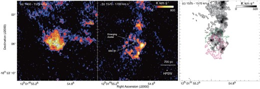
(a) Spatial distribution of the blueshifted cloud. The integration velocity range is VLSR = 1450–1525 km s−1. The contour levels are 300, 450, 600, 750, 900, 1060, 1070, and 1090 K km s−1. (b) The spatial distribution of the redshifted cloud. The integration velocity range is VLSR = 1570–1700 km s−1. (c) Intensity map of 12CO(J = 3–2) consisting of three velocity components. The black image indicates bridge features (VLSR = 1525–1570 km s−1). The red and green contours indicate the redshifted and blueshifted clouds, respectively. The contour levels of three velocity components are 40σ (95 K km s−1 for the bridge, 156 K km s−1 for the redshifted cloud, and 120 K km s−1 for blueshifted cloud). The symbols are the same as in figure 1. (Color online)
Figure 3 shows the distributions of the first and second moments toward SSC B1 in the velocity range of 1450–1700 km s−1. Figures 3a and 3b show the intensity-weighted velocity (first moment) and the velocity dispersion (second moment), respectively. There are two velocity components at ∼1450 km s−1 (green) and ∼1600 km s−1 (red). Figure 3b shows that the velocity dispersion is enhanced to 30–80 km s−1 where the redshifted and blueshifted clouds are overlapped as shown in figure 2c.
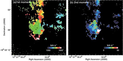
(a) First-moment map of 12CO(3–2) toward SSC B1. The velocity range VLSR = 1350–1650 km s−1 is used for calculation. (b) Second-moment map of 12CO(3–2) toward SSC B1. The same velocity range is used for calculation. The symbols are the same as in figure 1. (Color online)
In figures 4a, 4b, and 4c, the average velocity and velocity dispersion of the blueshifted cloud are 1510 km s−1 and 15 km s−1, respectively, those of the redshifted cloud are 1600 km s−1 and 30 km s−1, respectively, and those of the bridge are 1536 km s−1 and 7 km s−1, respectively. The velocity dispersions of the blueshifted and redshifted clouds are enhanced toward the western part of the cloud where two velocity clouds overlap as shown in figures 4c and 4d. Using the average velocity and dispersion, we found the two velocity ranges to be 1450–1525 km s−1 and 1570–1700 km s−1 for the two components.
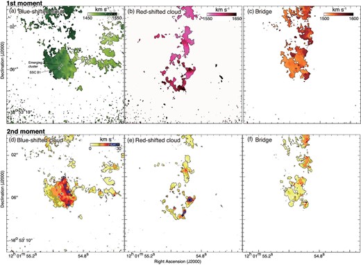
(a)–(c) First-moment map of 12CO(3–2) toward SSC B1. The velocity ranges used for calculating momentum are VLSR = 1450–1525 km s−1 (blueshifted cloud) for panel (a), VLSR = 1570–1700 km s−1 (redshifted cloud) for panel (b), and VLSR = 1525–1570 km s−1 (bridge) for panel (c). (d)–(f) Second-moment map of 12CO(3–2) toward SSC B1. Velocity ranges used for calculating moment are the same as in panels (a), (b), and (c). The symbols are the same as in figure 1. (Color online)
We calculated the cloud mass of the region enclosed by a contour of 20% of the peak integrated intensity using the CO-to-H2 conversion factor XCO = 0.6 × 1020 cm−2 (K km s−1)−1 (Zhu et al. 2003; Kamenetzky et al. 2014). The column density of molecular hydrogen N(H2) is calculated by the relationship N(H2) = XCO × WCO, where WCO is the integrated intensity of the 12CO(J = 1–0). The 12CO(J = 3–2) to 12CO(J = 1–0) integrated intensity ratio is taken to be 0.5 ± 0.1 for SGMC 4/5 (Ueda et al. 2012).
The molecular masses of the blueshifted cloud within an area enclosed by a contour of 219 K km s−1 (20% of the peak integrated intensity) and the redshifted cloud within an area enclosed by a contour of 173 K km s−1 (20% of the peak integrated intensity) are (4.0–6.0) × 107 M⊙ and (1.6–2.4) × 107 M⊙, respectively. The smaller and larger values of mass correspond to 12CO(J = 3–2) to 12CO(J = 1–0) integrated intensity ratios of 0.4 and 0.6, respectively. We also calculated the mass of the bridge component (VLSR = 1525–1570 km s−1) to be (5.2–7.8) × 107 M⊙ in the same way as for the blueshifted and redshifted clouds. We define the bridge component as the molecular cloud with VLSR of 1525–1570 km s−1 within a radius of 200 pc from SSC B1 because the emission in the same velocity range outside of the SGMC 4/5 is not related to cluster formation as shown in figure 2c. The bridge component extends northward, so the mass within a radius of 200 pc from B1 is (1.7–2.5) × 107 M⊙. Thus, the total mass of the redshifted, blueshifted, and bridge clouds around B1 is (7.3–10.9) × 107 M⊙. The error of the molecular mass is calculated via the uncertainty of the 12CO(J = 3–2) to 12CO(J = 1–0) ratio and the rms noise levels of 12CO(J = 3–2). In addition, the value of XCO possibly changes from 0.2 × 10²⁰ to 1.2 × 1020 cm−2 (K km s−1)−1 because of the difference of the relative abundance of CO to H2.
Figure 5 shows a comparison of the CO distribution with optical and near-infrared images of HST (B band, V band, I band, and Hα). The image shows two point-like sources (SSC B1 and the emerging cluster classified by Whitmore et al. 2014) as indicated by two crosses in figure 5a. SSC B1 and the emerging cluster correspond to the southern black cross and the northern cross, respectively. The two sources correspond to two intensity depressions of the blueshifted cloud (figure 5a), and the cavity of the redshifted cloud corresponds to the extended emission (gray dashed circle in figure 5b). The images in figures 5c and 5d are the Hα
emission, and the correspondence of the extended emission and the cavity of the redshifted cloud is remarkable. A typical radius of the cavity is ∼120 pc, which is about the same size as the blueshifted cloud. The correspondence shows that the two clouds are physically associated with SSC B1 and are the parent clouds of SSC B1.
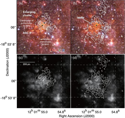
(a), (b) False color image toward SGMC 4/5 obtained with HST overlaid with integrated intensity distribution of12CO(J = 3–2) for the blueshifted cloud and redshifted cloud by contours. The B-band image is shown in blue, V-band image in green, and a combination of the I-band and Hα images in red. The integrated velocity ranges are the same as in figure 2. The contour levels are 300, 450, 600, 750, 900, 1060, 1070, and 1090 K km s−1 for panel (a); 120, 220, 320, 420, 520, 620, 720, 820, 920, and 1020 K km s−1 for panel (b). (c), (d) Integrated intensity distribution of 12CO(J = 3–2) for the blueshifted cloud and the redshifted cloud by contours superposed on the Hα image obtained with HST. The integrated velocity ranges and contour levels of panels (c) and (d) are the same as in panels (a) and (b). The symbols are the same as in figure 1. (Color online)
Whitmore et al. (2014) classified the emerging cluster as a separated object for the first time. Whitmore et al. (2014) defined the five evolutionary classifications of the SGMCs. Based on the previous study of the GMC evolution model in the Local Group of galaxies (LMC: Fukui et al. 1999; Kawamura et al. 2009; M 33: Miura et al. 2012), Whitmore et al. (2014) extended the classification to older clusters with no CO using radio continuum and optical/near-infrared data in addition to CO. The emerging cluster is classified as stage 3 (time scale: 0.11 Myr) and gas and dust are removed. Thanks to the higher angular resolution, we find the intensity depression toward the emerging cluster, which we did not find in Paper I. Thus, it is likely that the two clouds are also associated with the emerging cluster.
3.2 Complementary distribution and bridge features
Figure 6 shows an overlay of the distributions of the two velocity components from the present analysis, the theoretical simulation result, and a schematic of the two clouds. According to the previous works, in two colliding clouds which show a complementary distribution, we often find a displacement between them (e.g., Fukui et al. 2018; Takahira et al. 2014), which is a general signature for a collision the velocity of which makes an angle not close to either 0° or 90°. Takahira, Tasker, and Habe (2014) made hydrodynamical numerical simulations of two spherical clouds with different radii in a head-on collision. In the collision the small cloud creates a cavity that is the size of the small cloud in the large cloud. The cavity should have a distribution that is complementary to the small cloud. Fukui et al. (2018) presented synthetic observations of such a collision using the results of Takahira, Tasker, and Habe (2014), and showed that the complementary distribution usually has a displacement in the sky because of the projection effect of the collision path which makes a certain non-zero angle to the line of sight.
Following the algorithm by Fujita et al. (2021), we moved the redshifted cloud from the original position over ±90 pc in a step of 1.8 pc (size of pixel) step in the two orthogonal directions of RA and Dec, and calculated the correlation coefficient with the integrated intensity of the blueshifted cloud for each pixel. We calculated Spearman’s correlation coefficient between the integrated intensities of two velocity components, and looked for the position where the correlation coefficient is at its minimum. The method is appropriate when the feedback is not significant and the shapes of the two clouds are well kept after the collision. In figure 6a we see the two clouds exhibit a complementary distribution with a possible displacement. Figure 6b shows the result after a displacement of 70 pc in length and at a position angle of 126°. These parameters give the minimum correlation coefficient of −0.7, and their coincidence looks good. Figure 6c shows a schematic of two clouds before, during, and after the collision, modified from figure 14 in Paper I. In figure 6d shows the two different radii clouds whose colliding direction is the line of sight (Takahira et al. 2014).
4 Discussion
4.1 Collision picture toward SSC B1
Paper I suggested that the two clouds are colliding toward SSC B1 based on the complementary distribution and bridge features of the ALMA Cycle 0 data. The present analysis of the Cycle 3 data with four-times-higher resolution showed significant details of the complementary distribution and the bridge features of the two clouds, allowing us to elaborate the collision picture. In particular, a displacement of 70 pc at a position angle of |${126^{\circ}}$| was derived by the fitting procedure between the small cloud and the cavity of the large cloud (Fujita et al. 2021; see also Fukui et al. 2018).
The new collision picture above helps to estimate the collision parameters better. The collision time scale is calculated by a ratio of the traveled distance ∼70 pc divided by the collision velocity ∼100 km s−1, giving 0.7 Myr. The time scale is valid if the collision angle is 45°. If the collision direction makes an angle of 30° or 60° to the line of sight, the time scale can vary from 0.4 to 1.4 Myr corrected for the projection. This value is consistent with the estimated cluster age, 1–3.5 Myr (Gilbert & Graham 2007; Whitmore et al. 2010).
According to figure 6, the blueshifted small cloud collided close to the center of the redshifted large cloud, where the small cloud moved from the south to the north and fully passed through the large cloud. As a result, the collision could have created the cavity in the large cloud, and compressed the interface layer between the two clouds (see the schematic diagram in figure 6). Part of the remnant of the interface layer is seen as the bridge stellar objects (figure 2c), while the rest of the gas has been ionized. The near-infrared bright and compact features in both clouds correspond to the intensity depressions toward the stellar objects and the associated extended feature. This suggests that part of the two clouds is converted to the stars of the cluster in the collision.
4.2 Mass budget and star formation efficiency
We estimate the mass budget and the star formation efficiency in the two colliding clouds by considering the gas mass, stellar mass, and ionized gas mass, and extrapolating the gas mass of the parental cloud before formation.
4.2.1 Mass budget
We attempt to estimate the star formation efficiency in the colliding clouds. Figure 2 shows that the two clouds are clearly separated with a displacement of 70 pc. We adopt an XCO factor of 0.6 × 1020 cm−2 (K km s−1)−1 which has some large uncertainty (Zhu et al. 2003; Kamenetzky et al. 2014), and the uncertainty in the molecular mass is mainly due to XCO. For the XCO masses of redshifted cloud and the blueshifted cloud are |$2.0^{+0.4}_{-0.4} \times 10^{7}$|M⊙ and |$5.0^{+1.0}_{-1.0} \times 10^{7}$|M⊙, respectively, where only the error bars in an intensity ratio of the J = 3–2 and 1–0 transitions are considered. Figure 5 shows that the formation of the two clusters, SSCB1 and the emerging cluster, is taking place in the blueshifted cloud, as evidenced by the two depressions of the molecular gas accompanying the Hα emission. The blueshifted cloud has two additional molecular peaks outside the two clusters, which are suggested by Whitmore et al. (2014) to be two more candidate protoclusters as indicated in figure 5, whereas they have no stellar emission. The gas masses of the protocluster candidates ALMA 4 and ALMA 5 are calculated to be 2.0 × 10⁶ M⊙ and 3.4 × 10⁶ M⊙ above integrated intensity levels of 633 K km s−1 and 774 K km s−1, which correspond to 50% of the peak integrated intensity, respectively. The sizes of ALMA 4 and ALMA 5 are 18 pc and 21 pc in radius, respectively.
In order to estimate the molecular mass which formed the two clusters SSC B1 and the emerging cluster, we interpolate the mass which existed in the two cavities prior to the collision. It is probable that the molecular gas is depleted by the cluster formation and the resultant ionization. We assume that the radius R of the parent cloud of SSC B1 and the emerging cluster is the geometric mean of R of the two protocluster candidates. We estimate R of the depressions to be ∼19 pc for SSC B1 and the emerging cluster. We assumed that the initial |$N_{\rm H_{2}}$| toward SSC B1 prior to the cluster formation is equal to an average of the peak |$N_{\rm H_{2}}$| toward the two protocluster candidates ALMA4 and ALMA5. Then, the parent cloud mass Mparent is given by [(the average |$N_{\rm H_{2}}$| of ALMA4 and ALMA5) − (the present |$N_{\rm H_{2}}$| toward SSC B1)] × πR2. We estimate the molecular mass inside the radius to be |$3.4^{+3.4}_{-2.3} \times 10^{6}$|M⊙. A similar method is applied to the emerging cluster and we estimate the radius of the parent cloud to be 19 pc for the emerging cluster, and find that the mass in the radius is |$3.8^{+3.8}_{-2.5} \times 10^{6}$|M⊙. The relevant figures are listed in table 1.
Physical properties of the parent cloud of the clusters.*
| Object | WCO [K km s−1]† | LHα | R | Mparent‡ | |$M_{\rm H}$|ii | Mcluster |
|---|---|---|---|---|---|---|
| |$N_{\rm H_{2}}$| [1022 cm−2]† | [1038 erg s−1] | [pc] | [106 M⊙] | [106 M⊙] | [106 M⊙] | |
| (1) | (2) | (3) | (4) | (5) | (6) | (7) |
| SSC B1 | 3.6 | 11 | 19 | 3.4|$^{+3.4}_{-2.3}$| | ∼1.9 | 6.8 |
| 303 | ||||||
| Emerging cluster | 2.2 | 2.4 | 19 | 3.8|$^{+3.8}_{-2.5}$| | ∼0.4 | — |
| 187 | ||||||
| Protocluster candidate | 15 | — | 18 | 2.0|$^{+2.0}_{-1.3}$| | — | — |
| ALMA 4 | 1266 | |||||
| Protocluster candidate | 19 | — | 21 | 3.4|$^{+3.4}_{-2.3}$| | — | — |
| ALMA 5 | 1548 |
Column (1): Object name. Column (2): Column density and integrated intensity of molecular cloud. Column (3): Luminosity of Hα emission obtained with HST (Whitmore et al. 2010). Column (4): The radius of the object. The radius of the protocluster is defined as the size where the integrated intensity decreases to 50% of the peak integrated intensity. Radii of parent clouds of SSC B1 and the emerging cluster are assumed to be geometric means of radii of the two protoclusters. Column (5): Mparent is molecular mass inside of the radius projected to have been within the radius based on extrapolation from ALMA4 and ALMA5. The CO cloud masses of SSC B1 and the emerging cluster are given by [(the average |$N_{\rm H_{2}}$| of ALMA4 and ALMA5) − (the present |$N_{\rm H_{2}}$| toward SSC B1|$/$|emerging cluster)] × πR2. Column (6): Ionized gas mass derived by using the relationship between Hα luminosity and ionized gas mass |$M_{\rm gas \ ionized} = 0.98\times 10^{9} (\frac{L_{\rm H\alpha }}{10^{43}\:\mbox{erg}\:\mbox{s}^{-1}}) {(\frac{n_{\rm e}}{100\:\mbox{cm}^{-3}})}^{-1}$| (Osterbrock & Ferland 2006). LHα is the luminosity of Hα [erg s−1] and ne is assumed to be 100 cm−3. Column (7): Total stellar mass of the cluster (Whitmore et al. 2010).
Minimum value for SSC B1 and the emerging cluster, and maximum value for the protocluster candidates.
Errors of Mparent are derived from three times uncertainty of XCO factor.
Further, we use the Hα emission to calculate the ionized gas mass by adopting the following relationship Mgas ionized = 0.98 × 10⁹(LHα/1043 erg s−1)(ne/100 cm−3)−1, where LHα is the luminosity of Hα in units of erg s−1 and ne is the averaged electron density in units of cm−3 (Osterbrock & Ferland 2006). We assume ne to be 100 cm−3 from the size–density relation of extragalactic H ii regions (Hunt & Hirashita 2009). The values of LHα of SSC B1 and the emerging cluster are estimated to be 1.1 × 1039 erg s−1 and 2.4 × 1038 erg s−1, respectively, and we calculate that the ionized gas masses of SSC B1 and the emerging cluster are 2 × 10⁶ M⊙ and 0.4 × 10⁶ M⊙, respectively. These are an order of magnitude smaller than the molecular mass, at most.
4.2.2 Star formation efficiency
The cluster mass of SSC B1 is estimated to be 6.8 × 10⁶ M⊙ (Whitmore et al. 2010) and 4.2 × 10⁶ M⊙ (Gilbert & Graham 2007). The former is corrected for the extinction and we adopt it in what follows. The peak luminosity of Hα of SSC B1 is greater by an order of magnitude than that of the emerging cluster. This suggests that the emerging cluster is young and has not yet ionized its surrounding gas. The cluster mass of the emerging cluster therefore must be crude at best. Table 1 lists WCO and the extrapolated parent cloud mass of the two clusters and two protoclusters.
Except for SSC B1, there is no reliable estimate of the cluster mass, and we focus on SSC B1. Using the cluster mass and the extrapolated molecular mass, we estimate the star formation efficiency (SFE) to be a ratio of the cluster mass divided by the total mass of extrapolated molecular mass and ionized gas mass, 6.8 × 10⁶ M⊙/[(3.0–8.7) × 106 M⊙] ∼ 0.78, if we assume an XCO value ranging from 0.2 × 10²⁰ to 1.2 × 10²⁰ depending on the difference of the relative abundance of CO to H2 (Zhu et al. 2003). We assume that the relative abundance of CO to H2 possibly changes from 5 × 10⁻⁵ to 2.7 × 10⁻⁴ by observations of GMCs in the star-forming regions of the Milky Way and the theoretical model (e.g., Blake et al. 1987; Farquhar et al. 1994). Obviously, SFE greater than 1 does not make sense. One interpretation of this extremely high SFE is that the calculation of the extrapolated parental cloud mass is too small. This suggests that the column density of the parental cloud was larger than the column density of these other proto-clusters. We infer that the local cluster formation within 20 pc in radius is taking place at very high SFE, more than 0.78. Over the whole collision process, the total molecular mass of the blueshifted cloud is ∼2 × 10⁸ M⊙ on a 200–300 pc scale, and SFE for SSC B1 becomes only |$\sim\! 3\%$|. If we include the mass of the emerging cluster and the two protocluster candidates, the total SFE becomes |$\sim\! 12\%$| under an assumption of their equal cluster mass. Thus, the cloud–cloud collision may not be an extremely efficient process in converting the cloud mass into clusters in the SGMC 4–5 region.
4.3 SSC formation and physical condition of around environment
It is suggested that the high-pressure environment is a requirement for the SSC formation (Elmegreen 1989; Elmegreen & Efremov 1997). Johnson et al. (2015) and Finn et al. (2019) found the high-pressure environment in the overlap region. Furthermore, Paper I revealed a positive correlation between the compressed gas pressure generated by collision and total stellar mass of cluster. The typical pressure of the colliding clouds is estimated to be (1.7–8.0) × 108 K cm−3 by using the relationship |$P_{\rm e}= ({3\Pi \it M v^{2}})/({4 \pi R^{3}}) = \rho _{\rm e} v^{2}$|, which is consistent with the relationship derived by Paper I. M is the cloud mass, v is the colliding velocity (difference of peak velocity of colliding clouds), R is the radius of the cloud, and ρe is the density at the cloud edge. Π is defined by ρe = Πρ, where ρ is the mean density in the cloud. We adopt Π = 0.5 (Johnson et al. 2015; Finn et al. 2019). The error in the external pressure mainly consists of the uncertainty of the mass estimation and the projection effect on the collision velocity. If we assume that an angle of the collision path to the line of sight θ is 30°–60°, the collision velocity could range from ∼115 to ∼200 km s−1. For θ = 90°, we do not see the two velocity components, and for θ = 0° we do not see the displacement between the two components as shown in figure 6.
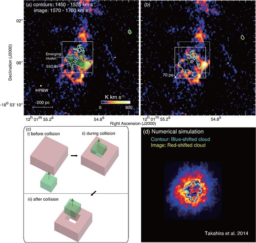
(a) CO intensity map of the blueshifted cloud by contours superposed on the redshifted cloud. The contour levels and symbols are the same as in figure 2b. (b) Same as panel (a), but the contour of the blueshifted cloud is displaced. The contour level is 300 K km s−1. The projected displacement is 70 pc with a position angle of 126°. (c) The panel shows rectangular solid model clouds before the collision (i), during the collision (ii), and after the collision (iii) for SGMC 4/5. Panels (a) and (b) correspond to (iii) and (ii), respectively. (d) Result of synthetic observation based on the numerical simulation by Takahira, Tasker, and Habe (2014). Contour and image indicate the blueshifted and redshifted clouds, respectively. (Color online)
Feedback is believed to be important in high-mass star formation. The present results reveal some novel aspects of the feedback. Figure 4 shows the distribution of the first moment and the second moment of the blueshifted, redshifted, and bridge clouds. The stellar objects in the cluster are plotted by crosses, and no variation of the average velocity or velocity dispersion is seen, suggesting that the stellar feedback is not appreciably affecting the gas dynamics. Figure 3 also shows the spatial distribution of the first moment and second moment in the whole velocity range (VLSR). The velocity dispersion is raised to ∼15 km s−1 toward the stellar objects, which is possibly induced by stellar feedback on several tens of pc scale. On the other hand, the maximum velocity dispersion is ∼80 km s−1 in the area where the redshifted cloud and the blueshifted cloud are overlapped. From these results, it is natural to understand the velocity structures of the whole SGMC 4/5 by the motion of the redshifted and blueshifted clouds, not by feedback.
We suggest that the velocity distribution of the clouds is more influenced by the collisional interaction than the feedback, as indicated by the enhancement of the second moment having a spatial gradient from the east to west which has no correlation with the stellar objects. The area of the cluster formation is strongly ionized by the forming stars in the cluster in both clouds, as depicted in figure 5. The present high resolution shows the cavity is fully enclosed by the large cloud (see figure 6).
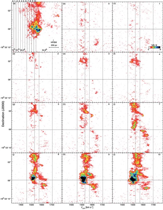
Channel maps of declination–velocity diagrams. (a) Total integrated intensity map of SGMC 4/5. The integration velocity range is the same as in figure 1b. Dashed vertical lines indicate the integration ranges of declination–velocity diagrams in RA. (b)–(l) Declination–velocity diagrams of 12CO (J = 3–2). The upper right-hand number denotes the integration range in panel (a). (Color online)
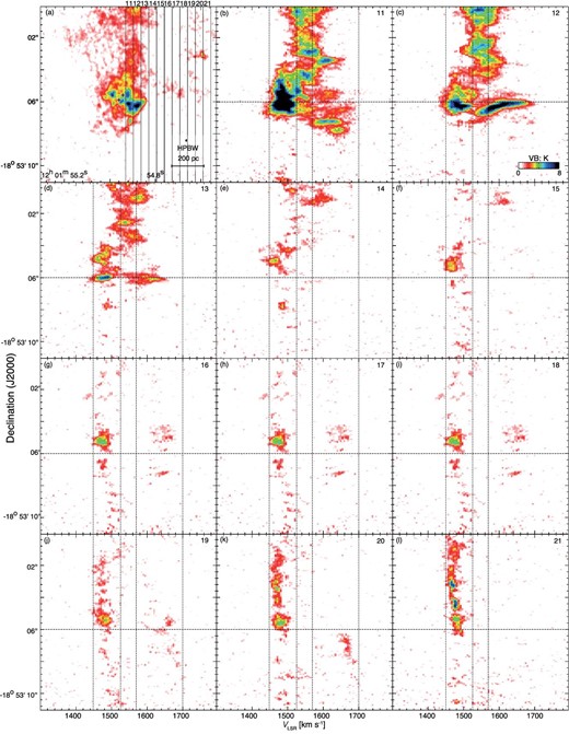
Channel maps of declination–velocity diagrams. (a) Total integrated intensity map of SGMC 4/5. The integration velocity range is the same as in figure 1b. Dashed vertical lines indicate the integration ranges of declination–velocity diagrams in RA. (b)–(l) Declination–velocity diagrams of 12CO (J = 3–2). The upper right-hand number denotes the integration range in panel (a).
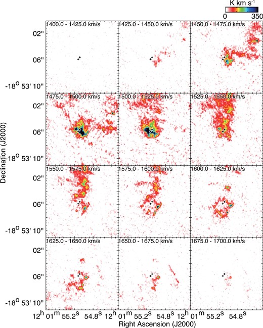
Velocity channel maps of 12CO(3–2) toward the SGMC 4/5 with a velocity step of 25 km s−1. The symbols are the same as in figure 1.
5 Conclusion
The Antennae Galaxies are the most outstanding major merger closest to the Milky Way. We analyzed the ALMA Cycle3 dataset of the 12CO(J = 3–2) emission towards the SSC B1 and derived the molecular distribution at 10 pc resolution. The main conclusions of the present study are summarized as follows:
The present results confirm that the molecular gas in SSC B1 has two velocity peaks, at 1500 km s−1 and 1600 km s−1 (Paper I). The spatial distributions of the clouds resolved with a resolution of 10 pc shows a complementary distribution with a displacement of 70 pc, which was determined more accurately than in Paper I. The two clouds are connected with bridge features in the intermediate velocity range. The complementary distribution matches well the numerical simulation by Takahira, Tasker, and Habe (2014).
The SFE of SSC B1 is estimated to be larger than ∼0.78 by the total mass including the extrapolated molecular mass and ionized gas at 20 pc. The SFE is very high on the 20 pc scale. On the other hand, over the whole collision process, the total mass of the blueshifted cloud associated with the cluster formation is ∼2 × 10⁸ M⊙ on the 200–300 pc scale, and SFE is only |$\sim\! 3\%$|. If we include the total stellar mass of the emerging cluster and two protocluster candidates, the SFE becomes |$\sim\! 12\%$| on the assumption of their equal cluster mass. Thus, the cloud–cloud collision may not be an extremely efficient process in the SGMC 4–5 region.
The velocity distribution in the two CO clouds are derived as the first moment and second moment, and are compared with compact near-infrared sources and the Hα image. The result shows that the gas motion has no sign of the velocity field being perturbed by stellar sources (e.g., stellar radiation and wind). We therefore argue that significant kinematic feedback by the newly formed stars is not important, except for the ionization which probably evacuated the molecular gas. We found two cavities formed by the ionization of clusters and estimated ionized gas mass was ∼(0.4–1.9) × 106 M⊙. This suggests that the cloud kinematics is dominated by the galactic tidal interaction.
Acknowledgements
This paper makes use of the following ALMA data: ADS/ JAO.ALMA #2011.0.00876, and #2015.1.00038.S. ALMA is a partnership of the European Southern Observatory (ESO), National Science Foundation (NSF), National Institutes of Natural Sciences (NINS), National Research Council of Canada (NRC), Ministry of Science and Technology (MOST), and Institute of Astronomy and Astrophysics, Academia Sinica (ASIAA). The Joint ALMA Observatory is operated by the ESO, Associated Universities, Inc. (AUI)/National Radio Astronomy Observatory (NRAO), and National Astronomical Observatory of Japan (NAOJ). This paper is also based on observations made with the NASA/ESA Hubble Space Telescope, obtained from the data archive at the Space Telescope Science Institute. STScI is operated by the Association of Universities for Research in Astronomy, Inc. under NASA contract NAS 5-26555. K. Tsuge was supported by the ALMA Japan Research Grant of NAOJ ALMA Project, NAOJ-ALMA-232. This study was supported by JSPS KAKENHI Grant Numbers JP15H05694, JP18K13582, JP19K14758, and JP19H05075. We would like to thank the referees for their constructive inputs.
Appendix 1 CO channel maps of position diagrams
We show the 21 declination–velocity diagrams of the 12CO(J = 3–2) in figures 7 and 8. The integration range is |${0{^{\prime \prime }_{.}}5}$| (∼54 pc), and the integration range is shifted from east to west in |${0{^{\prime \prime }_{.}}5}$| step.
Appendix 2 Velocity channel maps
We show the velocity channel maps of the 12CO(J = 3–2) of SGMC 4/5 in figure 9. The velocity range is between 1400 and 1700 km s−1.
