


Abstract
In this paper, we present the results from spectroscopic and photometric observations of the M-type flare star YZ CMi in the framework of the Optical and Infrared Synergetic Telescopes for Education and Research (OISTER) collaborations during the Transiting Exoplanet Survey Satellite (TESS) observation period. We detected 145 white-light flares from the TESS light-curve and four Hα flares from the OISTER observations performed between 2019 January 16 and 18. Among them, three Hα flares were associated with white-light flares. However, one of them did not show clear brightening in the continuum; during this flare, the Hα line exhibited blue asymmetry which lasted for ∼60 min. The line-of-sight velocity of the blueshifted component is in the range from −80 to −100 km s−1. This suggests that there can be upward flows of chromospheric cool plasma even without detectable red/near-infrared (NIR) continuum brightening. By assuming that the blue asymmetry in the Hα line was caused by a prominence eruption on YZ CMi, we estimated the mass and kinetic energy of the upward-moving material to be 1016–1018 g and 1029.5–1031.5 erg, respectively. The estimated mass is comparable to expectations from the empirical relation between the flare X-ray energy and mass of upward-moving material for stellar flares and solar coronal mass ejections (CMEs). In contrast, the estimated kinetic energy for the non-white-light flare on YZ CMi is roughly two orders of magnitude smaller than that expected from the relation between flare X-ray energy and kinetic energy for solar CMEs. This could be understood by the difference in the velocity between CMEs and prominence eruptions.
1 Introduction
Solar flares are sudden and energetic explosions in the solar atmosphere around sunspots. Flares are observed in all wavelength bands from radio to high-energy gamma-rays. They are thought to be the rapid releases of magnetic energy through magnetic reconnection in the solar corona (e.g., Shibata & Magara 2011 and references therein). Part of the energy released by the magnetic reconnection is transported from the reconnection site into the chromosphere via thermal conduction and high-energy particles, which causes heating, produces line emission (e.g., Hα), and can even produce hard X-ray and optical continuum emission. This intense heating of chromospheric plasma is thought to cause the upward flow of plasma called chromospheric evaporation (Fisher et al. 1985).
Similar periods of rapid increases and slow decays of intensity in radio, optical, and X-ray bands are also observed on various types of stars, and they are called stellar flares. In particular, it is known that young stellar objects, close binary systems, and M-type main sequence stars (dMe stars) exhibit frequent and energetic flares (e.g., Shibata & Yokoyama 2002; Gershberg 2005; Reid & Hawley 2005; Benz & Güdel 2010; Hawley et al. 2014; Linsky 2019; Namekata et al. 2020b). Because of the similarity in observational properties between stellar flares and solar flares (e.g., Nuepert effect in solar/stellar flares; Neupert 1968; Dennis & Zarro 1993; Hawley et al. 1995; Guedel et al. 1996), they are considered to be caused by the same physical processes (i.e., plasma heating by accelerated particles and evaporation). Many spectroscopic studies of superflares have been carried out in order to understand the dynamics of plasma during flares and the radiation mechanisms of flares. Various spectroscopic observations of solar flares have shown that chromospheric lines (e.g., Hα, Ca ii, Mg ii) often exhibit asymmetric line profiles during flares. Red asymmetries (enhancement of the red wing) have been observed frequently during the impulsive phase of the flares (e.g., Švestka et al. 1962; Ichimoto & Kurokawa 1984; Canfield et al. 1990; Shoji & Kurokawa 1995; Berlicki 2007; Kuridze et al. 2015; Kowalski et al. 2017; Graham et al. 2020). This is thought to be caused by the chromospheric condensation, which is the downward flow of cool plasma in the chromosphere. Blue asymmetries (enhancement of the blue wing) have also been observed mainly in the early phase of flares (e.g., Švestka et al. 1962; Canfield et al. 1990; Heinzel et al. 1994b; Kuridze et al. 2016; Tei et al. 2018; Huang et al. 2019). It is suggested that blue asymmetry is caused by an upflow of cool plasma, which is lifted up by expanding hot plasma owing to the deep penetration of non-thermal electrons into the chromosphere during a flare (Tei et al. 2018; Huang et al. 2019). However, the detailed origins of these blue asymmetries are still controversial.
Similar line asymmetries in chromospheric lines (especially Hα) have been observed during stellar flares. In addition to red asymmetries (e.g., Houdebine et al. 1993), various blue asymmetries have been widely observed (e.g., Houdebine et al. 1990; Gunn et al. 1994; Fuhrmeister et al. 2008; Vida et al. 2016; Honda et al. 2018; Muheki et al. 2020). Vida et al. (2016) reported several Hα flares on the M4 dwarf V374 Peg showing blue asymmetries with a line-of-sight velocity ranging from −200 to −400 km s−1. They also found that red-wing enhancements in the Hα line were observed after blue asymmetries, which suggest that the erupted cool plasma fell back on the stellar surface. Honda et al. 2018 reported a long-duration Hα flare on the M4.5 dwarf EV Lac. During this flare, a blue asymmetry in the Hα line with the dipolar velocity of ∼−100 km s−1 has been observed for >2 hr. Since we cannot obtain the spatially resolved information for stellar flares, the line-of-sight motions of cool plasma such as coronal rains, surges, and filament/prominence eruptions may also cause red/blue asymmetries. For example, if the cool plasma is launched upward and seen above the limb, the emission can cause blueshifted or redshifted enhancements of the Hα line (e.g., Odert et al. 2020). As observed on the Sun, such eruptions (surges and filament/prominence eruptions) can evolve into CMEs (coronal mass ejections) if the erupted plasma is accelerated and the velocity exceeds the escape velocity (e.g., Gopalswamy et al. 2003; Shibata & Magara 2011, and reference therein).
Other studies have suggested that blue asymmetries in chromospheric lines may be due to stellar mass ejections. Vida et al. (2019) reported a statistical analysis of 478 stellar events with asymmetries in Balmer lines of M-dwarfs, which were found from more than 5500 “snapshot” spectra (cf. similar events were also reported from other snapshot data in Fuhrmeister et al. 2018). The velocity and mass of the possible ejected materials estimated from the blueshifted or redshifted excess in Balmer lines range from 100–300 km s−1 and 1015–1018 g, respectively. Moschou et al. (2019) presented the correlations between the mass/kinetic energy of CMEs and the X-ray energy of associated flares on various types of stars. They found that estimated stellar flare CME masses are consistent with the trends extrapolated from solar events but kinematic energies are roughly two orders of magnitude smaller than expected. It is important to understand the properties of stellar CMEs in order to evaluate effects of stellar activities not only on the mass and angular momentum loss of the star (e.g., Osten & Wolk 2015; Odert et al. 2017; Cranmer 2017), but also on the habitability (e.g., loss of atmosphere, atmospheric chemistry, climate, radiation dose) of exoplanets (e.g., Lammer et al. 2007; Linsky 2019; Segura et al. 2010; Tilley et al. 2019; Scheucher et al. 2018; Airapetian et al. 2020, Yamashiki et al. 2019). However, our understanding of asymmetries in chromospheric lines and their connections with stellar flares/CMEs is still limited by the low number of samples observed in time-resolved spectroscopy simultaneously with high-precision photometry.
In order to investigate the connection between the blue/red asymmetries in the Hα line and the properties of flares, we conducted photometric and spectroscopic observations of an active M dwarf, YZ CMi, during the Transiting Exoplanet Survey Satellite (TESS; Ricker et al. 2015) observation window (Sector 7: from 2019 January 07 to 2019 February 01). In this paper, we report on results from the statistical analysis of flares on YZ CMi from the TESS light-curve and photometric and spectroscopic observations in the framework of the Optical and Infrared Synergetic Telescopes for Education and Research (OISTER; M. Yamanaka et al. in preparation). The details of our observations and analysis are described in section 2. We present the properties of detected flares from TESS and OISTER observations in section 3. In section 4, we discuss (1) the differences between Hα flares with and without white-light flares, (2) blue asymmetry observed during the Hα flare without a white-light flare, (3) the rotational modulations observed in the continuum and Hα emission line, and (4) the statistical properties of flare duration.
2 Data and methods
2.1 Target star: YZ CMi
YZ CMi (= Gl 285 = Ross 882) is a well-known 11 mag M4.5Ve flare star, whose distance from the Earth is about 5.99 pc (Gaia Collaboration 2018). Flares on YZ CMi were first discovered at optical wavelengths by van Maanen (1945) and were later detected at radio wavelengths (Lovell 1969; Spangler et al. 1974) and X-ray wavelengths (Grindlay & Heise 1975). Frequent stellar flares have been observed on YZ CMi in several wavelength ranges (Lacy et al. 1976; Mitra-Kraev et al. 2005; Kowalski et al. 2013), and in particular, a large superflare whose U-band energy is larger than 1034 erg is reported in Kowalski et al. (2010). Zeeman-broadening measurements suggest the existence of strong magnetic fields on the stellar surface (e.g., Johns-Krull & Valenti 2000; Reiners & Basri 2007). According to Zeeman–Doppler Imaging observations, the visible pole of YZ CMi is covered by a strong spot with a radial magnetic field strength of up to 3 kG (Morin et al. 2008).
2.2 Flare detection from the TESS light-curve
We analyzed the TESS Sector 7 Pre-search Data Conditioned Simple Aperture Photometry (PDC-SAP) light curve (Vanderspek et al. 2018; Fausnaugh et al. 2019) of YZ CMi retrieved from the MAST Portal site.1 In order to detect small flares, we first removed non-flare signals such as long-term trend and rotational brightness variations from the light curve and then searched for flares. Since there is a data gap between BJD 2458503.04 and 2458504.71 in the TESS light-curve (figure 1), we divided the whole TESS light-curve into two subsets (BJD 2458491.64–2458503.04 and BJD 2458504.71–2458516.09), and analyzed each light curve subset separately. First we removed some of the large flares from the light curve beforehand since large flares with long flare duration affect the long-term light-curve fitting process. The initial flare detection was performed with the same method used in our previous studies (Maehara et al. 2012; Shibayama et al. 2013). The excluded data points in the light curve were interpolated using “interpolate.Akima1DInterpolator” in the Python Scipy package. After removing flares and interpolation of the removed data points, we extracted the long-term trend and rotational variations using the fifth-order Bessel filter in the SciPy signal module. We used the cut-off frequency of 0.2 d−1 in this process. Then we removed the extracted signal from the light curves. We selected the data points which satisfied the following conditions as the flare candidates: (1) the residual brightness of the data point is higher than the upper |$10\%$| of the residual light curve, (2) at least two consecutive data points exceed the flare detection threshold, (3) the decay time is longer than the rise time. Finally, we checked all the light curves of flare candidates by eye and eliminated the misidentified candidates. The total number of the automatically selected flare candidates is 194 and the number of confirmed flares is 145. A table of the flares identified in TESS [with peak time, flare amplitude normalized by the average stellar brightness, equivalent duration (the model-independent energy in units of seconds; Gershberg 1972), bolometric energy of flare, and flare e-folding time] is provided in the supplementary data section available online.
![(a) Light curve of YZ CMi observed with TESS, covering the times of OISTER and APO observations. The horizontal and vertical axes represent the observation time in Barycentric Julian Date (BJD) and relative flux normalized by the average flux. The horizontal bars (red, green and blue) in panels (a) and (c) indicate the times of observations by MITSuME (g-, RC-, and IC-band photometry), HOWPol (low-resolution spectroscopy), and MALLS (medium-resolution spectroscopy), respectively. The horizontal bars (magenta and cyan) in panels (a) and (c) indicate g-band photometry with ARCSAT and high-resolution spectroscopy by ARCES at APO. Upward arrows below the light curve indicate the peak times of flares detected by our flare detection method. (b) Light curve of the largest flare on YZ CMi observed with TESS during the TESS Sector 7 (denoted by a downward arrow in panel a). The horizontal axis is the time from the flare peak [T0(BJD) =2458507.0233]. (c) Same as panel (a) but for the light curve around OISTER observations. (d) Same as panel (a) but for the light curve around APO observations. (Color online)](https://oup.silverchair-cdn.com/oup/backfile/Content_public/Journal/pasj/73/1/10.1093_pasj_psaa098/2/m_psaa098fig1.jpeg?Expires=1749099088&Signature=DPURXCSdYb0ePx08pxeUhfmXcm8WJha--bklz8it08uwivhnOOvxxozz~5COpPSs0tDl8JTr~VYvheFEDvufZie8-QYOewMut7vhUKSsResFOp6yjtGGLkG0U-aDEml5GuQIoa3Yes~x1RCdmpnnzqf3hd-3LjO8tukwgiJFZG9dOH0X7brkakvohiUWI6gCcg9Q8~O2zSHveg~oS0PGCfU0haqsynux9hl9AXmOI7GpJKCSdpgxHJWbBt8kjwWbrZ0X11hMoyVwY5ydZNpoyD675JOK2VSh4PDehS-nCT2OHq0wZXOG9Pvb-iRIoIcqpVOZPTPqe~d5VddkPPhKxQ__&Key-Pair-Id=APKAIE5G5CRDK6RD3PGA)
(a) Light curve of YZ CMi observed with TESS, covering the times of OISTER and APO observations. The horizontal and vertical axes represent the observation time in Barycentric Julian Date (BJD) and relative flux normalized by the average flux. The horizontal bars (red, green and blue) in panels (a) and (c) indicate the times of observations by MITSuME (g-, RC-, and IC-band photometry), HOWPol (low-resolution spectroscopy), and MALLS (medium-resolution spectroscopy), respectively. The horizontal bars (magenta and cyan) in panels (a) and (c) indicate g-band photometry with ARCSAT and high-resolution spectroscopy by ARCES at APO. Upward arrows below the light curve indicate the peak times of flares detected by our flare detection method. (b) Light curve of the largest flare on YZ CMi observed with TESS during the TESS Sector 7 (denoted by a downward arrow in panel a). The horizontal axis is the time from the flare peak [T0(BJD) =2458507.0233]. (c) Same as panel (a) but for the light curve around OISTER observations. (d) Same as panel (a) but for the light curve around APO observations. (Color online)
2.3 OISTER observations
We conducted the coordinated observing campaign of YZ CMi on 2019 January 16, 17, and 18 in the framework of OISETR collaboration. The log of the observation is summarized in table 1.
Log of OISTER and APO observations.
| Telescope/instrument | Start–end (UT) | Exp. time (s) | Number of data |
|---|---|---|---|
| MITSuME 0.5 m | 2019 January 16.625–16.793 | 5 | 590 (g), 608 (RC), 610 (IC) |
| (g, RC, IC-band) | 17.713–17.786 | 5 | 123 (g), 124 (RC), 124 (IC) |
| Okayama, Japan | 18.623–18.793 | 5 | 853 (g), 891 (RC), 895 (IC) |
| Kanata 1.5 m/HOWPol | 16.625–16.816 | 60 | 224 |
| (4000–9000 Å; λ/Δλ ∼ 400) | 17.667–17.740 | 60 | 77 |
| Hiroshima, Japan | 18.639–18.792 | 60 | 186 |
| Nayuta 2 m/MALLS | 16.604–16.801 | 250 | 54 |
| (6350–6800 Å; λ/Δλ ∼ 10000) | 18.629–18.793 | 250 | 51 |
| Hyogo, Japan | |||
| ARCSAT 0.5 m/flarecam | 26.131–26.423 | 4, 15, 30* | 310 (g) |
| (g-band) | 27.113–27.418 | 4 | 138 (g) |
| New Mexico, United States | 28.108–28.402 | 4, 6, 12, 20* | 155 (g) |
| ARC 3.5 m/ARCES | 26.118–26.420 | 600, 900* | 28 |
| (3800–10000 Å; λ/Δλ ∼ 32000) | 27.110–27.421 | 300 | 60 |
| New Mexico, United States | 28.112–28.413 | 300, 600* | 54 |
*We adjusted the exposure time as needed since the sky was covered by a thin layer of clouds.
Simultanous multi-color (g, RC, and IC bands) photometry was carried out using the MITSuME 50-cm telescope at Okayama, Japan (Kotani et al. 2005).2 All the images taken by MITSuME were dark-subtracted and flat-fielded using IRAF in the standard manner before the photometry was performed.3 We carried out aperture photometry of YZ CMi and several surrounding stars on each image with the APPHOT package in IRAF. We used a nearby K III star HD 62525 [V = 8.072, B − V = 0.810; magnitude and color are taken from the AAVSO Variable Star Plotter (VSP)4] as a local standard star for photometry. The constancy of brightness of the comparison star during our observation was checked using TYC 183-2106-1 (V = 10.661, B − V = 0.458; taken from VSP).
We also performed time-resolved low (R = λ/Δλ ∼ 400) and medium (R = λ/Δλ ∼ 10000) resolution spectroscopy using the HOWPol (Kawabata et al. 2008) mounted on the 1.5 m Kanata telescope at the Higashi Hiroshima Observatory, Hiroshima University, and the MALLS (Medium And Low-dispersion Long-slit Spectrograph; Ozaki & Tokimasa 2005) mounted on the 2.0 m Nayuta telescope at the Nishi-Harima Astronomical Observatory, University of Hyogo, respectively. After the standard image reduction processes such as dark-subtraction and flat-fielding, we analyzed the data using the TWODSPEC and ONEDSPEC packages in IRAF. For the spectra taken with Kanata/HOWPol, the wavelength calibration was performed using O i and Hg sky glow lines. For the spectra taken with Nayuta/MALLS, we used an Fe/Ne/Ar lamp for wavelength calibration. In addition to the standard wavelength calibration procedure using the comparison frames, we corrected the instrumental drift of the spectrum in the wavelength dimension over time using the atmospheric absorption features. We also applied corrections for the barycentric velocity and the absolute stellar radial velocity (26.495 km s−1; Soubiran et al. 2018) to the wavelength of spectra.
2.4 APO observations
In this paper, we used Apache Point Observatory (APO) data only for rotational modulations discussed in subsection 4.3. The detailed results including flares from the APO observations will be presented in our forthcoming paper (Y. Notsu et al. in preparation). The log of the observation is also summarised in table 1. We carried out g-band photometry with the Flarecam instrument (Hilton 2011) of the 0.5 m Astrophysical Research Consortium Small Aperture Telescope (ARCSAT) at APO on 2019 January 26, 27, and 28 (UT). Dark subtraction and flat-fielding were performed using PyRAF software in the standard manner before the photometry.5 Aperture photometry was performed using AstroimageJ (Collins et al. 2017).6 We used nearby stars as the magnitude reference. Spectroscopic observations were carried out using the ARC Echelle Spectrograph (ARCES; Wang et al. 2003) attached to the ARC 3.5 m telescope at APO on 2019 January 26, 27, and 28 (UT). The wavelength resolution (R = λ/Δλ) is ∼32000, and the spectral coverage is 3800–10000 Å. After the standard image reduction procedures such as bias subtraction, flat-fielding, and scattered light subtraction, we analyzed the data using the ECHELLE package in IRAF and PyRAF software. We used a Th/Ar lamp for wavelength calibration. We also applied the heliocentric radial velocity correction using the ECHELLE package. These analysis methods of spectroscopic data are the same as in Notsu et al. (2019). The Hα equivalent width values are measured from these spectra.
3 Results
3.1 TESS observations
Figure 1 shows the light curve of YZ CMi observed with TESS. We can clearly see a sinusoidal modulation with a period of ∼2.8 d and many flares. We applied the Phase Dispersion Minimization (PDM) method (Stellingwerf 1978) to the flare-removed light-curve and found that the best-estimated period of the sinusoidal modulation is 2.774 ± 0.0014 d, which is consistent with the rotation period of YZ CMi (Pettersen et al. 1983; Morin et al. 2008).
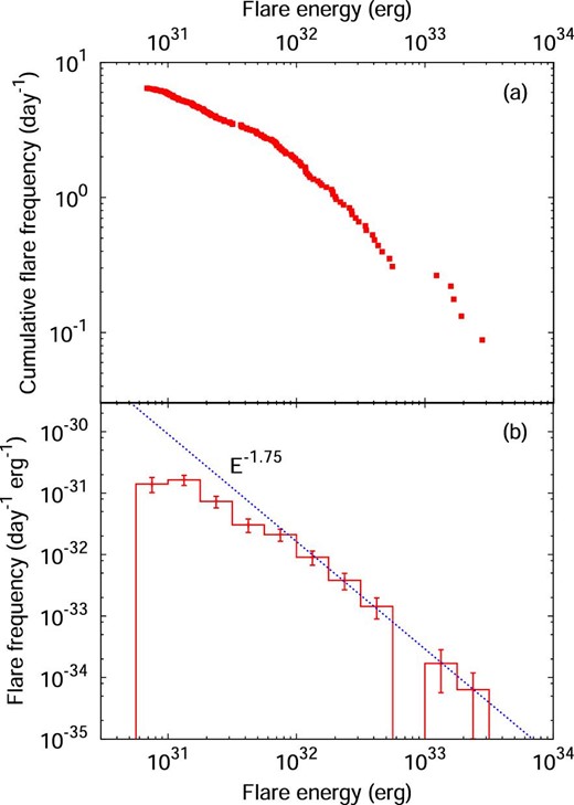
(a) Cumulative flare frequency distribution as a function of flare energy. The horizontal axis is the bolometric energy released by flares. The vertical axis represents the cumulative flare frequency, the number of flares with a flare energy larger than a given value per day. Please note that we cannot detect the flares with occurrence frequency of much less than ∼4.5 × 10⁻² d−1 since the total observation time is ∼22 d. (b) Flare frequency distribution as a function of flare energy. The horizontal axis represents the flare frequency normalized by the bin width. The dotted line represents a power-law fit to the data in the flare energy ranging from 1032 erg to 1034 erg. The power-law index estimated from the fit is −1.75 ± 0.04. (Color online)
3.2 OISTER photometry and spectroscopy
During the OISTER observing campaign, we detected four Hα flares from time-resolved spectroscopy as shown in figures 3, 4, and 5. On 2019 January 16, an Hα flare with a peak timing of 2458500.26 (“flare A”) was detected (figures 3a and 3b). During this flare, Hα and Hβ equivalent widths changed by −2 Å and −7 Å, respectively.7 In addition to the enhancement of the Balmer emission lines, the continuum brightness observed with TESS also increased by 0.3%. We estimated the luminosity of the flare component using the distance to YZ CMi (5.99 pc; Gaia Collaboration 2018), the flux-calibrated quiescent spectra (Kowalski et al. 2013), and g-, RC-, and IC-band magnitudes. The peak luminosity of this flare in the Hα and Hβ lines is 1.2 × 1027 erg s−1 and 0.9 × 1027 erg s−1, respectively (figure 3c). The peak luminosity of this flare in the TESS band is estimated to be 1.5 × 1028 erg s−1 (figure 3d).
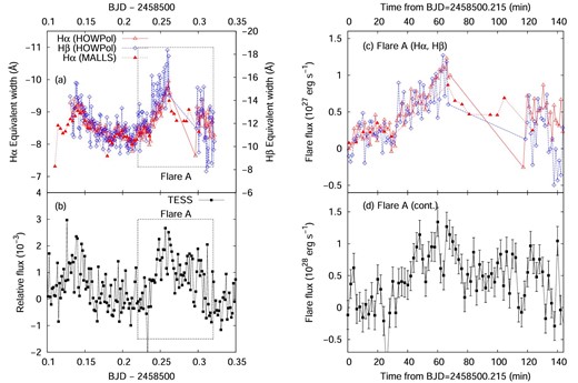
(a) Hα, Hβ light curve of YZ CMi on January 16. The horizontal axis represents the observation time in Barycentric Julian Date (BJD). Left- and right-hand vertical axes represent equivalent widths of the Hα and Hβ lines, respectively (values are negative for emission lines). Open and filled triangles indicate the equivalent width of the Hα line measured from spectra obtained with Kanata/HOWPol and Nayuta/MALLS, respectively. Open diamonds represent the equivalent width of the Hβ line measured from spectra obtained with Kanata/HOWPol. (b) TESS light-curve of YZ CMi during the OISTER observations on January 16. The vertical axis represents the relative flux normalized by the stellar average flux. (c) Enlarged Hα and Hβ light curves of flare A. The horizontal and vertical axis represent the time from BJD 2458500.215 and the flare component’s luminosity. Open triangles and open diamonds indicate the luminosities of the flare component in the Hα and Hβ lines. The flux calibration for the Hα and Hβ lines were performed using the quiescent spectra taken from Kowalski et al. (2013), g- and RC-band magnitudes. (d) Same as panel (c) but for the flare component’s continuum luminosity in the TESS band (6000–10000 Å). (Color online)
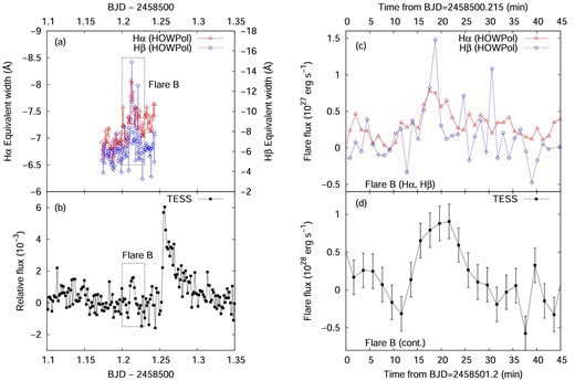
The axes and symbols are plotted as in figure 3. (a) Hα light curve of YZ CMi on January 17. (b) TESS light-curve of YZ CMi during the OISTER observations on January 17. (c) Hα, Hβ light curve of flare B. (d) Same as panel (c) but for the flare component’s continuum luminosity in the TESS band. (Color online)
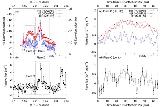
The axes and symbols are plotted as in figure 3. (a) Hα and Hβ light curves of YZ CMi on January 18. (b) TESS light-curve of YZ CMi during the OISTER observations on January 18. (c) Hα and Hβ light curves of flare C. (d) Same as panel (c) but for the flare component’s continuum luminosity in the TESS band. (Color online)
During the short observing run on 2019 January 17, a small and short-duration Hα flare was detected at BJD 2458501.2125 (“flare B”). The equivalent width of the Hβ emission line and continuum flux observed with TESS also increased during this flare (figure 4). The amplitudes of this flare in Hα, Hβ and the TESS band are −1 Å, −4 Å, and 0.2%, respectively. These values correspond to flare peak luminosity of 0.8 × 1027 erg s−1 (Hα), ∼1.2 × 1027 erg s−1 (Hβ), and 0.9 × 1028 erg s−1 (TESS band), respectively.
We detected two Hα flares during the OISTER observation on 2019 January 18. These two flares show different properties: the flare at BJD 2458502.177 (“flare C”) shows slow rise and slow decay, while the double-peaked flare at BJD 2458502.228 (“flare D”) shows rapid rise and rapid decay. For flare C, although the amplitude of the Hα line is comparable to those of flares A and B, we cannot find any clear brightening in the TESS light-curve. The equivalent width of the Hβ line also did not exhibit a clear change during this flare. On the other hand, for flare D, we can see a clear white-light flare with an amplitude of 0.6% in the TESS band, though the flare amplitude of the Hα line is only 50% larger than that of flare C (3 Å). Moreover, the amplitude of flare D in the Hβ line is 11 Å, which is much larger than that of flare C. Flare D was also detected by multi-color photometry observed with MITSuME, as shown in figures 5 b and 5d. The amplitudes of flare D in the g, RC, and IC bands are estimated to be 6.7%, 3.4%, and 0.8%, respectively, using the MITSuME data around the flare peak in the TESS band (from BJD 2458502.227 to 2458502.229). The blackbody fitting to the spectral energy distribution of the flare component around the peak derived from the g-, RC-, and TESS-band data yields an effective temperature of 5900 ± 1000 K, which is comparable to the effective temperature of solar white-light flares (e.g., Watanabe et al. 2013; Kerr & Fletcher 2014; Kleint et al. 2016) and 3000–4000 K lower than the typical effective temperature of white-light flares on M dwarfs (e.g., Hawley & Pettersen 1991; Hawley & Fisher 1992; Hawley et al. 2003; Kowalski et al. 2013). According to Kowalski et al. (2019), the effective temperature of flare components estimated from the optical continuum with a wavelength λ > 4000 Å tends to be low (∼6000 K) for flares exhibiting a large Balmer jump ratio. Kowalski et al. (2013) reported that flares with smaller peak amplitude and longer flare FWHM (full width at half maximum) time tend to show a larger Balmer jump ratio than impulsive flares. As shown in figure 6, flare D is not a impulsive flare because of the small peak amplitude (7.6% in the g′ band) and long flare FWHM time (∼10 min). This morphological property of the light curve for flare D is similar to that for flares showing a low-temperature continuum at λ > 4000 Å.
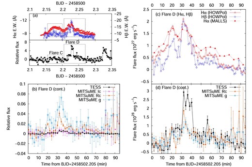
(a) Hα, Hβ and TESS light-curves of YZ CMi on January 18. (b) Light curve of a white-light flare (flare D) on January 18. Filled squares, crosses, asterisks, and open squares represent the brightness change in the TESS band (6000–10000 Å, centered on traditional IC-band; Ricker et al. 2015). IC band (λ0 = 7980 Å, FWHM =1540 Å; Bessell 2005), RC band (λ0 = 6407 Å, FWHM =1580 Å; Bessell 2005), and g band (λ0 = 4770 Å, FWHM =1380 Å; Fukugita et al. 1996) relative to the pre-flare brightness in each band. Each IC-, RC-, and g-band data point and error bar indicate the average value and standard error derived from all data points obtained with MITSuME during each TESS exposure. (c) Hα and Hβ light curve of flare D. (d) Same as panel (a) but for the flare component’s continuum luminosity in the TESS, RC, and g bands. (Color online)
For flare C, the peak flux of the flare component in the Hα line is 1.4 × 1027 erg s−1 (figure 5c), which is comparable to that of flare D (2.1 × 1027 erg s−1; figure 6c). However, the luminosity of the flare component in the TESS-band continuum at the peak timing of flare C is <6 × 1027 erg s−1 (figure 5d). This value is <1/5 of the flare D peak luminosity in the TESS band (figure 6d).
The flare energies released in the optical continuum (TESS band), Hα, and Hβ emission lines for each flare detected by OISTER observations are summarized in table 2. Among these flares, only flare C did not show a white-light flare. For other flares associated with white-light flares, the flare energy released in the TESS-band continuum ranges from 3 × 1030 erg to 3.6 × 1031 erg. The ratio of the flare energy released in the TESS-band continuum to that released in Hα and Hβ lines ranges from ∼5 to ∼20.
List of flares detected by OISTER observations.
| Flare ID | Peak (BJD)* | Peak luminosity (1027 erg s−1) | Energy (1031 erg) | Duration (min) | ||||||
|---|---|---|---|---|---|---|---|---|---|---|
| L TESS † | L bol ‡ | L Hα § | L Hβ § | E TESS † | E bol ‡ | E Hα § | E Hβ § | τflare* | ||
| A | 2458500.260 | 14 | 73 | 1.2 | 0.8 | 2.9 | 15 | 0.25 | 0.3 | 50 |
| B | 2458501.212 | 9 | 48 | 0.8 | ∼1.2 | 0.3 | 1.8 | 0.06 | 0.05 | 15 |
| C | 2458502.177 | <6 | <32 | 1.4 | <0.5 | <0.4 | <2.1 | 0.47 | <0.2 | >70‖ |
| D | 2458502.228 | 29 | 155 | 2.1 | 2.1 | 3.6 | 18 | 0.18 | 0.24 | 35 |
The flare duration and peak time were measured from the Hα light curve obtained with Kanata/HOWPol.
Luminosity and energy emitted in the TESS bandpass (6000–10000 Å).
We assumed that the effective temperature of the flare component, temperature and radius of YZ CMi are 104 K, 3300 K, and 0.3 R⊙.
The flux calibration for the Hα and Hβ lines were performed using the quiescent spectra taken from Kowalski et al. (2013), g- and RC-band magnitudes.
The flare D started before the flare C ended.
4 Discussion
4.1 White-light and non-white-light flares
In this subsection, we focus on two Hα flares (C and D) observed on 2019 January 18. As shown in figure 5, flare C showed a clear increase in the Hα emission line, but no significant flare was observed in the continuum (figure 5). In contrast, flare D showed clear brightening not only in Balmer lines (Hα and Hβ) but also in the continuum (g, RC, IC, and TESS bands). Hα and Hβ light-curves for flare D show two peaks corresponding to two peaks of white-light flare as shown in figure 6. The Hα emission line flux at the peak time of flare C is 1.4 × 1027 erg s−1, which is comparable to that at the peak of flare D (2.1 × 1027 erg s−1). Although the Hα line fluxes at the peaks of flares C and D are roughly the same, the continuum flux in the TESS band at the peak time of flare D (2.9 × 1028 erg s−1) is one order of magnitude greater than that of flare C (<6 × 1027 erg s−1).
The differences between flares C and D are the time-scale of flare and the ratio of the Hα line flux to the continuum flux at the flare peak. The rise time of flare C is much longer than that of that of flare D. In the case of flare C, the equivalent width of Hα emission gradually increased over ∼25 min and decayed over >40 min. The ratio of the Hα line flux to the continuum flux in the TESS band was >0.2 for flare C. In contrast, the rise time of flare D is ∼5 min, which is comparable to that of flare D observed in the continuum light. The peak timings of flare D in Hα, Hβ, and continuum are the same within the time-resolution of observations. The ratio of the Hα line flux to the continuum flux in the TESS band was ∼0.07 for flare D. According to Kowalski et al. (2013), the ratio of the Hα emission flux to the total flux at the flare peak is in the range of 0.0005 to 0.10 for various types of flares on M dwarfs. The ratio of the Hα line flux to the total flux at the peak time of the gradual flares showing slow rise/decay (LHα/Lbol. ∼ 3%–10%) tends to be larger than that of impulsive flares (<1.7%). The difference in the flux ratio of Hα and continuum between the flare C and flare D agree with this tendency.
According to one-dimensional radiative hydrodynamic model calculation of stellar flares on M dwarfs by Namekata et al. (2020b) using the RADYN code (Carlsson & Stein 1997; Allred et al. 2015), the Hα line and continuum intensity increase as the energy deposition rate increases, and the correlation between the intensity of the Hα line (IHα) and that of continuum (Icont.) can be expressed by |$I_{\rm cont.} \propto I_{\rm H \alpha } ^{0.5}$|. This suggests that the fraction of continuum intensity relative to the Hα intensity increases as the continuum intensity increases. In the case of the flare caused by the larger non-thermal electron flux, the ratio of the continuum intensity to the Hα intensity is much larger than that for the flare caused by the smaller non-thermal electron flux. This non-linear correlation between the intensity of the Hα line and that of the continuum suggests that the observed difference in the ratio of the continuum flux to the Hα flux between flare C and flare D can be explained by the difference in the energy deposition rates. This interpretation is also consistent with the fact that the rise time of flare C (small deposition rate) is longer than that of flare D (large deposition rate). The long rise time of flare C suggest that flare C is actually a group of many small flares for which detectable white light emission is not expected. In addition to the continuum flux, the Hβ line flux at the peak time of flare C is also smaller than that at the peak time of flare D. The ratio of Hβ line flux to the Hα line flux (Hβ/Hα) is <0.4 for flare C and ∼1.0 for flare D. Hβ/Hα depends on the electron density, temperature, and optical depth according to Drake and Ulrich (1980). Since the optical depth of the Hβ line is smaller than that of the Hα, the Hβ line flux may behave like the continuum rather than the Hα line flux during the flare. The smaller value of Hβ/Hα for flare C than that for flare D suggests that the electron density of the flare region for flare C is smaller than that for flare D. This may be consistent with the non-thermal electron flux for flare C being smaller than that for flare D.
As mentioned above, although the intensity of the Hα line from the flare region for flare C is expected to be smaller than that for flare D, the peak Hα luminosity of flare C is comparable to that of flare D. This may suggest that the area of flare region for flare C is larger than that for flare D. As we discuss in a later section, the larger area of flare region for flare C would lead to the longer flare duration. Solar non-white-light flares have longer soft X-ray flare durations than white-light flares with a similar Geostationary Operational Environmental Satellite (GOES) X-ray class (e.g., Watanabe et al. 2017) . This tendency is consistent with the differences in the duration and peak continuum flux between flare C and flare D.
4.2 Hα line profile changes during flares C and D
During flare C, the profile of the Hα line showed blue asymmetry (figure 7). As shown in figure 8, the velocity of the blueshifted excess component at the peak time of flare C is −85 ± 3 km s−1. A blueshifted excess component with a line-of-sight velocity ranging from −80 to −100 km s−1 has been seen for 60 min during flare C (figure 9). Around the peak time of flare C, roughly 1/4–1/3 of the Hα emission of the flare component was emitted from the blueshifted excess component. On the other hand, no clear asymmetry in the Hα line profile was observed during flare D (figures 7 and 8).
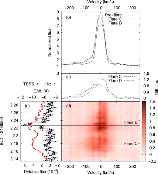
(a) Light curve of YZ CMi during flares C and D. Filled squares (black) and triangles (red) represent continuum flux relative to the average flux observed with TESS and equivalent width of the Hα line observed with Nayuta/MALLS. The vertical axis indicates the time of observation in Barycentric Julian Date (BJD). The lower and upper horizontal axes represent continuum flux relative to the average stellar flux and equivalent width in unit of Å, respectively. (b) Line profile of the Hα emission line. The horizontal and vertical axes represent the Doppler velocity from the Hα line center and flux normalized by the continuum. Solid (black), dashed (green), and, dotted (purple) lines indicate the line profile before flares (BJD 2458502.135), that at the peak timing of flare C (BJD 2458502.177), and that of flare D (BJD 2458502.227). (c) Same as panel (b), but for the line profile changes from the pre-flare to the peak times of flare C and D. (d) Time evolution of the Hα line profile. The horizontal and vertical axes represent the Doppler velocity from the Hα line center and time of observation. The color map represents the line profile changes from the pre-flare profile. (Color online)
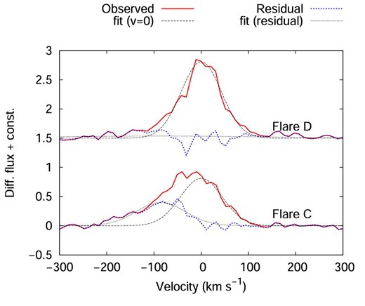
Hα line profile changes from the pre-flare (BJD 2458502.135) to the peak times of flare C (BJD 2458502.177; lower) and D (BJD 2458502.227; upper). Solid lines (red) indicate the observed line profile changes. Dashed lines (black) represent a Gaussian fit assuming the line-of-sight velocity of 0 km s−1 to the red part (>0 km s−1) of the observed line profile changes. Dotted lines (blue) indicate residuals between the observed line profile changes and the Gaussian fits (thin-dashed lines). Black dash–dotted lines represent a Gaussian fit to the residuals (blue dotted lines). The line-of-sight velocity of the residual component (blue enhancement) at the peak time of flare C is −85 ± 3 km s−1. (Color online)
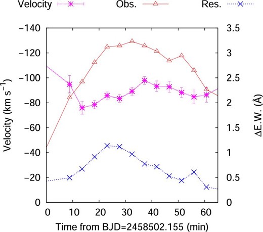
Time variation of the line-of-sight velocity and equivalent width of the blueshifted enhancement during the flare C. Asterisks (magenta) and crosses (blue) indicate the velocity and equivalent width of blueshifted excess component. Open triangles (red) indicate the equivalent width of flare component (change in the equivalent width from the pre-flare state). (Color online)
Since the velocity of the blueshifted component observed during flare C is one order of magnitude larger than the stellar rotation velocity (vsin i ∼6 km s−1; e.g., Houdebine et al. 2016), the observed blue asymmetry cannot be explained by the rotationally modulated emission from the co-rotating prominence (e.g., Collier Cameron & Robinson 1989).
According to Fisher et al. (1985), when the non-thermal electron flux is low, a weak chromospheric evaporation with an upward velocity <30 km s−1 occurs (gentle evaporation). The threshold for the gentle evaporation depends on the energy spectra of non-thermal electron beam (low-energy cutoff and power-law index; Fisher 1989). As discussed above, the weak non-thermal electron flux is suggested from the weak continuum intensity relative to the Hα intensity for flare C. The observed velocity of blue asymmetry during flare C (80–100 km s−1) is a few times larger than the theoretical prediction for solar flares and that of blue asymmetry observed during the gradual phase of solar flares (e.g., Schmieder et al. 1987).
The Doppler velocity of observed blue asymmetry is comparable to that of blue asymmetry observed in chromospheric lines during the initial phase of solar flares, which is proposed to be caused by the cool plasma lifted up by the expanding hot plasma (e.g., Tei et al. 2018; Li et al. 2019). However, the duration of these blue asymmetries (a few min) are roughly two orders of magnitude shorter than that of the blue asymmetry observed during flare C (∼60 min). Honda et al. (2018) reported the similar long-duration Hα flare showing blue asymmetry in the Hα line profile on the M4.5 dwarf EV Lac. The Doppler velocity of blueshifted excess component for this event is ∼100 km s−1 and the blue asymmetry has lasted for >2 hr. Since there were no high-precision photometric data for the Hα flare showing a blue asymmetry reported by Honda et al. (2018), it is unclear whether the typical long-duration Hα flares with blue asymmetry are non-white-light flares like flare C or not.
The observed velocity of the blue asymmetry during flare C is also comparable to the velocity of Hα surges (e.g., Canfield et al. 1996) and that of prominence/filament eruptions (e.g., Gopalswamy et al. 2003) of the Sun. In the case of stellar flares, since we cannot obtain spatial information of the stellar surface, such eruptions and surges may also be possible causes of the blue asymmetry in the Hα line associated with flares. Vida et al. (2016) reported several flares on the M4 dwarf V374 Peg exhibiting blue asymmetry with Doppler velocity ranging from 200 to 400 km s−1. The duration of these blue asymmetries ranges from 10 to 30 min. The similar high-velocity blue asymmetry has been observed during a flare on AT Mic (Gunn et al. 1994). Such high-velocity blue asymmetries during stellar flares are considered to cause stellar CMEs (e.g., Vida et al. 2016). According to Gopalswamy et al. (2003), the average velocity of the core of CMEs (∼350 km s−1) and average CME velocity (∼610 km s−1) are ∼4 and ∼8 times larger than that of the associated prominences (∼80 km s−1), respectively. This indicates that most prominences accelerate as they erupt. If similar acceleration mechanisms would work on YZ CMi, although the velocity of prominence eruption (∼100 km s−1) is smaller than the escape velocity at the stellar surface (∼600 km s−1 for YZ CMi), the upward-moving material would be accelerated to ∼400–800 km s−1. Since this value is larger than the escape velocity at ∼2–3 Rstar (∼350–420 km s−1), even a prominence eruption with a velocity of ∼100 km s−1 could cause a CME. However, it is still unclear whether the prominence eruptions on M dwarfs can cause the stellar CMEs. Crosley and Osten (2018) performed optical and low-frequency radio observations of the M4 dwarf EQ Peg and found no signature of type II bursts, which are believed to be excited by shocks driven by CMEs, during the observed flares. One interpretation for the absence of type II bursts is the magnetic suppression of CMEs in active stars. Numerical studies by Drake et al. (2016) and Alvarado-Gómez et al. (2018) suggest that if the flare region has strong overlying magnetic fields, CMEs will be suppressed. According to Morin et al. (2008), rapidly-rotating mid m (∼ M4) dwarfs such as YZ CMi have mainly axisymmetric large-scale poloidal fields. In the case of YZ CMi, the magnetic energy in dipole mode accounts for ∼70% of the whole magnetic energy, and such large-scale and strong dipole magnetic fields may cause the suppression of CMEs. Another interpretation for the absence of any stellar type II radio burst is that CMEs propagating in the corona/wind of active M dwarfs are “radio-quiet” for ground-based instruments. Mullan and Paudel (2019) proposed that due to the large Alfvén speed in the corona of active M dwarfs, CMEs from these stars could not satisfy the conditions for the generation of type II radio bursts. According to 3D magnetohydrodynamic simulations by Alvarado-Gómez et al. (2020), while CMEs from active M dwarfs can generate shocks in the corona, type II radio burst frequencies are down to the ionospheric cutoff and therefore it is difficult to detect type II radio bursts from active M dwarfs by ground-based instruments.
As shown in figure 9, the velocity of the blueshifted excess component is almost constant (80–100 km s−1) during flare C and the Hα line flux from the blueshifted component decreases as the later part of flare C. In the case of solar CMEs, a prominence forms the core of a CME (e.g., Gopalswamy 2015) and the prominence material can be observed in the Hα line only at early stages. If the prominence on YZ CMi forms the core of a CME and Hα emission from the prominence would disappear as the height of the prominence increases, then the observed blueshifted excess would come from the prominence at the lower layer and the velocity of the blue asymmetry would not change so much during flare C. The intensity of the blueshifted excess may decrease as the mass of the cool material at lower layer decreases. Another interpretation for the persistent blue asymmetry with a constant velocity for ∼1 hr associated with flare C is that it is caused by the ongoing magnetic reconnection and plasma evaporation in the multi-threaded coronal loops (e.g., Warren 2006). If upward velocities of evaporated plasma in each coronal loop would be roughly the same, the velocity of blueshifted excess would also be constant during the flare. However, since our observations are limited (only optical Hα line is used here), it is difficult to distinguish whether the observed blue asymmetry was caused by a prominence eruption, which would cause a stellar CME, or by the chromospheric evaporation in coronal loops. Time-resolved and high-resolution X-ray spectroscopy of stellar flares (e.g., Argiroffi et al. 2019), extreme-UV (EUV) observations for the coronal dimming associated with stellar flares (e.g., Jin et al. 2020), and radio observations for stellar type II bursts (e.g., Crosley & Osten 2018) simultaneously with optical spectroscopy are necessary to investigate the connection between the blue asymmetries in the chromospheric lines and stellar CMEs.
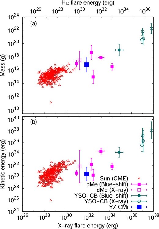
(a) Mass of CMEs/prominences as a function of flare energy. Upper and lower horizontal axes represent the flare energies emitted in the Hα emission line and in X-ray (GOES 1–8 Å band), respectively. The Hα flare energy is converted to the GOES X-ray flare energy using equation (5). Open triangles (red) represent the CME mass of solar events taken from Yashiro and Gopalswamy (2009). The X-ray energy of associated solar flares are derived from the X-ray fluence in the GOES 1–8 Å band. Filled (magenta) squares and filled (cyan green) circles indicate the CME/prominence mass of stellar events on M-dwarfs (dMe), young stellar objects (YSO) and close binary systems (CB) estimated from the blueshifted enhancement of chromospheric lines. Open squares and filled circles also indicate the mass of stellar events on M-dwarfs, young stellar objects, and close binary systems estimated from the X-ray dimming. Mass and X-ray energy for these events are taken from Moschou et al. (2019). The large (blue) filled square indicates the mass of upward-moving material for flare C on YZ CMi. The upper and lower error bars for flare C on YZ CMi represent the mass of upward-moving material estimated in equations (3) and (4). (b) Same as panel (a) but for the kinetic energy of CMEs/prominences as a function of flare energy. (Color online)
4.3 Rotational modulations
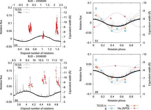
(a) TESS light-curve (solid lines) and Hα equivalent width (open triangles) of YZ CMi around OISTER observation period. The left- and right-hand vertical axes indicate the relative flux in the TESS band and the equivalent width of the Hα emission line. The horizontal axes indicate the number of stellar rotation since BJD 2458498.329. (b) Same as panel (a) but for the light curve around APO observation period. (c) Rotational brightness modulations in the g (open squares), RC (asterisks), and TESS (black dots; large flares were excluded) bands observed during the TESS cycle 7 and the rotational modulation of the Hα equivalent width (red triangles) obtained by OISTER observations; g-band, RC-band, and Hα data indicate the average value during each observation run except for the data during flares. The rotation phase was calculated from equation (6). Blue dotted, orange dashed, and red dash–dotted lines indicate sinusoidal fits to g-band, RC-band, and Hα line data. (d) Same as panel (c) but for the rotational modulations of the equivalent width of the Hα emission line obtained by APO observations. (Color online)
During the OISTER observations, the intensity of the Hα line shows the anti-correlated rotational modulation with that in the continuum light (figure 11a). Since the amplitude of rotational modulation in Hα (11%) is slightly larger than that of the rotational modulation in the RC band (7.4%), the rotational modulation in the Hα line cannot be produced only by that in the RC band if we assume that the Hα line flux is constant over the rotation phase and only the continuum intensity changes due to the rotation. On the other hand, the rotational modulation in the Hα line cannot be seen in the data obtained during the APO observations. The Hα line intensity is almost constant over the rotation phase (figure 11b). These results suggest that bright regions in the Hα line are concentrated at the darker side in the continuum (rotation phase of 0.5) during the OISTER observation period, and the Hα line intensity at the brighter side in the continuum (rotation phase of 0) has increased before or during the APO observations. As shown in figure 1b and 1c, the number of flares during the OISTER observations is smaller than that during the APO observations, and large flares occurred just before and during the APO observations at the rotation phase of ∼0.7–0.8. This suggests that the Hα intensity of the existing active region, which can be seen around the rotation phase of ∼0.7–0.8, has increased due to a new flux emergence that makes the active region more flare-productive, or a new flare-productive active region has appeared at the longitude corresponds to the rotation phase of ∼0.7–0.8. Since such active regions would be bright in Hα line, they can change the light curve shape of rotational modulation in Hα line. Since the rotational modulations in the continuum are almost the same between these two observations while the rotational modulations in the Hα line are different, the sizes and locations of starspots may not change, or the size of starspots associated with the new active region may not be so large. According to Vida et al. (2016), anti-correlated modulations in the Hα line and in the optical continuum were reported in an active M dwarf V374 Peg during the observations in 2009. However, this anti-correlation is unclear for the data obtained in 2005 and 2006. These differences in rotational modulations between the data in 2005–2006 and in 2009 may also be explained by the difference in the surface distribution of active regions.
Figure 12 shows (a) rotational brightness variation, (b) flare frequency as a function of rotation phase, and (c) bolometric energy of each flare as a function of rotation phase. There is no clear correlation between the rotation phase and flare activities such as flare frequency or the energy of the largest flare in each phase bin. Similar results have been reported by Hawley et al. (2014) and Silverberg et al. (2016) in the active M dwarf GJ 1243, and by Doyle, Ramsay, and Doyle (2020) in active solar-type stars. They found that the flare frequency and flare energy do not depend on rotation phase. Hawley et al. (2014) and Davenport, Hebb, and Hawley (2015) proposed two possible interpretations for this property: (1) A large fraction of the polar region is covered by starspots and flares come from the large starspots near the pole. The rotational modulation of stellar brightness in the optical continuum is mainly caused by the rotational change in the apparent area of starspots near the pole if the location of the polar spot is slightly shifted from the rotation axis or if the polar spot is not completely axisymmetric. Since the starspots near the pole can always be seen by the observer, the flare frequency does not depend on the rotation phase. (2) Most of the flares come from many relatively small active regions which contain large amounts of stellar magnetic flux (Reiners & Basri 2009), while the polar spot is associated with the global dipolar magnetic field (Morin et al. 2008). Since these many small active regions are distributed across longitude (e.g., Namekata et al. 2020a; Takasao et al. 2020), they cannot produce significant brightness modulation (e.g., Schrijver 2020) compared to that from the large polar spot and the flare frequency would not depend on the rotation phase.
A strong correlation between the core emission of Ca H and K lines and the magnetic field strength (e.g., Schrijver et al. 1989; Notsu et al. 2015) suggests that the origin of chromospheric emission is magnetic. As mentioned above, although the rotational modulations in the Hα line are different between two observations, the rotational modulations in the continuum are almost the same. The possible explanations for the observed changes in rotational modulations based on the possible interpretations for the rotational modulations of flare frequency are as follows: During the low-activity period, both rotational modulations in the optical continuum and in the Hα line are mainly produced by the polar spot and surrounding active regions. Since both the apparent area of a polar spot and that of the surrounding active regions change as the star rotates, rotational modulations in the continuum and in the Hα line would be anti-correlated. In the case of a high-activity period, although the rotational modulation in the optical continuum is also produced by the polar spot, most of the Hα line emission comes from many relatively small active regions which are distributed across longitude. Therefore the Hα line intensity does not depend on the rotation phase during the high-activity phase. Since the chromospheric emission is thought to be correlated with the flare activity, these results on the rotational modulation of the Hα line intensity suggest that the constant flare frequency over the rotation phase on active M dwarfs can be explained if most of the flares occur on many smaller active regions across the entire stellar longitude.
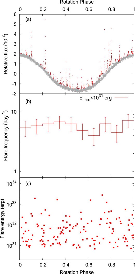
(a) Phase-folded light curve of rotational brightness variations observed with TESS. The rotation phase was calculated from equation (6). Red dots indicate the data points which are identified as flares. (b) Frequency of flares with the bolometric energy larger than 1031 erg as a function of rotation phase. Error bars indicate the square-root of the number of flares in each phase bin. (c) Bolometric energy of each flare as a function of rotation phase. (Color online)
4.4 Flare duration vs. flare energy
Figure 13 shows the scatter plot of the duration (e-folding time) of flares on YZ CMi observed with TESS as a function of flare energy. We estimated the e-folding time by the exponential fit to the data for each flare from the flare peak time (t = tpeak) to t = tpeak + 2(t1/e − tpeak), where t1/e is the time that the flare flux decays to 1/e of the peak flux. We can see a positive correlation between the flare duration (τflare) and the bolometric flare energy (Eflare). The duration of flares increases with energy as |$\tau _{\rm flare} \propto E_{\rm flare}^{0.21\pm 0.04}$|. The power-law slope of the correlation between the flare duration and energy for flares on YZ CMi is smaller than that for flares on G-dwarfs observed with Kepler (Maehara et al. 2015) and with TESS (Tu et al. 2020).
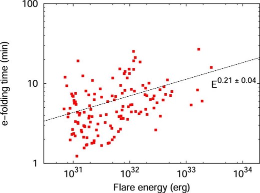
Scatter plot of flare duration (vertical axis) as a function of the bolometric flare energy (horizontal axis). We used e-folding time from the flare peak time as the duration of flares. The bolometric flare energy was estimated from the TESS light-curve under the assumption that the spectral energy distribution of the flare component can be represented by the blackbody radiation with the temperature of 104 K. (Color online)
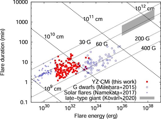
Comparison of τ–E relations for solar white-light flares (blue crosses; Namekata et al. 2017), stellar flares on an M dwarf YZ CMi (red filled squares; this work), superflares on solar-type stars (blue open circles; Maehara et al. 2015), and superflares on a late-type giant KIC 2852961 (gray area; Kővári et al. 2020). Dashed lines indicate τ–E relation based on equation (11) for B = 30, 60, 200, and 400 G. Dotted lines represent another τ–E relation based on equation (12) for L = 109, 1010, 1011, and 1012 cm. (Color online)
4.5 Flare duration statistics
According to Veronig et al. (2002), the frequency distribution of solar flares as a function of the flare duration can be represented by a power-law function with a power-law index of −2.9. Similar plots of the frequency distribution as a function of the flare duration (e-folding time) for the flares on YZ CMi are shown in figure 15. We found that the frequency distribution of flares on YZ CMi as a function of the flare duration can also be well represented by a power-law function with a power-law index of −2.8 ± 0.1. This value is comparable to the power-law index for the frequency distribution of solar flares. This similarity in flare frequency distribution as a function of flare duration may come from the similarity in the flare frequency distribution as a function of flare energy and that in the duration–energy correlations for solar flares observed in soft X-rays and for stellar flares observed in optical. The flare frequency distribution as a function of energy (flare fluence) can be well represented by a power-law function (dN/dE ∝ Eα) with a power-law index of α = −2.03 for solar soft X-ray flares (Veronig et al. 2002). In the case of optical flares on YZ CMi, the flare frequency distribution as a function of the bolometric energy of flares can also be represented by a power-law function with a power-law index of −1.75. Moreover, both the duration–energy (flare fluence) correlation (|$\tau _{\rm flare} \propto E_{\rm flare} ^{\beta }$|) for solar soft X-ray flares and that for optical flares on YZ CMi show a similar power-law slope (∼1/3 for solar flares: Veronig et al. 2002; ∼0.2 for YZ CMi: this work). These similarities between the statistical properties of solar flares and those of stellar flares suggest that the energy-release mechanisms are the same for solar and stellar flares.
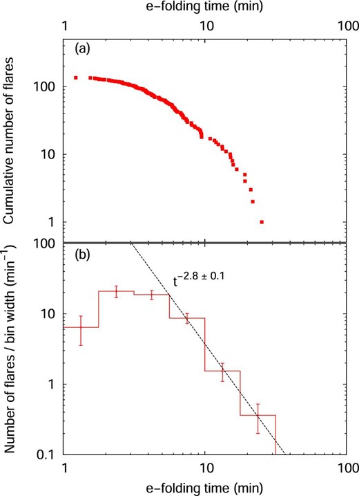
Number of flares as a function of flare duration. The vertical and horizontal axis indicate the number of flares in each bin and e-folding time of flares. (Color online)
5 Summary and conclusions
We carried out time-resolved photometry and spectroscopy of the M-type flare star YZ CMi during the TESS observation window. We detected four Hα flares from our spectroscopic and photometric observations, and one of them exhibited no clear brightening in the continuum. The key findings from our observations are as follows:
The Hα flares with brightening in the continuum tend to have shorter flare duration and larger Hβ emission line flux than the non-white-light flare.
During the non-white-light flare, the blue asymmetry in the Hα emission line was observed for ∼60 min. The line-of-sight velocity of the blue asymmetry was in the range from −80 to −100 km s−1.
If we assume the blue asymmetry in the Hα line was caused by a prominence eruption, the mass and kinetic energy of erupted material are estimated to be 1016–1018 g and 1029.5–1031.5 erg, respectively. Although these values are comparable to those expected from the empirical relations between flare X-ray energy and mass/kinetic energy for stellar events, the estimated kinetic energy is two orders of magnitude smaller than that expected from the empirical relation for CMEs on our Sun. This could be understood by the difference between the velocity of prominence eruption and that of CMEs. More simultaneous optical and X-ray/EUV/radio observations are necessary to fully understand stellar CMEs.
The TESS light-curve shows rotational modulations with a period of 2.7737 ± 0.0014 d and full-amplitude of 3.6%. The rotational modulations can also be seen in g- and RC-band data. The amplitude of the rotational modulations increases as the wavelength decreases (9.8% in the g band and 7.4% in the RC band). These rotational modulations suggest that 10%–20% of the surface of YZ CMi would be covered by starspots.
The rotational modulation can also be seen in the equivalent width of the Hα line during the OISTER observation. The Hα line modulation was anti-correlated with rotational modulations in the continuum. However, the equivalent width of the Hα line was almost constant during the APO observation. The TESS light-curve suggests that the difference in rotational modulations in the Hα line between these observations may be caused by the difference in the flare activity during each observation run.
The flare frequency and the largest flare energy during the TESS observation period were roughly constant over the rotation phase.
The duration of flares (τ) observed with TESS shows a positive correlation with the flare energy. The flare duration distribution shows the power-law distribution (dN/dτ∝τα) with the power-law index of α = −2.8 ± 0.1, which is consistent with the power-law index of the flare duration distribution for solar flares.
Supplementary data
Data set of 145 white-light flares identified in TESS (table_S1.csv).
Acknowledgements
This work was supported by the Optical and Near-infrared Astronomy Inter-University Cooperation Program and the Grants-in-Aid of the Ministry of Education. This work was also supported by MEXT/JSPS KAKENHI Grant Numbers JP17K05400, JP20K04032 (H.M.), JP18J20048 (K.N.), and JP17K14253 (M.Y.). Y.N. was supported by JSPS Overseas Research Fellowship Program. Y.N. also acknowledges the International Space Science Institute and the supported International Team 464: “The Role Of Solar And Stellar Energetic Particles On (Exo)Planetary Habitability (ETERNAL, http://www.issibern.ch/teams/exoeternal/)”. This paper includes data collected with the TESS mission, obtained from the MAST data archive at the Space Telescope Science Institute (STScI). Funding for the TESS mission is provided by the NASA Explorer Program. STScI is operated by the Association of Universities for Research in Astronomy, Inc., under NASA contract NAS 5-26555. In this study, we used the observation data obtained with the Apache Point Observatory (APO) 3.5 m telescope, which is owned and operated by the Astrophysical Research Consortium. We used APO observation time allocated to the University of Washington, and appreciate Suzanne Hawley for helping to plan the observation. We are grateful to APO 3.5m Observing Specialists and other staff members of Apache Point Observatory for their contributions in carrying out our observations. We are grateful to Mr. Isaiah Tristan (University of Colorado Boulder) for valuable suggestions to improve the manuscript. We thank Dr. Jun Takahashi (Nishi-Harima Astronomical Observatory, Center for Astronomy, University of Hyogo) for his support for our observation using Nayuta Telescope. We also thank Prof. Jeffrey Linsky for useful comments and suggestions that contributed to improve the manuscript.
Footnotes
IRAF is distributed by the National Optical Astronomy Observatories, which are operated by the Association of Universities for Research in Astronomy, Inc., under cooperate agreement with the National Science Foundation.
PyRAF is part of the stscipython package of astronomical data analysis tools and is a product of the Science Software Branch at the Space Telescope Science Institute.
The equivalent width of a spectral line is defined as an area of the line on a plot of the continuum-normalized intensity as a function of wavelength. In this paper, since a negative value of the equivalent width indicates line emission, a decrease (negative change) of equivalent width indicates an increase of emission line flux.
References
