


Abstract
We analyzed the data of Stokes I, Q, and U in the C and X bands and investigated the large-scale magnetic field structure of NGC 3627. The polarization intensity and angle in each band were derived using Stokes Q and U maps. The rotation measure was calculated using polarization angle maps. Moreover, the magnetic field strength was calculated by assuming energy equipartition with cosmic ray electrons. The structure of the magnetic field was well aligned with the spiral arms, which were consistent with those in the former studies. We applied the magnetic vector reconstruction method to NGC 3627 to derive a magnetic vector map, which showed that the northern and southern disks were dominant with inward and outward magnetic vectors, respectively. Furthermore, we considered the large-scale structure of the magnetic field in NGC 3627 and observed that the structure is bi-symmetric spiral in nature, and that the number of magnetic field modes is mB = 1 in the outer region of galaxy. In addition, NGC 3627 has a mode of two spiral arms that were clearly visible in an optical image. The ratio of the mode of the spiral arms to that of the magnetic field is 2 : 1. In terms of NGC 3627, the large-scale magnetic field may be generated via the parametric resonance induced by the gravitational potential of the spiral arms.
1 Introduction
Although we know that magnetic fields are ubiquitous in the universe, from the stellar scale to the large-scale structure, our understanding of the role of the magnetic field is not yet complete (Beck 2016). Large-scale magnetic fields of nearby galaxies are aligned well with the galactic spiral arms, which can be traced well in optical or infrared images (Beck 1982, 2015; Han et al. 1999). We do not understand whether the origin of the regular magnetic field is the amplified primordial magnetic field or that generated by a mean-field dynamo (Han 2017).
The structure of magnetic fields is studied on the basis of observations of synchrotron radiation. Notably, this radiation has a polarized component, and the orientation of the magnetic field can be derived by rotating the polarization angle by 90°. The sign of the rotation measure (RM) indicates the direction of the line-of-sight component of the magnetic field. Positive or negative RM indicates that the magnetic field is directed toward us or away from us, respectively. The absolute value of RM is represented by the product of the number density of thermal electrons and the magnetic field strength along the line of sight. There is a method of examining the magnetic field structure of nearby galaxies by using the azimuthal variation in RM (Sofue et al. 1985). Accordingly, the regular magnetic field structure of some nearby galaxies has been studied using this method (Beck & Wielebinski 2013). Magnetic field structure is classified as an axis-symmetric spiral (ASS), which has a pitch angle and either an outward or inward magnetic component, or a bi-symmetric spiral (BSS), which has a pitch angle and both outward and inward magnetic components. Some studies showed magnetic field vectors without the 180° ambiguity by comparing multiple-frequency data with theoretical models (Fletcher et al. 2004; Beck et al. 2005). The M51 disk and halo structures were studied by the same method (Fletcher et al. 2011). Recently, a magnetic vector reconstruction method was developed by Nakanishi, Kurahara, and Anraku (2019). Notably, Kurahara and Nakanishi (2019) applied the method to NGC 6946 to study its large-scale magnetic field.
In this study we focus on NGC 3627, which is located at [RA (J2000.0), Dec (J2000.0)] = (|${11{^h}20{^m}15{^{\s}_{.}}0}$|, +12°59′29′′) and is classified as morphological type SAB(s)b (de Vaucouleurs et al. 1991). In addition, it is at a distance of 11.1 Mpc (Hoyt et al. 2019), at which an angular size of 1″ is equivalent to a physical scale of 54 pc. The position angle and inclination of NGC 3627 are 176° and 52°, respectively (Kuno et al. 2007). These basic pieces of information regarding NGC 3627 are listed in table 1. NGC 3627 is one of the Leo Triplet group of galaxies (Arp 1966). Its stellar disk has been reported to have two strong spiral arms (Martínez-García & Puerari 2014).
Basic parameters of NGC 3627.
Basic parameters of NGC 3627.
The polarized synchrotron emission of this source has been used by Soida et al. (1999) to study its magnetic field; they reported the total intensity and polarization maps of NGC 3627 on the basis of X-band observation using the Effelsberg 100 m telescope. The polarization intensity was smoothly distributed in the galactic disk, with a strong polarization component in the dust lane of the western arm and a weak component between the spiral arms in the northeast. Additionally, on the basis of C- and X-band observations, Soida et al. (2001) reported that the direction of the magnetic field was well aligned with the arm on the western side of the disk.
In this paper we report on the magnetic field structure of NGC 3627; the structure was obtained by applying the magnetic vector reconstruction method to NGC 3627. In section 2 we summarize the data used in this study, and in section 3 we describe the magnetic vector reconstruction method. Section 4 shows the results, which include the magnetic field strength and magnetic vector map. In section 5 we discuss the results obtained. Finally, in section 6, we provide a summary.
2 Data
2.1 Data reduction
The data used in this study were published by Soida et al. (2001) and obtained from observations in the C band (4.85 GHz) and X band (8.46 GHz). They consist of a combination of single-dish and interferometry data, obtained with the Effelsberg radio telescope and very large array (VLA), respectively. Observational information, such as the frequency, size of the synthesized beam, and root mean square (rms) noise, are summarized in table 2.
Observational parameters.
| C | X | |
|---|---|---|
| Frequency | 4.85 GHz | 8.46 GHz |
| Beam size | |${13{^{\prime \prime }_{.}}5}$| × |${13{^{\prime \prime }_{.}}5}$| | |${11{^{\prime \prime }_{.}}0}$| × |${11{^{\prime \prime }_{.}}0}$| |
| Stokes I rms | 66 |$\rm { \mu Jy\, beam^{-1}}$| | 27 |$\rm { \mu Jy\, beam^{-1}}$| |
| Stokes Q rms | 11 |$\rm { \mu Jy\, beam^{-1}}$| | 6 |$\rm { \mu Jy\, beam^{-1}}$| |
| Stokes U rms | 10 |$\rm { \mu Jy\, beam^{-1}}$| | 6 |$\rm { \mu Jy\ beam^{-1}}$| |
Data analysis was performed using the AIPS (Astronomical Image Processing System) software. We calculated the polarization intensity and polarization angle using the AIPS task COMB. Using the Stokes parameter, the polarization intensity and angle were calculated to be |$P_{\rm POL} = \sqrt{Q^2 + U^2}$| and |$\chi = \frac{1}{2}{\rm arctan} ( U / Q )$|, respectively. The polarization intensity was corrected by subtracting the positive bias using the task POLCO. The primary beam was also corrected using the task PBCORL. The noise level σ of each Stokes parameter was the variance of the emission-free region and measured using TVBOX and IMSTAT, both of which are parts of AIPS. The measured noise levels are summarized in table 2. The detection limit was defined as three times the noise level, i.e., 3 σ.
2.2 Radio images
We derived the total and polarized intensities in the C and X bands. Figure 1 depicts the contours of the total intensities and orientations of the B field (90° rotation of the E field) overlaid on a black-and-white image from DSS2 B (McLean et al. 2000). The observed B field is plotted only in pixels in which the polarized intensities were detected with higher signal-to-noise (S/N) ratio than the detection limit in Stokes Q and U [>3(σQ + σU)/2].

Maps of the total intensity (contour) and orientation of the magnetic field (white bars) of the C (left) and X (right) bands of NGC 3627. The background is a black-and-white image of DSS2 B (McLean et al. 2000). The orientation of the magnetic field was obtained by rotating the observed polarization plane by 90°. The white lines are plotted every 7″ in the C band and 5″ in the X band, by considering the spatial resolution. The beam is drawn at the lower left of each map, the beam sizes being |${13{^{\prime \prime }_{.}}5}$| and |${11{^{\prime \prime }_{.}}0}$|, respectively. The contour intervals are (3, 6, 12, 24, 48, 96) × 66 μJy beam−1, (3, 6, 12, 24, 48, 96) × 27 μJy beam−1.
The total intensity is brightest in the boundary region between the southern bar and spiral arm, at 12.99 and 9.19 mJy beam−1 in the C and X bands, respectively. This region is also bright in CO and H i lines (Kuno et al. 2007; Walter et al. 2008). The polarized intensity is brightest in the galactic central region in the X band and in the southwestern spiral arm in the C band.
2.3 Rotation measure
A histogram of the calculated RM is depicted in figure 2. We fitted the histogram of RM with a Gaussian function by using the nonlinear least squares method, which is based on the Levenberg–Marquardt method. The peak value of the fitted Gaussian was 27.9 at +56.5 rad m−2, and the dispersion was 48.3 rad m−2, which is consistent with the value for galaxies (Beck 2016). We attributed +56.5 rad m−2 to the foreground.
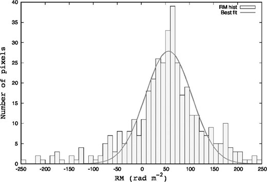
RM histogram of NGC 3627. The horizontal axis represents RM rad m−2 and the vertical axis represents the number of pixels. The Gaussian that was the best fit within the absolute value of RM within 250 rad m−2 was drawn using a solid line. The horizontal axis is drawn with a resolution of 10 rad m−2.
In figure 3 we depict an RM map of NGC 3627 in which the foreground RM of +56.5 rad m−2 was subtracted. The color range indicates the RM value. The contour levels are −150.0, −131.25, −112.5, −93.75, −75.0, −56.25, −37.5, −18.75, 0.0, 18.75, 37.5, 56.25, 75.0, 93.75, 112.5, 131.25, and 150.0 rad m−2. This distribution is consistent with that reported by Soida et al. (2001).

RM map of NGC 3627 at angular resolution |${13{^{\prime \prime }_{.}}5}$|. RM +56.5 rad m−2 in the foreground was removed. The pixels that had an absolute value of RM greater than 200 were masked as unrealistic. (Color online)
3 Magnetic vector reconstruction method
We used the magnetic vector reconstruction method, which is described in Nakanishi, Kurahara, and Anraku (2019). The method can be used to determine the directions of magnetic vectors without the 180° ambiguity by using observational data. The directions of magnetic vectors are derived from the multifrequency radio data of synchrotron polarization after determining the orientation of a disk on the basis of the shape of spiral arms and the velocity field. The advantage of this method is that the magnetic field vector of a galaxy can be determined using only simple assumptions and observational data. More details are described below.
First, we must examine the direction of galactic rotation. Because spiral galaxies generally have trailing spiral arms (Iye et al. 2019), NGC 3627 rotates counter-clockwise in the sky plane, as depicted in figure 4a. Next, we used the velocity map of H i data to determine the geometrical orientation. We observed that the east side was the near side, as the northern and southern parts were blue- and redshifted, respectively, as depicted in figure 4b. The orientations of the magnetic field at individual pixels are given by the synchrotron polarization angle of a higher-frequency band, with 180° ambiguity, as depicted in figure 4c. This ambiguity was solved by checking the sign of RM, as depicted in figure 4d. If the RM of a pixel is positive, the magnetic field component along the line of sight of the pixel is directed toward us from the source, and vice versa. Because the eastern side of the disk is close to us, as previously mentioned, the vector is directed southeastward, as depicted in figure 4d. Therefore, the directions of all the magnetic vectors can be determined point by point, as depicted in figure 4e, where the inward and outward vectors are plotted in red and blue, respectively. Finally, we can derive a magnetic vector map, as depicted in figure 4f.
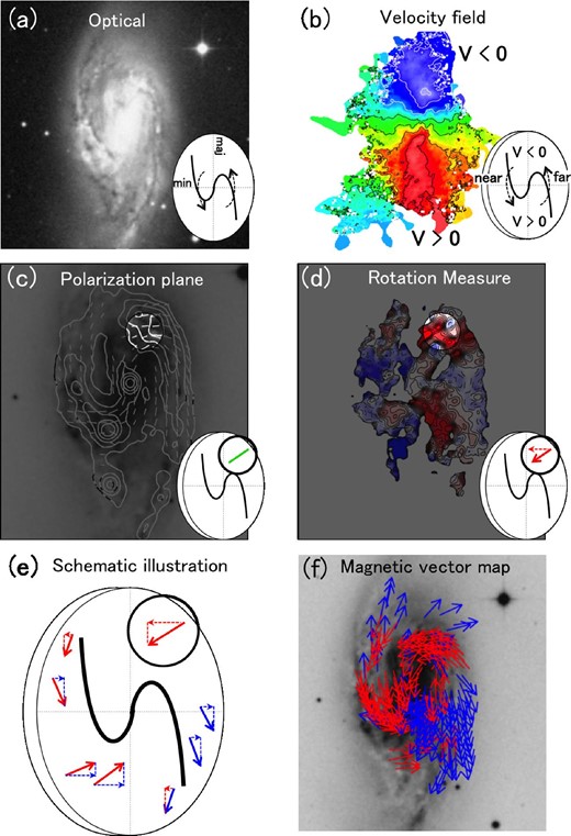
Steps in the magnetic field vector reconstruction method (Nakanishi et al. 2019). (a) Determine the direction of rotation of the galaxy on the basis of an optical image after assuming a trailing spiral. (b) Determine the near side of the galaxy by combining the map of the velocity field and the direction of rotation. (c) Determine the direction of the magnetic field perpendicular to the line of sight from the polarization plane of the synchrotron (with an ambiguity of 180° along the line of sight). (d) Solve the 180° ambiguity along the line of sight using the sign of RM. (e) Determine the direction of all the magnetic vectors. (f) A magnetic vector map of NGC 3627 can be derived. (Color online)
Notably, in our analysis we ignored the southeastern region, where the H i velocity field significantly deviates from its galactic rotation. This region is not detected in synchrotron emission.
4 Magnetic field of NGC 3627
4.1 Strength of magnetic field
The strength of the ordered component can be obtained by using the equation Bord = Btot/(1 + q2), where q is the ratio of the turbulent to ordered components. The ratio q is given by |$q \simeq \sqrt{2.1\ p_0/p}$|, where p is the observed polarization degree and p0 is the intrinsic polarization degree. The polarization degree p was calculated using Stokes I and PPOL,corrected values (p = PPOL,corrected/I). PPOL,corrected is the corrected polarization intensity of positive bias. The intrinsic polarization degree p0 is determined using the spectral index as p0 = (3 − 3α)/(5 − 3α), as described in Beck and Krause (2005). We adopted α = 0.9, K0 = 100, L = 6.2 × 1021 cm, Ep = 1.5 × 10⁻³ erg, c2 = 3.9 × 10⁻²⁴ erg G−1 sterad−1, and c4 = 0.622 to estimate the magnetic field strength, by following former works (Soida et al. 2001; Beck & Krause 2005).
The radial distribution of the magnetic field strength and its equivalent energy density are depicted in figure 5. The averaged magnetic field strength over the galaxy is Btot = 18.8 ± 4.2 μG for the total field, and Bord = 6.1 ± 2.0 μG for the ordered field. Although the total field is highest at the galactic center and decreases with radius, it is roughly constant in the range r = 1.5–5.5 kpc. The ordered field is almost constant for all radii. The error bars are the standard deviation of each data within the corresponding radius range.
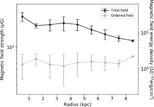
Radial distribution of the magnetic field strength. The horizontal axis represents the radius from the galactic center, in kpc, and the left and right sides of the vertical axis represent the magnetic field strength in μG and the energy density equivalent to a magnetic field strength of 10−12 erg cm−3. The black solid line indicates the total magnetic field strength, and the gray dashed line indicates the ordered field.
where νmin and νmax denote the ranges of the spectrum for synchrotron radiation.
In Soida et al. (2001), the cutoff value of the lower electron energy was 300 MeV. Therefore, we adapted νmin = 500 MHz, which was converted from 300 MeV [e.g., equation (2) of Reynolds and Keohane (1999)], and νmax = 10 GHz. Furthermore, when we calculated Bord,class using the classical method, the polarization intensity was used directly as Iν instead of dividing it by q. From the abovementioned results, it is considered that the difference between our results and those of Soida et al. (2001) can be attributed to the difference between the methods used.
4.2 Magnetic field vector map
We derived a magnetic field vector map using the magnetic vector reconstruction method, as explained in section 3. The left panel of figure 6 shows a magnetic field vector map of NGC 3627. The magnetic field vectors were plotted only at points that satisfied the following four criteria: (1) Stokes I and PPOL higher than 3 σI and 3(σQ + σU)/2 in the C and X bands, respectively; (2) RM higher than the detection limit (σRM), which was calculated on the basis of error propagation using the expression |$\sigma _{\rm RM} = \sqrt{[\delta \chi (\lambda _1)^2 -\delta \chi (\lambda _2)^2]/ ({\lambda _1^2}-{\lambda _2^2})^2}$|; (3) absolute value of RM within 200 rad m−2; and (4) the difference in polarization angle in each band is larger than the sum of the polarization angle errors. We used the polarization angle in the X band as the orientation of the magnetic vector. We neglected the Faraday rotation due to the intervening media between the source and our location, as the typical RM dispersion was 48.3 rad m−2, which corresponds to a few degrees of rotation in the X band.
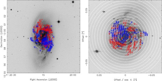
(Left) Magnetic field vector map of NGC 3627 in the sky plane. The effective angular resolution is |${13{^{\prime \prime }_{.}}5}$|. The background is the same as in figure 1. The red and blue arrows show inward and outward magnetic vectors, respectively. The vectors are plotted every 7″. (Right) The face-on view of the magnetic field vector map, made by rotating counter-clockwise by the position angle and extending in the minor-axis direction by 1/cos i. The white circles are drawn at intervals of 1.0 kpc from the center of the galaxy. (Color online)
In the right panel of figure 6, we show a face-on view of the magnetic field vector map. It was made by rotating the left panel counter-clockwise by the position angle of 176° to align the major axis with the vertical axis, and horizontally enlarging it by a factor of 1/cos i. We observed that NGC 3627 has both inward (red) and outward (blue) magnetic field vectors, suggesting that the structure of the magnetic vector is not ASS. In the left panel of figure 6, we show that the vectors in the northeastern and southwestern regions are inward and outward, respectively. Therefore, the BSS mode seems dominant in this galaxy, as discussed in the following section.
5 Large-scale magnetic vector structure
5.1 Definitions of pitch angle, vector angle, and inward/outward sign
As shown in the upper-right panel of figure 7, the angle of the magnetic vector is defined as the angle between the tangent of the circle and the magnetic vector. For instance, a pitch angle of 0° corresponds to a vector angle of 0° or −180°. Azimuth is defined counter-clockwise from the major axis of the galaxy, as shown in the upper-left panel of figure 7. The bottom-left and bottom-right panels show the vector map within a ring of 3.0–4.0 kpc, and the corresponding azimuthal profile of the magnetic vector angle, respectively.
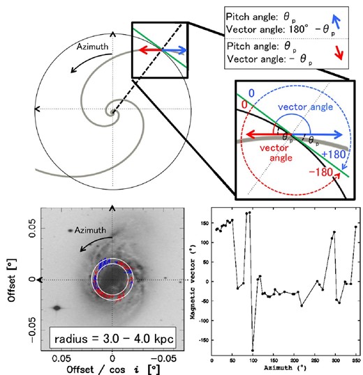
Schematic and definition of galactic azimuth and magnetic field vector angle. The bottom-left and bottom-right panels show a magnetic vector map within a ring of 3.0–4.0 kpc and azimuthal profiles of magnetic vectors, respectively. (Color online)
5.2 Mode of magnetic field based on reversal
We studied the modes of the magnetic field by focusing on the reversals of the magnetic vector. It can be seen from figure 6 that NGC 3627 has both inward and outward magnetic vectors. The panels of the first and third columns of figure 6 show magnetic vector maps within individual rings at radial intervals of 18″ (=1.0 kpc), and panels of the second and fourth columns show whether the magnetic vectors were directed inward or outward at the azimuthal resolution of |${13{^{\prime \prime }_{.}}5}$| (=beam size). Inward and outward vectors in figure 8 were defined as −1 and +1, respectively. We considered the most frequent value of three successive data points, which was obtained by |$most\_frequent\_value( s_{j-1}, s_{j}, s_{j+1})$| with the sign of the jth data point defined as sj. The red and blue dots of the azimuthal profiles indicate inward and outward vectors, respectively.
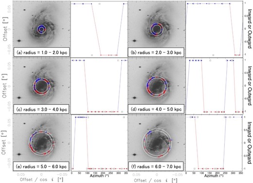
Columns 1 and 3: Face-on views of the magnetic vector map of radius ranges of 1.0–7.0 kpc. Columns 2 and 4: Azimuthal profiles of magnetic vector angle. (Color online)
If the magnetic field has mode mB, 2mB reversals can be found azimuthally. Therefore, we studied the mode of the magnetic field by counting the number of magnetic field reversals. We found mB = 2 in figure 8d, and mB = 1 in the others. Therefore, we found that the magnetic mode of mB = 1 was dominant in NGC 3627. The radius with mB = 2 corresponds to the bar-end region at a radius in the range of 4.0 to 5.0 kpc (Watanabe et al. 2011; Zhang & Buta 2015). This is consistent with the result of Beck et al. (2005), in which regular magnetic fields change the sign in the bar-end region. For rings of radius in the range of 0.0 to 1.0 kpc and >8.0 kpc, the magnetic mode was not included because there were few data points (<6 points). These results for mB are consistent with those reported by Soida et al. (2001), who found mixed magnetic field modes.
The mode of mB = 1 in the outer region (r > 5.0 kpc) corresponds to the BSS structure. NGC 3627 has two spiral arms, which means that the mode of the spiral arms is mD = 2 (Martínez-García & Puerari 2014). Therefore, we observed that the relationship between the modes of the spiral arms and the magnetic field was mB = mD/2 in NGC 3627. This is in good agreement with the results of analytical galactic dynamo models reported by Chiba and Tosa (1990). They indicated that two-armed spiral galaxies, that is, mD = 2, can have the BSS structure due to swing excitation. The growth of the magnetic field in this dynamo is described as a parametric resonance driven by the velocity profile around the density wave. It is not clear whether our results are universal or not in spiral galaxies. However, magnetic vector maps are useful for exploring reversal field structures such as BSS.
5.3 Possible errors
We understand that determination of the mode number simply by counting the number of field reversals is not a common method, and that the Fourier transformation is often used. However, we noticed that the separations of spiral arms were not azimuthally equal and that the Fourier mode could be different from the actual apparent number of spiral arms. Therefore, we used this method instead of Fourier analysis to determine the relationship between the number of stellar spiral arms and the mode of the magnetic field.
We should also mention that the RM foreground of +56.5 rad m−2 estimated in our study is slightly different from Soida et al. (2001), who adopted +50 rad m−2 as the RM foreground. This can be attributed to the difference in the observational band, as Soida et al. (2001) estimated the value using L-band data taken from Simard-Normandin and Kronberg (1980) while we used C- and X-band data. Since L-band data are strongly affected by depolarization compared to C- and X-band data, we conclude that our estimation of the RM foreground is more suitable to our study which is based on C and X bands.
Finally, we should mention how the fhalo component of NGC 3627 affects our results. A study by Stepanov et al. (2008) showed that if the galactic inclination is more than 15°, the contribution of the vertical component of the halo to the observed RM is negligible. Since the inclination of NGC 3627 is 52°, the obtained RM map is not heavily affected by the halo component. In addition, Han (2017) mention that the observed Faraday screen may be seen as different depending on the frequency, and the Faraday screens in the C and X bands represent a galactic disk. In this study, because we used C- and X-band data, we considered the contribution of the halo component to be negligible.
6 Summary
We investigated the large-scale magnetic field structure of a two-armed galaxy, NGC 3627. Table 3 summarizes the parameters of the magnetic field of NGC 3627.
Magnetic field parameters of NGC 3627.
| Radius (kpc) | B tot (μG) | B ord (μG) | m B |
|---|---|---|---|
| 0.0–1.0 | 26.2 ± 3.5 | 5.6 ± 2.2 | – |
| 1.0–2.0 | 19.7 ± 1.4 | 6.8 ± 1.3 | 1 |
| 2.0–3.0 | 20.2 ± 3.6 | 5.7 ± 2.0 | 1 |
| 3.0–4.0 | 21.3 ± 4.7 | 5.5 ± 2.6 | 1 |
| 4.0–5.0 | 20.4 ± 3.6 | 6.1 ± 2.3 | 2 |
| 5.0–6.0 | 17.3 ± 2.2 | 6.3 ± 1.8 | 1 |
| 6.0–7.0 | 14.9 ± 2.3 | 6.1 ± 1.3 | 1 |
| 7.0–8.0 | 13.2 ± 1.1 | 5.9 ± 0.6 | – |
| 8.0–9.0 | 12.2 ± 0.3 | 7.4 ± 0.1 | – |
As a result of our analysis, polarization intensity and polarization angle maps were derived from the Stokes Q and U maps. The spatial distribution of RM was derived from the polarization angle maps. In addition, the magnetic field strength was calculated using the method of Beck and Krause (2005), and the average magnetic field strength over the map was 18.8 μG and 6.1 μG for the total and ordered components, respectively. We determined the direction of the galactic rotational spin using the shape and velocity field of the spiral arm by assuming a trailing arm. We derived a magnetic field vector map using RM and polarization angle data on the basis of the magnetic vector reconstruction method described by Nakanishi, Kurahara, and Anraku (2019).
We observed that the pitch angle and RM distributions are consistent with those in previous studies such as Soida et al. (1999, 2001). From the magnetic field vector map, we observed that NGC 3627 has an mB = 1 mode called BSS in the outer region of the galaxy and inside the bar-end region. We also found that there is a locally mB = 2 mode due to an additional reversal in the bar-end regions. Since NGC 3627 has two prominent spiral arms (mD = 2), our result in the outer region of the galaxy may be consistent with the theoretical model of parametric resonance suggested by Chiba and Tosa (1990), who predicted that the magnetic field mode number (mB) is half the mode of the spiral arms (mD).
Acknowledgements
We are grateful to Prof. M. Soida at the Astronomical Observatory of the Jagiellonian University for providing data for this study. We are grateful to Prof. M. Chiba for helpful comments. We would like to thank T. Ozawa for useful comments on our data reduction.
References
