


Abstract
Waseda University Nasu telescope array is a spatial fast Fourier transform interferometer consisting of eight linearly aligned antennas with 20 m spherical dishes. This type of interferometer was developed to survey transient radio sources with an angular resolution as high as that of a 160 m dish and a field of view as wide as that of a 20 m dish. We have been performing drift-scan-mode observations, in which the telescope scans the sky around a selected declination as the Earth rotates. The black hole X-ray binary V404 Cygni underwent a new outburst in 2015 June after a quiescent period of 26 yr. Because of the interest in black hole binaries, a considerable amount of data on this outburst at all wavelengths was accumulated. Using the above telescope, we had been monitoring V404 Cygni daily from one month before the X-ray outburst, and two radio flares at 1.4 GHz were detected on 2015 June 21.73 and June 26.71. The flux density and timescale of the flares were 313 ± 30 mJy and 1.50 ± 0.49 d, 364 ± 30 mJy and 1.70 ± 0.16 d, respectively. We also confirmed the extreme variation of the radio spectra within a short period by collecting other radio data observed with several radio telescopes. Such spectral behavior is considered to reflect the change in the opacity of the ejected blobs associated with these extreme activities in radio and X-ray. Our 1.4 GHz radio data are expected to be helpful for studying the physics of the accretion and ejection phenomena around black holes.
1 Introduction
The Nasu telescope array operates as a spatial fast Fourier transform (FFT) interferometer. In this scheme, an antenna array and an FFT processor produce a direct image of an arriving radio source. A number of topics dealt with here have been reviewed by Thompson et al. (2017). The idea of a spatial FFT interferometer was proposed in 1984 and demonstrated using an eight-element test telescope at the campus of Waseda University (Daishido et al. 1984, 1987). Afterwards, two 8 × 8 pilot two-dimensional (2D) arrays were constructed; the larger one (overall size 20 m × 20 m) was designed for surveying transient radio sources, and the smaller one (1.2 m × 1.2 m) was designed for observing cosmic microwave background fluctuations (Asuma et al. 1991; Daishido et al. 1991). The larger array, consisting of 8 × 8 dishes of 2.4 m diameter, was used to study the direct imaging scheme by observing bright radio sources. By executing a 2D spatial FFT of the signals from each antenna element, we were able to obtain 8 × 8 pixel images of the sky every 50 ns (Nakajima et al. 1993; Otobe et al. 1994). We have also developed a large-scale interferometric array consisting of eight linearly aligned antennas with 20 m spherical dishes at the Jiyu-Gakuen Nasu Farm (Daishido et al. 2000). Using this Nasu telescope array, we have been searching for transient radio sources, such as an unknown strong flare lasting for a few days (Niinuma et al. 2007).
V404 Cygni is known for exhibiting extremely bright and variable activity, which was detected by the X-ray satellite Ginga in 1989 (Makino 1989). It was first reported as the bright X-ray nova GS 2023+338; however, subsequent investigations showed that V404 Cygni was in an outburst state, and consequently is the optical counterpart of an X-ray source (Marsden 1989). V404 Cygni is considered to be a binary system containing a stellar-mass black hole that is the closest to us among all such known systems. The binary system has a ∼10 M⊙ black hole and a ∼1 M⊙ companion with an orbital period of 6.5 d. Later radio parallax measurements determined its distance to be ∼2.4 kpc (Miller-Jones et al. 2009).
On 2015 June 15, V404 Cygni went into outburst again. Gamma-ray bursts from V404 Cygni were first detected by Swift/BAT (Barthelmy et al. 2015) and also reported by MAXI (Negoro et al. 2015). These early alerts triggered follow-up observations at all wavelengths. Independently of this, using the Waseda University Nasu telescope array, we had been monitoring V404 Cygni daily from one month before the outburst. We were therefore able to observe a sudden increase in activity in V404 Cygni at 1.4 GHz. Immediately after the observations, we reported preliminary results in two short notes (Tsubono et al. 2015a, 2015b).
Here, we first describe the Nasu telescope array, which was constructed on the basis of the novel idea of using a spatial FFT interferometer, and then we report our observations of the V404 Cygni outburst. Finally, we discuss the physical implications of our data, considered along with other observational results.
2 Spatial FFT interferometer
Suppose that incident radio waves arrive at antennas placed at equally spaced grid points in a plane. By spatially Fourier transforming the electric field sampled by each antenna, we can obtain a map of the incident field in k-space. Thus, the combination of an antenna array and a real-time spatial FFT processor acts as a digital lens, which produces a direct image of the incoming waves. We call this type of detector a spatial FFT interferometer. This type of interferometer is suitable for surveying transient radio sources.
2.1 Principle of spatial FFT interferometer
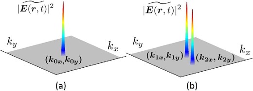
(a) Image on the |$\boldsymbol{k}$|-plane formed by a point source in the |$\boldsymbol{k_0}$| direction. (b) Images formed by two independent point sources. (Color online)
As described above, the angular resolution is given by the overall size of the antenna array, while the field of view is determined by the spacing between the antenna elements. We can thus design the configuration of the spatial FFT interferometer appropriately according to the purpose of the observation.
Most of the traditional Fourier synthesis telescopes in use today were designed to obtain fine images of radio sources using a relatively small number of antennas by choosing minimum-redundancy baselines or an arbitrary configuration of antennas. They are indirect imaging systems that use correlators and integrators. On the other hand, the spatial FFT interferometer, in which each antenna element is fixed in the maximum redundancy position, generates real-time images of radio sources at the Nyquist sampling rate. Moreover, an N-element spatial FFT interferometer requires Nlog2N multipliers, while an N-element Fourier synthesis interferometer requires N(N − 1) correlators. This means that the spatial FFT type is more economical than the correlator type when the number of elements N is large (Daishido et al. 1984).
2.2 Nasu telescope array
The Nasu telescope array is located at the Jiyu-Gakuen Nasu Farm in Tochigi Prefecture, 160 km north of Tokyo, at latitude |${36}^\circ {55^{\prime }41{_{.}^{\prime\prime}}3}$| N and longitude |$139^{\circ }{58^{\prime }54{_{.}^{\prime\prime}}3}$| E. The telescope is a one-dimensional array of eight antennas with a spacing of 21 m, aligned from east to west (E–W). The main part of each antenna is a spherical dish with a diameter of 20 m. A photograph of the 20 m antennas is shown in figure 2. The radius of curvature and the aperture diameter are both 20 m; that is, each antenna is a 60° spherical cap. For an incoming radio wave, the spherical surface of the main reflector and a Gregorian sub-reflector form a focal point at the input of the feed horn (see figure 3). The asymmetrical 3D surface of the sub-reflector was specially designed to compensate for the aberrations caused by the spherical reflector (Daishido et al. 2000).
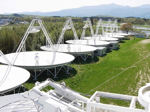
Nasu telescope array with 20 m spherical antennas at the Jiyu-Gakuen Nasu Farm. (Color online)
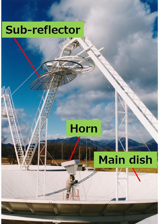
Principal parts of each antenna: main dish, sub-reflector, and feed horn. (Color online)
The main dish is fixed on the ground, whereas the sub-reflector and feed horn can be moved mechanically. The sub-reflector is located 5° from the vertex axis of the spherical reflector, and thus the elevation angle is fixed at 85°. By rotating the sub-reflector synchronously with the feed horn in azimuth, the antenna covers the sky area in a declination zone of 32° ≤ δ ≤ 42°, which is 7.0% of the entire sky.
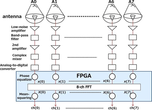
Block diagram of the Nasu telescope array including the data processing system. (Color online)
The main parameters of the Nasu telescope array are summarized in table 1.
Main parameters of the Nasu telescope array.
| Location | Latitude |$36^{\circ }{55^{\prime }41{_{.}^{\prime\prime}}3}$| N |
|---|---|
| Longitude |$139^{\circ }{58^{\prime }54{_{.}^{\prime\prime}}3}$| E | |
| Number of antennas | Eight with 21 m spacing (E–W) |
| Main reflector | Fixed 20 m spherical dish |
| Sub-reflector | Asymmetrical Gregorian type |
| Angular resolution | 0|${{_{.}^{\circ}}}$|1 (E–W) |
| Field of view (HPBW) | 0|${{_{.}^{\circ}}}$|8 |
| Declination coverage | 32° ≤ δ ≤ 42° |
| Frequency range | 1.415 ± 0.01 GHz |
| Nyquist frequency | 20 MHz |
2.3 Data analysis
The directivity of the spatial FFT interferometer is determined by the configuration of the antenna array. On the basis of the characteristics of the directivity pattern, two analysis methods have been developed: one is direct imaging and the other is correlation analysis.
2.3.1 Directivity patterns
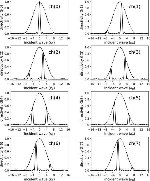
Normalized directivity pattern G(k) for each ch(k) (k = 0, 1, 2, …, 7) as a function of κ0. We assume here that |$\boldsymbol{k_0}$| is parallel to |$\boldsymbol{d}$| and d = 2a. The solid line shows the antenna pattern for each ch(k) and the broken line shows that of a single dish.
2.3.2 Direct imaging
A direct image can be obtained by making a contour map on the array block of ch(k) in equation (9). Figure 6 shows an example of a direct image obtained from the bright radio source 4C 33.57 (1.1 Jy at 1.4 GHz; Condon et al. 1998). As shown in figure 6a, the same two sets of ch(k) reduce the complexity of the folded pattern arising from the Fourier transformation. Furthermore, we can obtain a clearer image, as shown in figure 6b by masking the unnecessary part of the array before making the contour map.
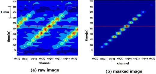
Example of direct image produced by the bright radio source 4C 33.57 (1.1 Jy at 1.4 GHz). The integration time of ch(k) is 0.6 s. (a) Raw image appearing in the same two sets of ch(k). (b) Masked view of the same image. (Color online)
In principle, the direct imaging of a radio source shows intensity variations with a short duration. For this purpose, however, an accurate calibration of the image is crucial, although the optimum method that should be used is still under investigation. Nevertheless, we can apply direct imaging to distinguish artificial noise, such as radio-frequency interference, from genuine astronomical radio signals. Direct imaging cannot be applied to very faint radio sources.
2.3.3 Correlation analysis
An example of three hours of data analyzed by the pattern-matching method is shown in figure 7. The upper figure shows the raw data of ch(0). The middle figure shows the reduced SNR of the eight-channel output data. SNR peaks larger than 7 are marked with a small circle, and the values shown at the peaks are the observed SNR. The lower figure shows the expected flux density of the radio sources listed in the NVSS catalog, taking account of the difference in the declinations between the source and the antenna positions. We obtained good agreement between the expected and observed source distributions and their intensities.
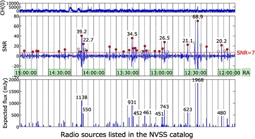
Example of three hours of data analyzed by the pattern-matching method. The upper figure shows the raw data of ch(0). The middle figure shows the combined SNR of the eight-channel output data. SNR peaks larger than 7 are marked with a small circle; the figures by the peaks are the observed SNR. Peaks with an open circle show the side lobe from strong sources. The lower figure shows the expected flux density of the radio sources listed in the NRAO VLA Sky Survey (NVSS) catalog (Condon et al. 1998) taking account of the difference in the declinations between the source and the antenna position. (Color online)
The observed one-sigma noise level was ∼20 mJy when the averaging time of ch(k) was 0.6 s. Thus, this method is effective even for rather weak radio sources.
3 Observations and results for V404 Cygni
The Nasu telescope array started an observation run on 2015 May 18, monitoring the sky region inside the declination zone of 33|${{_{.}^{\circ}}}$|8 ± 0|${{_{.}^{\circ}}}$|4 in the drift-scan mode, in which the telescope scans the sky around a selected declination as the Earth rotates. V404 Cygni is located at |${20^{\rm h}24^{\rm m}03{_{.}^{\rm s}}83}$| in right ascension (RA) and 33|${{_{.}^{\circ}}}$|9 in declination (Dec); thus, this source was within our survey area.
Figure 8 shows the daily records of the one-hour SNR data calculated by the correlation analysis method. In the plot, the horizontal axis shows the RA of the target sky region. Four days of data from 2015 June 19 to 22 are plotted here to demonstrate how to find substantial changes in the brightness among the daily records. On 2015 June 21, 17:24 UT, we found a significant peak at a position near V404 Cygni, although on June 20, 17:28 UT, we could not observe any noticeable signal in the vicinity. A nearby radio source, QSO J2025+337, whose flux density is 1268 mJy at 1.4 GHz, was chosen as a calibrator (Condon et al. 1998). The calibrated flux density of the detected signal on June 21 was 313 ± 30 mJy (Tsubono et al. 2015a). Since the center position of V404 Cygni and the calibrator is almost on the observation line, the difference in directivity was not considered here. The daily variation of the detected flux density during the two months from 2015 May 18 (MJD 57160) to July 18 UT (MJD 57221), which includes the period of the V404 Cygni outburst, is plotted in figure 9. Except for the 10 d from 2015 June 21 (MJD 57194) to June 30 UT (MJD 57203), the detected signal was below the detection limit.

Daily records of the one-hour SNR data from 2015 June 19 to June 22. An enlarged view of part of the figure is also shown. Peaks with an open circle show the side lobe from strong sources. On June 21, 17:24 UT, we found a significant peak at a position near V404 Cygni, although on June 20, 17:28 UT, we could not observe any noticeable signal in the vicinity. A nearby radio source, QSO J2025+337, was chosen as a calibration star, whose flux density is 1268 mJy at 1.4 GHz (Condon et al. 1998). (Color online)
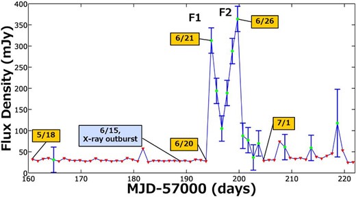
Daily variation of the detected flux density around V404 Cygni during the two months from 2015 May 18 (MJD 57160) to July 18 UT (MJD 57221), including the period of the V404 Cygni outburst. Except for the 10 d from June 21 (MJD 57194) to June 30 UT (MJD 57203), the detected signal was below the detection limit (filled red triangle). These detection limits can sometimes be high, mainly due to bad weather at the observation site. The date of the X-ray outburst is also shown here. (Color online)
On 2015 June 21, 17:24 UT, we found a significant peak of 313 ± 30 mJy at the position of V404 Cygni. Then, the observed flux density decreased to 105 ± 30 mJy on June 23, 17:17 UT. However, the flux density recovered from that point and increased to 364 ± 30 mJy on June 26, 17:05 UT. On June 27, 17:01 UT, we observed fast decay of the intensity (Tsubono et al. 2015b). After this rapid decay, the flux density seemed to slowly decay. These characteristics appeared to be similar to those of the radio decay curve reported for the 1989 outburst of V404 Cygni (Han & Hjellming 1992).
4 Discussions
As mentioned in section 1, Barthelmy et al. (2015) and Negoro et al. (2015) reported that Swift-BAT and MAXI-GSC captured the huge X-ray outburst, which preceded the radio outburst, in the black hole X-ray binary object V404 Cygni. After this X-ray observation, and in response to the alert about its detection, follow-up observations were performed by ground-based telescopes, including not only radio telescopes but also other telescopes such as optical telescopes. On the other hand, fortunately, we had been monitoring the region at a declination line of 33|${{_{.}^{\circ}}}$|8 ± 0|${{_{.}^{\circ}}}$|4, at which V404 Cygni is located, every day since 2015 May 18, which was almost one month before the X-ray outburst and during which time V404 Cygni was in the quiescent state in the 1.4 GHz radio band.
Although an accurate understanding of the flux increase in the flaring phase of non-thermal synchrotron emission is essential for investigating the coupling between the accretion state and the jet ejection mechanism, which is one of the most important questions, it is quite difficult to obtain early-stage information of the flare, especially for radio observation, not only at higher frequencies but also at lower frequencies. Because of their smaller field of view (FoV), most radio telescopes have not performed unbiased surveys, but have carried out follow-up observations of transient phenomena triggered by X-ray/γ-ray observations by all-sky monitoring satellites.
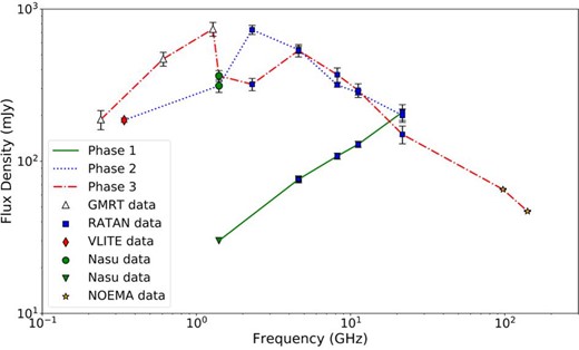
Radio spectra of V404 Cygni in the quiescent (phase 1; solid line) and outburst phases (phases 2 and 3: dotted and dashed lines, respectively) at 1.4 GHz. Each color indicates radio spectra obtained in different phases. The filled green triangle shows an upper limit for the 1.4 GHz radio flux density in phase 1. Additionally, the filled red diamond shows the 0.34 GHz radio flux density, but it was obtained more than 10 hr later compared to the other radio flux densities in phase 2. (Color online)
Multi-frequency radio data in the quiescent and outburst phases.*
| ν | S | S err | |||
|---|---|---|---|---|---|
| Epoch | (GHz) | (mJy) | (mJy) | Date | Ref. |
| Phase 1 | 1.4 | <30 | — | 2015-Jun-18.73 | (1) |
| 4.6 | 76 | 4 | 2015 Jun 18.95 | (2) | |
| 8.2 | 108 | 5 | 2015 Jun 18.95 | (2) | |
| 11.2 | 129 | 6 | 2015 Jun 18.95 | (2) | |
| 21.7 | 210 | 25 | 2015 Jun 18.95 | (2) | |
| Phase 2 | 0.34 | 186 | 6 | 2015 Jun 22.54 | (3) |
| 1.4 | 313 | 30 | 2015 Jun 21.73 | (1) | |
| 2.3 | 730 | 50 | 2015 Jun 21.94 | (2) | |
| 4.6 | 540 | 30 | 2015 Jun 21.94 | (2) | |
| 8.2 | 317 | 10 | 2015 Jun 21.94 | (2) | |
| 11.2 | 282 | 10 | 2015 Jun 21.94 | (2) | |
| 21.7 | 200 | 20 | 2015 Jun 21.94 | (2) | |
| Phase 3 | 0.24 | 188 | 27 | 2015 Jun 26.89 | (4) |
| 0.61 | 470 | 49 | 2015 Jun 26.89 | (4) | |
| 1.28 | 739 | 77 | 2015 Jun 26.89 | (4) | |
| 1.4 | 364 | 30 | 2015 Jun 26.71 | (1) | |
| 2.3 | 320 | 30 | 2015 Jun 26.93 | (2) | |
| 4.6 | 534 | 50 | 2015 Jun 26.93 | (2) | |
| 8.2 | 370 | 40 | 2015 Jun 26.93 | (2) | |
| 11.2 | 292 | 30 | 2015 Jun 26.93 | (2) | |
| 21.7 | 150 | 20 | 2015 Jun 26.93 | (2) | |
| 97.5 | 65.2 | 0.2 | 2015 Jun 26.93 | (5) | |
| 140.5 | 46.9 | 0.3 | 2015 Jun 26.93 | (5) |
*Column 1: The state of source activity. Column 2: Observed frequencies in units of of GHz. Columns 3 and 4: Flux densities and errors, in units of mJy. Column 5: Date on which each datum was obtained. Here we assume that radio data at low frequencies obtained within several hours show the same behavior. Column 6: References: (1) our observation; (2) Trushkin, Nizhelskij, and Tybulev (2015); (3) Kassim et al. (2015); (4) Chandra and Kanekar (2017); (5) Tetarenko et al. (2015).
5 Conclusion
We used the Nasu telescope array, which is a spatial FFT interferometer, to carry out daily monitoring of radio transient phenomena by drift-scan observation. This telescope makes it possible to perform observation of all right ascensions with a sensitivity of a few tens of mJy at a specific declination with a positional uncertainty of ±0|${{_{.}^{\circ}}}$|4 over a day. On the other hand, no other radio observatory allows us to conduct wide-field daily monitoring with higher sensitivity, especially in the East Asian region. Therefore, it is complementary to other radio telescopes, which can conduct not only monitoring of specific objects with high time resolution or high angular resolution, but also unbiased surveys with large FoV in other regions (e.g., CHIME/FRB Collaboration 2018).
As a successful demonstration, our daily monitoring with the Nasu telescope from one month before the outburst of V404 Cygni occurred in 2015 June allowed us to capture the detailed behavior, which showed an abrupt change in flux density caused by an outburst in the 1.4 GHz radio band. The radio light curve showed two huge outbursts that occurred during a period of 10 d, and at least the 1.4 GHz flux density during one of the two outbursts increased by more than ten times within a day, compared to the quiescent state. We have also confirmed the extreme variation of radio spectra within the short period mentioned above by collecting other radio data observed at several radio observatories. Such spectral behaviors are considered to reflect the change in the opacity of the ejected blobs associated with radio and X-ray outbursts.
Although there is room to improve the calibration issues, which is crucial for accurate measurement of the amplitude and position of radio transients, as mentioned in Thompson et al. (2017), this new type of wide-field radio telescope realized by adopting a spatial FFT technique is one of the most promising key techniques in the era of “time-domain and multi-messenger astronomy.”
Acknowledgements
We are grateful to the anonymous referee, whose suggestions improved our paper substantially. This work was supported in part by the Cooperative and Supporting Program for Research and Education in Universities of the National Astronomical Observatory of Japan (NAOJ) and by Japan Society for the Promotion of Science (JSPS) KAKENHI Grant Numbers JP15K05029 (K.T.), JP18H03721 (K.N.), and JP15H00784 (K.N.). We thank Dr. Trushkin for providing us with their RATAN-600 data.
References
