


Abstract
Recent constraints on the splashback radius around optically selected galaxy clusters from the redMaPPer cluster-finding algorithm in the literature have shown that the observed splashback radius is |${\sim}20\%$| smaller than that predicted by N-body simulations. We present analyses on the splashback features around ∼ 3000 optically selected galaxy clusters detected by the independent cluster-finding algorithm CAMIRA over a wide redshift range of 0.1 < zcl < 1.0 from the second public data release of the Hyper Suprime-Cam (HSC) Subaru Strategic Program covering ∼427 deg2 for the cluster catalog. We detect the splashback feature from the projected cross-correlation measurements between the clusters and photometric galaxies over the wide redshift range, including for high-redshift clusters at 0.7 < zcl < 1.0, thanks to deep HSC images. We find that constraints from red galaxy populations only are more precise than those without any color cut, leading to 1σ precisions of |${\sim}15\%$| at 0.4 < zcl < 0.7 and 0.7 < zcl < 1.0. These constraints at 0.4 < zcl < 0.7 and 0.7 < zcl < 1.0 are more consistent with the model predictions (≲1σ) than their |$20\%$| smaller values as suggested by the previous studies with the redMaPPer (∼2σ). We also investigate selection effects of the optical cluster-finding algorithms on the observed splashback features by creating mock galaxy catalogs from a halo occupation distribution model, and find such effects to be sub-dominant for the CAMIRA cluster-finding algorithm. We also find that the redMaPPer-like cluster-finding algorithm induces a smaller inferred splashback radius in our mock catalog, especially at lower richness, which can well explain the smaller splashback radii in the literature. In contrast, these biases are significantly reduced when increasing its aperture size. This finding suggests that aperture sizes of optical cluster finders that are smaller than splashback feature scales can induce significant biases on the inferred location of a splashback radius.
1 Introduction
Galaxy clusters are the most massive gravitationally bound structure in the Universe, which form in dark matter halos around rare high peaks in the initial density field after interactions between gravitational dynamics and baryoni process related to galaxy formation (see Allen et al. 2011; Kravtsov & Borgani 2012; Weinberg et al. 2013; Wechsler & Tinker 2018; Pratt et al. 2019; Walker et al. 2019; Vogelsberger et al. 2020, for recent reviews). The splashback radius has been proposed as a physical boundary of dark matter halos at the outskirts which separates orbiting from accreting materials as a sharp density edge, which is seen even after stacking of halos through numerical simulations (Diemer & Kravtsov 2014; More et al. 2015) and can be explained with a simple analytical model (Adhikari et al. 2014). At the splashback radius, the logarithmic derivative of density profiles is predicted to drop significantly over a narrow range of radius in the outskirts due to the piling up of materials with small radial velocities at their first orbital apocenter after infall on to the halo. The splashback radius primarily depends on the accretion rate, redshift, and halo mass (e.g., Diemer et al. 2017). The secondary infall models with the spherical collapse model (Gunn & Gott 1972) predict such a sharp density edge analytically (e.g., Fillmore & Goldreich 1984; Bertschinger 1985; Adhikari et al. 2014; Shi 2016). Furthermore, the splashback features have been investigated from various aspects with simulations (Oguri & Hamana 2011; Mansfield et al. 2017; Diemer 2017; Okumura et al. 2018; Sugiura et al. 2020; Xhakaj et al. 2019), including dark energy (Adhikari et al. 2018), modified gravity (Adhikari et al. 2018; Contigiani et al. 2019b), and self-interacting dark matter (Banerjee et al. 2020).
Observationally, the splashback feature has been detected and constrained statistically for galaxy clusters selected by the optical cluster-finding algorithm redMaPPer (Rykoff et al. 2012, 2014, 2016; Rozo & Rykoff 2014; Rozo et al. 2015a, 2015b) through cross-correlation measurements between clusters and galaxies (More et al. 2016; Baxter et al. 2017; Chang et al. 2018; Shin et al. 2019) or weak lensing measurements (Chang et al. 2018) with high precision thanks to a large number of optically selected clusters. Less-precise measurements have also been done for clusters selected by the Sunyaev–Zel’dovich effect (Zürcher & More 2019; Shin et al. 2019) or X-ray flux (Umetsu & Diemer 2017; Contigiani et al. 2019a). We note that the signal-to-noise ratios for weak lensing measurements are smaller than those for cluster–galaxy cross-correlation measurements to constrain the splashback feature. It is important to validate theoretical predictions against observed splashback features with the help of weak-lensing mass calibrations, where weak-lensing measurements constrain the mass-observable relation mainly from their amplitudes, instead of the location of the splashback radius imprinted in lensing measurements. Interestingly, the high-precision measurements of the splashback radius for the redMaPPer clusters (More et al. 2016; Baxter et al. 2017; Chang et al. 2018) from the Sloan Digital Sky Survey (SDSS) or the Dark Energy Survey (DES) data show that their observed splashback radius from cluster–galaxy cross-correlation measurements is smaller than expected from N-body simulations under the standard Λ cold dark matter (ΛCDM) cosmology at the level of |$20\% \pm 5\%$|. Shin et al. (2019) also show a similar trend at the ∼2σ level for the redMaPPer clusters at more massive mass scales.
One of the possible origins of the inconsistency is some systematics in the optical cluster-finding algorithm, such as projection effects in optical cluster-finding algorithms for which non-member galaxies along the line-of-sight as member galaxies in optical richness estimation (e.g., Cohn et al. 2007; Zu et al. 2017; Busch & White 2017; Costanzi et al. 2019; Sunayama & More 2019). In particular, Busch and White (2017) and Sunayama and More (2019) investigated projection effects on the splashback features with a simplified redMaPPer-like optical cluster-finding algorithm in the Millennium Simulation (Springel et al. 2005). However, their cluster abundance densities in the simulations is ∼3 times larger than observations as a function of richness, mainly due to the use of a mock galaxy population from a semi-analytical model, which could lead to the overestimation of the projection effects. Also, Busch and White (2017) and Sunayama and More (2019) did not analyze their mock data by fitting the model profile proposed in Diemer and Kravtsov (2014) to the observed projected cross-correlation function, thus not entirely mimicking the procedure adopted in observational studies (e.g., More et al. 2016; Chang et al. 2018). Therefore, we can improve this aspect in mock simulation analyses to investigate possible bias effects from optical cluster-finding algorithms by more closely resembling the comparison procedure in the observations. Thus, further independent investigation would be useful to confirm whether the inconsistency is caused by artifacts due to optical cluster-finding algorithms or not.
The distribution of galaxies after magnitude or color cuts in observations is expected to have the same splashback radius as dark matter distribution to the first-order approximation, unless such cuts select particular orbits of recently accreted galaxies in clusters due to fast quenching effects, for instance. The difference between dark matter and subhalos, where galaxies should reside, can be caused by dynamical friction (Chandrasekhar 1943) that affects subhalos with a ratio of mass to host halo mass Msub/Mhost ≳ 0.01 (Adhikari et al. 2016) to decrease splashback radii significantly (|${\gtrsim}5\%$|) compared to the dark matter. In observations, fainter galaxies are expected to live in less-massive subhalos, and thus dynamical friction effects are smaller. Hence, fainter galaxies are expected to have splashback radii closer to those for the dark matter. However, relations between subhalo masses and galaxy luminosities (including scatter between them) have not been fully understood. Dynamical friction effects on splashback radii are investigated in the literature (More et al. 2016; Chang et al. 2018; Zürcher & More 2019) with different absolute magnitude thresholds. However, a magnitude dependence of splashback radii for massive clusters has not been detected even with smaller error bars in More et al. (2016) at a |${\lesssim}5\%$| precision level, even though a |${\gtrsim}5\%$| shift of splashback radii is expected in simulations especially for more massive subhalos when selecting subhalos with maximum circular velocities throughout their entire history to reproduce galaxy abundances in observations (More et al. 2016; Chang et al. 2018). The scatter between the maximum circular velocities (or subhalo masses) and galaxy luminosities could wash out dynamical friction effects (More et al. 2016). It would be interesting to explore dynamical friction effects with an independent optical cluster-finding algorithm and fainter galaxy samples.
One of the most striking features within galaxy clusters is the presence of a larger number of red and elliptical galaxies with little ongoing star formation (Oemler 1974; Dressler 1980; Dressler & Gunn 1983; Balogh et al. 1997; Poggianti et al. 1999), exhibiting a tight relation in the color–magnitude diagram (e.g., Stanford et al. 1998). These quenching effects are expected from intra-cluster astrophysical processes including tidal disruption, harassment, strangulation (Larson et al. 1980), and ram-pressure stripping (Gunn & Gott 1972), or from the age-matching model (e.g., Hearin et al. 2014) which employs expectations that galaxies in larger overdensities form earlier. Quenching of satellite galaxies at the outskirts of galaxy clusters has been investigated (e.g., Wetzel et al. 2013; Fang et al. 2016; Zinger et al. 2018; Adhikari et al. 2019). The splashback radius separates orbiting from accreting galaxies as the physical boundary of halos, and thus investigating relations between the splashback and quenching features around clusters over a wide range of redshift would be informative to constrain galaxy formation and evolution physics.
The Hyper Suprime-Cam Subaru Strategic Program (HSC-SSP) is a wide-field optical imaging survey (Miyazaki et al. 2012, 2015, 2018; Furusawa et al. 2018; Kawanomoto et al. 2018; Komiyama et al. 2018) with a 1.77 deg2 field-of-view camera on the 8.2 m Subaru telescope. The HSC survey is unique in its combination of depth and high-resolution image quality, which allows us to detect galaxy clusters over a wide redshift range up to zcl ∼1 and to investigate their splashback features with photometric galaxies down to fainter apparent magnitudes compared to other ongoing wide-field surveys, although the survey area is smaller than those of other imaging surveys in the literature (More et al. 2016; Chang et al. 2018).
In this paper, we present constraints on the splashback features of the HSC optically-selected clusters in the cluster redshift range of 0.1 ≤ zcl ≤ 1.0 and the richness range of 15 ≤ N ≤ 200 detected by the independent cluster-finding algorithm CAMIRA (Oguri 2014) from the HSC-SSP second public data release (Aihara et al. 2019). The main difference between the redMaPPer and CAMIRA cluster-finding algorithms is that CAMIRA subtracts the background galaxy levels to estimate the richness in cluster selection locally, but redMaPPer does this globally. Moreover, CAMIRA employs a larger aperture size (≃1 h−1 Mpc in physical coordinates) independent of richness values in cluster selections, whereas redMaPPer uses a smaller richness-dependent aperture (<1 h−1 Mpc in physical coordinates for almost all clusters). To constrain the splashback features, we measure the projected cross-correlation function between the HSC CAMIRA clusters and the HSC photometric galaxies. We investigate the dependence of splashback features for the CAMIRA clusters on cluster redshift, richness, galaxy magnitude limit, and galaxy color. We compare results from a model fitting to the projected cross-correlation measurements with predictions from the halo–matter cross-correlation function in Dark Emulator (Nishimichi et al. 2019), which is constructed from a suite of high-resolution N-body simulations, and the mass–richness relation of the HSC CAMIRA clusters (Murata et al. 2019) constrained by stacked weak gravitational lensing and abundance measurements with a pipeline developed in Murata et al. (2018). We also investigate how projection effects could bias splashback feature measurements using a simplified estimation of the impact of the optical cluster-finding algorithms partly following approaches presented in Busch and White (2017) and Sunayama and More (2019). For this purpose, we construct mock galaxy catalogs by populating galaxies in N-body simulations with a halo occupation distribution (HOD; Zheng et al. 2005) model to match cluster abundance densities and lensing profiles to observations approximately.
The structure of this paper is as follows. In section 2, we describe the Subaru HSC data and catalogs used in our splashback feature analysis and the projected cross-correlation function measurements between the HSC clusters and galaxies. In section 3, we summarize a model fitting method with a parametric density profile from Diemer and Kravtsov (2014) to constrain splashback features from the projected cross-correlation measurements. In section 4, we show the resulting constraints on the splashback features and compare them with model predictions. We discuss the robustness of our results in section 5. Finally, we conclude in section 6.
Throughout this paper, we use natural units where the speed of light is set equal to unity, c = 1. We use |$M \equiv M_{\rm 200m}=4 \pi (R_{\rm 200m})^3 \bar{\rho }_{\rm m0} \times 200/3$| for the halo mass definition, where R200m is the three-dimensional comoving radius within which the mean mass density is 200 times the present-day mean mass density. In this paper, we use a radius and density in comoving coordinates rather than in physical coordinates, unless otherwise stated. We adopt the standard flat ΛCDM model as the fiducial cosmological model with cosmological parameters from the Planck15 result (Planck Collaboration 2016): Ωb0 h2 = 0.02225 and Ωc0 h2 = 0.1198 for the density parameters of baryon and cold dark matter, respectively, ΩΛ = 0.6844 for the cosmological constant, σ8 = 0.831 for the normalization of the matter fluctuation, and ns = 0.9645 for the spectral index. We employ the convention used in More et al. (2015, 2016) for the splashback radius, where |$r_{\rm sp}^{\rm 3D}$| and |$R_{\rm sp}^{\rm 2D}$| correspond to the locations of the steepest logarithmic derivative of the radially averaged density profiles after stacking of halos in the three-dimensional or projected space, respectively, due to its accessibility in observations.
2 Data and measurement
2.1 HSC-SSP survey
HSC is a wide-field prime focus camera with a |${1{_{.}^{\circ}}5}$| diameter field-of-view mounted on the 8.2 m Subaru telescope (Miyazaki et al. 2012, 2015, 2018; Furusawa et al. 2018; Kawanomoto et al. 2018; Komiyama et al. 2018). With its unique combination of a wide field-of-view, a large aperture of the primary mirror, and excellent image quality, HSC can detect relatively higher redshift clusters and fainter galaxies compared with other ongoing wide-field surveys. To fully exploit its survey power, the HSC-SSP (Aihara et al. 2018a, 2018b, 2019) conducted a multi-band wide-field imaging survey over six years with 300 nights. The HSC-SSP survey consists of three layers: Wide, Deep, and UltraDeep. The Wide layer aims at covering 1400 deg2 of the sky with five broad-bands (grizy) and a 5σ point-source depth of r ∼ 26. Bosch et al. (2018) describes the software pipelines used to reduce the data.
In this paper, we use HSC cluster and galaxy catalogs based on the photometric data in the Wide layer with the five broad-bands in the HSC-SSP second Public Data Release (PDR2; Aihara et al. 2019). PDR2 includes the datasets from 2014 March through 2018 January, about 174 nights in total. The median seeing for i-band images is |$\sim {0_{.}^{\prime \prime }6}$| in terms of the point-spread function (PSF) full width at half-maximum. The typical seeing, 5σ depth for extended sources, and saturation magnitude for z-band images in the Wide layer are |${0_{.}^{\prime \prime }68}$|, 25.0 mag, and 17.5 mag, respectively, after averaging over the entire survey area included in PDR2 (Aihara et al. 2019).
2.2 HSC CAMIRA cluster catalog
We use the CAMIRA (Cluster-finding Algorithm based on Multi-band Identification of Red-sequence gAlaxies) cluster catalog from the HSC-SSP Wide dataset in PDR2, which was constructed using the CAMIRA algorithm (Oguri 2014). This catalog is an updated version of the one presented in Oguri et al. (2018) based on the first-year HSC-SSP dataset. The CAMIRA algorithm is a red-sequence cluster finder based on a stellar population synthesis model (Bruzual & Charlot 2003) to predict colors of red-sequence galaxies at a given redshift and to compute likelihoods of being red-sequence galaxies as a function of redshift. The stellar population synthesis model in the CAMIRA algorithm is calibrated with spectroscopic galaxies to improve its accuracy (Oguri et al. 2018). The richness in the CAMIRA algorithm corresponds to the number of red cluster member galaxies with stellar mass M* ≳ 1010.2 M⨀ (roughly corresponding to the luminosity range of L ≳ 0.2 L*) within a circular aperture with a radius R ≲ 1 h−1Mpc in physical coordinates. Unlike the redMaPPer algorithm (Rykoff et al. 2012), the CAMIRA algorithm does not employ a richness-dependent aperture radius to define the richness. The HSC images are deep enough to detect cluster member galaxies down to M* ∼ 1010.2 M⨀ even at redshift zcl ∼ 1, which allows us to detect such high-redshift clusters reliably without the richness incompleteness correction. The algorithm employs a spatially-compensated filter that subtracts the background level locally in deriving the richness. CAMIRA defines cluster centers as locations of the identified brightest cluster galaxies (BCGs). The bias and scatter in photometric cluster redshifts of Δzcl/(1 + zcl) are shown to be better than 0.005 and 0.01, respectively, with 4σ clipping over most of the redshift range by using available spectroscopic redshifts of BCGs (Oguri et al. 2018). We use the cluster catalog after applying bright-star masks for grizy-bands presented in Aihara et al. (2019).
The catalog contains 3316 clusters at 0.1 ≤ zcl ≤ 1.0 with the richness 15 ≤ N ≤ 200 with almost uniform completeness and purity over the sky region. We divide the whole sample into subsamples with different redshift and richness selections to investigate redshift and richness dependences of splashback features. The sample selections and characteristics are shown in table 1. The total area for this version of the HSC CAMIRA clusters is estimated to be 427 deg2. In addition to the cluster catalog, we use a random cluster catalog with the same redshift and richness distributions as the data in the same footprint. There are 100 times as many random points as real clusters to measure projected cross-correlation functions with galaxies accurately.
Sample selections for the HSC CAMIRA clusters and their characteristics.*
| Selection | |||||||
|---|---|---|---|---|---|---|---|
| Characteristic | Full | Low-z | Mid-z | High-z | Low-N | Mid-N | High-N |
| z cl, min | 0.1 | 0.1 | 0.4 | 0.7 | 0.1 | 0.1 | 0.1 |
| z cl, max | 1.0 | 0.4 | 0.7 | 1.0 | 1.0 | 1.0 | 1.0 |
| 〈zcl〉 | 0.57 | 0.26 | 0.55 | 0.83 | 0.60 | 0.54 | 0.49 |
| N min | 15 | 15 | 15 | 15 | 15 | 20 | 30 |
| N max | 200 | 200 | 200 | 200 | 20 | 30 | 200 |
| 〈N〉 | 23 | 25 | 22 | 21 | 17 | 24 | 40 |
| Number of clusters | 3316 | 968 | 1140 | 1208 | 1774 | 1067 | 475 |
| 〈M200m〉 [h−11014 M⨀] | |$1.72^{+0.08}_{-0.07}$| | |$1.71^{+0.07}_{-0.07}$| | |$1.93^{+0.09}_{-0.08}$| | |$1.51^{+0.13}_{-0.13}$| | |$1.23^{+0.06}_{-0.06}$| | |$1.78^{+0.08}_{-0.08}$| | |$3.32^{+0.14}_{-0.15}$| |
| 〈R200m〉 [h−1 Mpc] | |$1.33^{+0.02}_{-0.02}$| | |$1.33^{+0.02}_{-0.02}$| | |$1.38^{+0.02}_{-0.02}$| | |$1.27^{+0.04}_{-0.04}$| | |$1.19^{+0.02}_{-0.02}$| | |$1.34^{+0.02}_{-0.02}$| | |$1.65^{+0.02}_{-0.03}$| |
| |$r_{\rm sp, model}^{\rm 3D}\ [h^{-1}\:\mbox{Mpc}]$| | |$1.61^{+0.01}_{-0.01}$| | |$1.61^{+0.01}_{-0.01}$| | |$1.63^{+0.01}_{-0.01}$| | |$1.45^{+0.03}_{-0.02}$| | |$1.41^{+0.01}_{-0.01}$| | |$1.62^{+0.01}_{-0.01}$| | |$1.92^{+0.01}_{-0.01}$| |
| |$\frac{ {d}\ln \xi _{\rm 3D} }{ {d}\ln r }|_{r=r_{\rm sp}^{\rm 3D}, {\rm model}}$| | |$-3.20^{+0.03}_{-0.03}$| | |$-3.11^{+0.03}_{-0.03}$| | |$-3.25^{+0.03}_{-0.03}$| | |$-3.27^{+0.05}_{-0.05}$| | |$-3.21^{+0.04}_{-0.04}$| | |$-3.28^{+0.03}_{-0.03}$| | |$-3.34^{+0.03}_{-0.03}$| |
| |$R_{\rm sp, model}^{\rm 2D}\ [h^{-1}\:\mbox{Mpc}]$| | |$1.12^{+0.01}_{-0.02}$| | |$1.07^{+0.03}_{-0.02}$| | |$1.16^{+0.01}_{-0.01}$| | |$1.07^{+0.04}_{-0.03}$| | |$0.99^{+0.01}_{-0.01}$| | |$1.13^{+0.01}_{-0.02}$| | |$1.39^{+0.02}_{-0.01}$| |
| |$\frac{ {d}\ln \xi _{\rm 2D} }{ {d}\ln R }|_{R=R_{\rm sp}^{\rm 2D}, {\rm model}}$| | |$-1.72^{+0.02}_{-0.02}$| | |$-1.67^{+0.01}_{-0.01}$| | |$-1.75^{+0.01}_{-0.01}$| | |$-1.75^{+0.03}_{-0.03}$| | |$-1.69^{+0.02}_{-0.02}$| | |$-1.75^{+0.02}_{-0.02}$| | |$-1.82^{+0.01}_{-0.01}$| |
*We define each cluster sample by zcl, min, zcl, max, Nmin, and Nmax, and 〈zcl〉 and 〈N〉 give the mean values of cluster redshift and richness. We show the constraints for each sample on mean mass and R200m values, and the model predictions for the splashback feature from the mass–richness relation in Murata et al. (2019) and the halo emulator in Nishimichi et al. (2019) as described in appendix 1. We note that we use the halo–matter cross-correlation function for these model predictions and we compare our model predictions with model calculation methods in the literature in appendix 2. We show the median and the 16th and 84th percentiles of the model predictions using the fiducial results of the mass–richness relation in Murata et al. (2019) with the Planck cosmology.
We also employ the HSC CAMIRA member galaxy catalog to define color cuts to separate red and blue galaxies at each cluster redshift, following a red-sequence-based method in Nishizawa et al. (2018), which we will use to investigate galaxy color dependence of splashback features in subsection 4.3. These member galaxies are red-sequence galaxies identified by the CAMIRA algorithm as described in Oguri (2014). We use all the red-sequence member galaxies for clusters with richness N ≥ 10 to define separation criteria for red and blue galaxies (see Nishizawa et al. 2018). The total number of member galaxies is 331168 at 0.1 ≤ zcl ≤ 1.0.
We use the richness–mass relation presented in Murata et al. (2019) to model splashback features for each redshift and richness selection, as described in appendix 1. Murata et al. (2019) constrained the richness–mass relation P(N|M, z) from the stacked weak gravitational lensing profiles from the HSC-SSP first-year shear catalog (Mandelbaum et al. 2018a, 2018b) and the photometric redshift catalog (Tanaka et al. 2018), and abundance measurements for the HSC CAMIRA clusters with 0.1 ≤ zcl ≤ 1.0 and 15 ≤ N ≤ 200. We note that Murata et al. (2019) used the previous version of the HSC CAMIRA cluster catalog from the first-year dataset presented in Oguri et al. (2018). The richness differences from the updated version for matched clusters in both the versions are negligibly small compared to the scatter values in the mass–richness relation. Murata et al. (2019) also constrained the off-centering between real cluster centers and the identified BCGs for the HSC CAMIRA clusters from the stacked lensing profiles. In section 3, we use these results as inputs to our prior distributions of off-centering parameters to marginalize over its effect on the projected cross-correlation measurements between the HSC CAMIRA clusters and photometric galaxies.
2.3 HSC photometric galaxy catalog
We use the photometric galaxy catalog from PDR2 in Aihara et al. (2019) to measure projected cross-correlation functions with the clusters. We employ |$\tt {cmodel}$| magnitudes (see Bosch et al. 2018, for more details) for total z-band magnitudes in absolute-magnitude cuts (Nishizawa et al. 2018) because the z-band magnitude is more suitable for measurements of brightness of high-redshift galaxies at zcl ∼ 1.0 than the i-band magnitude used in the literature for lower redshifts (e.g., More et al. 2016), given the wavelength of 4000 Å break at such high redshifts . We define magnitudes in the other broad-bands such that we derive colors of individual galaxies with afterburner aperture photometries (Bosch et al. 2018; Oguri et al. 2018; Nishizawa et al. 2018) to avoid inaccurate photometries in crowded regions, including cluster centers, due to a failure of the deblender in such regions. The HSC pipeline measures the afterburner aperture photometries after the pipeline matches the PSF sizes on the undeblended images between all five broad-bands to have accurate colors even in crowded regions. We use the target PSF size of |${1_{.}^{\prime \prime }3}$| and the aperture size of |${1_{.}^{\prime \prime }5}$| in diameter (|$\tt {undeblended\_convolvedflux\_3\_15}$|) for PDR2 (Aihara et al. 2019).
We apply the following quality cuts to select galaxies for the measurements. First, we select galaxies observed in all five broad-bands by imposing cuts in the number of exposure images used to create a co-add image for each galaxy, as described below. While the nominal definition of the full depth are four exposures for gr bands and six for izy bands in the Wide layer of PDR2, we adopt the following relaxed conditions to avoid gaps in the galaxy distribution due to CCD gaps.
|$\tt {[gr]\_inputcount\_value}\ge 2$|
|$\tt {[izy]\_inputcount\_value}\ge 4$|
Secondly, we apply the following basic flag cuts for all five broad-bands to remove galaxies that can be affected by bad pixels or poor photometric measurements. We also focus only on unique detections(see Aihara et al. 2018b, 2019).
|$\tt {[grizy]\_pixelflags\_edge}=\tt {False}$|
|$\tt {[grizy]\_pixelflags\_interpolatedcenter}=\tt {False}$|
|$\tt {[grizy]\_pixelflags\_crcenter}=\tt {False}$|
|$\tt {[grizy]\_cmodel\_flag}=\tt {False}$|
|$\tt {[grizy]\_undeblended\_convolvedflux\_3\_15\_flag}=\tt {False}$|
|$\tt {isprimary}=\tt {True}$|
Thirdly, we use galaxies with z-band cmodel magnitude brighter than 24.5 mag after dust extinction corrections (|$\tt {a\_z}$|), flux signal-to-noise ratio larger than 5, and with an i-band star-galaxy separation parameter indicating extended sources. We use the i-band star–galaxy separation because i-band images are taken in better seeing conditions on average. We also place weak constraints on the ri-band magnitudes as r < 28 mag and i < 28 mag to remove artifacts.
|$\tt {z\_cmodel\_mag - a\_z}<24.5$|
|$\tt {z\_cmodel\_flux} > 5\times \tt {z\_cmodel\_fluxsigma}$|
|$\tt {i\_extendedness\_value}=1$|
We then apply bright-star mask cuts for all five broad-bands.
|$\tt {[grizy]\_mask\_s18a\_bright\_objectcenter}$|=False
We use angular positions (|$\tt {ra}$| and |$\tt {dec}$|) of the galaxies for the measurements. The catalog after these quality cuts includes 48882039 galaxies for analyses in subsections 4.1 and 4.2. Also, we apply absolute-magnitude cuts for additional galaxy selections in each cluster redshift bin, as described in subsection 2.4.
We note that these quality cuts for the galaxy catalog are the same as those used for constructing the cluster catalog from PDR2 in subsection 2.2 except that |$\tt {z\_cmodel\_mag - a\_z}<24.0$| and |$\tt {z\_cmodel\_magsigma}<0.1$| are used for the galaxies instead of |$\tt {z\_cmodel\_mag - a\_z}<24.5$| and |$\tt {z\_cmodel\_flux} >5\times \tt {z\_cmodel\_fluxsigma}$|. In the former case, the catalog includes 31719028 galaxies. These cuts are almost the same as those used for constructing the cluster catalog from the HSC first-year dataset presented in Oguri et al. (2018). Nishizawa et al. (2018) also used similar quality cuts for the HSC first-year datasets. We employ the catalog with these cuts for analyses with red and blue galaxies in subsection 4.3 because we define red and blue galaxies by the CAMIRA member galaxy catalog with the same galaxy quality cuts.
We also employ a random catalog for the photometric galaxies from PDR2 with the same quality cuts when related quantities are available for the random catalog in PDR2. Specifically, we do not apply the |$\tt {cmodel\_flag}$|, |$\tt {undeblended\_convolvedflux\_3\_15\_flag}$|, |$\tt {cmodel\_mag}$|, |$\tt {cmodel\_fluxsigma}$|, |$\tt {cmodel\_magsigma}$|, or |$\tt {extendedness\_value}$| cuts described above for the random catalog. The input number density of random points is 100 points arcmin−2 when constructing the random catalog (Aihara et al. 2019). Because we use the conservative magnitude and flux signal-to-noise ratio (or magnitude error) cuts for the galaxy catalogs compared with the detection limits for the z-band described in subsection 2.1, the footprint of the random catalog follows the data footprint. We use this random galaxy catalog for measurements of projected cross-correlation functions in subsection 2.4.
2.4 Projected cross-correlation measurement
We apply an absolute-magnitude cut Mz − 5log10h < −18.8 for our fiducial galaxy selection in subsection 4.1. This absolute magnitude limit corresponds to an apparent magnitude limit of z-mag = 24.5 at zcl = 1.0. We use the mean redshift value zcl, i for each subsample to convert the absolute magnitude to each apparent magnitude limit. We employ absolute-magnitude cuts in order to make fair comparisons between results at different redshifts. Nishizawa et al. (2018) employed a similar absolute-magnitude cut on z-band magnitude with the first-year HSC-SSP datasets. In subsection 4.2, we also use several different absolute-magnitude cuts to investigate how constraints on the splashback feature change mainly to investigate possible dynamical friction effects. Furthermore, in subsection 4.3, we apply a red-sequence-based red and blue separation cut in Nishizawa et al. (2018) for the photometric galaxies with a slightly brighter absolute-magnitude cut, Mz − 5log10h < −19.3, to check the dependence of splashback features on galaxy colors.
We then estimate the covariance describing the statistical uncertainties of the projected cross-correlation measurements from the jackknife method (e.g., Norberg et al. 2009) following the literature (More et al. 2016; Baxter et al. 2017; Chang et al. 2018; Nishizawa et al. 2018; Shin et al. 2019; Zürcher & More 2019). We divide the cluster footprint into 200 rectangular subregions with almost equal areas, and we estimate the jackknife covariance by repeating the measurements by excluding each subregion for 200 times. The side length for each jackknife subregion corresponds to ∼10 h−1 Mpc for clusters at zcl = 0.1, which is larger than the maximum radial distance of our cross-correlation measurements. We calculate the signal-to-noise ratio of the measurements for each cluster and galaxy selection and list these values in the tables below. For the full cluster sample with the fiducial galaxy selection, the signal-to-noise ratio is 59.2, whereas the signal-to-noise ratio in More et al. (2016) is ∼250 with measurements from the larger survey area.
We note that the projected cross-correlation function is related to surface galaxy density profiles Σg after subtracting mean surface galaxy densities 〈Σg〉 as Σg(R) = 〈Σg〉ξ2D(R). We estimate the mean surface galaxy density for each cluster and galaxy selection, which we also list in tables below for reference. First, we estimate mean surface density values in cluster redshift subsamples by employing the number of galaxies used for measurements after galaxy selections and survey areas in comoving coordinates from the median cluster redshift values. We then measure the averaged surface galaxy density profile |$\widehat{\Sigma }_{\rm g}(R)$| in a manner similar to equation (2) to estimate the mean surface density values for each cluster and galaxy selection as |$\langle \Sigma _{\rm g} \rangle ={\rm Median}[\widehat{\Sigma }_{\rm g}(R)/\widehat{\xi }_{ {\rm 2D} }(R)]$|, where we use a median value from the radial bins for simplicity. As the mean surface density values do not affect constraints on the splashback feature, we employ the projected cross-correlation function for our analyses following Zürcher and More (2019). We use the mean surface galaxy density values to estimate three-dimensional galaxy density profiles in subsection 3.1.
3 Model
3.1 Profile model for projected cross-correlation measurement
We employ the constraints on the off-centering parameters fcen and Roff in Murata et al. (2019) from stacked lensing profiles around the HSC CAMIRA clusters as the prior distributions in our splashback analysis. Note that Murata et al. (2019) assumed the same offset distribution as given by equation (10) when expressed in the projected two-dimensional space. Murata et al. (2019) used an empirical parametric model for fcen with mean richness and redshift dependences in each cluster sample, and one Roff parameter in each redshift bin with the same redshift binning as our Low-z, Mid-z, and High-z samples. For the prior distribution in our analyses, we employ the posterior distribution in Murata et al. (2019) to calculate the constraints of fcen from the mean richness and redshift values in table 1, and those of Roff using the redshift bin in Murata et al. (2019) with the closest mean redshift value for each cluster selection. Gaussian distributions can approximate the constraints well, and we derive their mean and standard deviation values for each cluster sample. We show these values in table 2. We ignore a weak correlation between the constraints of fcen and Roff in Murata et al. (2019) for simplicity.
Model parameters and their prior distribution.*
| Parameter | Prior |
|---|---|
| log10ρs | flat[−3, 5] |
| log10α | Gauss(log10(0.2), 0.6) |
| log10rs | flat[log10(0.1), log10(5.0)] |
| log10ρo | flat[−5, 5] |
| S e | flat[0.1, 10] |
| log10rt | flat[log10(0.5), log10(5.0)] |
| log10β | Gauss(log10(6.0), 0.2) |
| log10γ | Gauss(log10(4.0), 0.2) |
| f cen | Gauss(0.65, 0.06) for Full and Mid-z |
| Gauss(0.71, 0.08) for Low-z | |
| Gauss(0.60, 0.09) for High-z | |
| Gauss(0.55, 0.07) for Low-N | |
| Gauss(0.67, 0.06) for Mid-N | |
| Gauss(0.85, 0.06) for High-N | |
| R off | Gauss(0.56, 0.10) for Full, Mid-z, Low-N, |
| Mid-N, and High-N | |
| Gauss(0.40, 0.09) for Low-z | |
| Gauss(0.59, 0.17) for High-z |
*flat[x, y] denotes a flat prior with a region between x and y. Gauss(μ, σ) shows a Gaussian prior with a mean μ and a standard deviation σ. The unit in Roff is h−1 Mpc. In addition to the Gaussian priors above, we limit the ranges of fcen and Roff as 0 < fcen < 1 and 10−3 < Roff < 1.0.
To summarize, our model of cross-correlation signals contains 10 parameters, including two parameters for off-centering effects. The model parameters and their prior distributions are given in table 2. The literature used Gaussian distributions for the prior distributions of log10α, log10β, and log10γ, which were determined conservatively compared to the simulation results in Gao et al. (2008) and Diemer and Kravtsov (2014). For the Gaussian priors of log10α, log10β, and log10γ, we follow moderate assumptions made by More et al. (2016) and Shin et al. (2019).1 We use flat priors for the other model parameters in the DK14 profile with conservatively large widths, as shown in table 2. We employ a constant value for the mean of the log10α parameter in table 2 for simplicity, ignoring mass and redshift dependence in simulation calibrations for dark matter detailed in Gao et al. (2008). We have confirmed that our results do not change significantly (|${\lesssim}1\%$|–|$2\%$| for splashback locations and derivatives at these locations) even when using mean values for log10α from Gao et al. (2008) with mean mass and redshift values for each sample with a fixed standard deviation.
3.2 Model fitting
4 Results
In subsection 4.1, we show results for the cluster samples in table 1 with the fiducial absolute-magnitude cut Mz − 5log10h < −18.8 for galaxy selections. We present results for the Low-z cluster sample with different absolute-magnitude cuts for galaxy selections in subsection 4.2 to investigate possible dynamical friction effects. In subsection 4.3, we also show results with separations for red and blue galaxies and the absolute-magnitude cut Mz − 5log10h < −19.3 over 0.1 ≤ zcl ≤ 1.0.
4.1 Splashback features around HSC CAMIRA clusters with cluster redshift and richness dependences
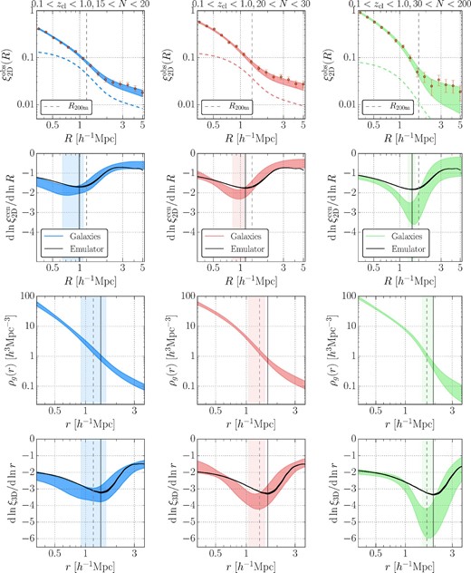
We show our projected cross-correlation function measurements and the model predictions from the MCMC chains in the first row of figures 1 and 2 for each cluster sample in table 1 with the fiducial absolute-magnitude cut Mz − 5log10h < −18.8 for galaxy selections. The second row shows constraints on the logarithmic derivative of the projected cross-correlation function based on our model fitting results. The third and fourth rows present constraints on the three-dimensional galaxy density profile and the logarithmic derivative of the three-dimensional profile, respectively. In the second and fourth rows, we also show the model predictions from the halo–matter cross-correlation function (i.e., dark matter distributions around clusters) in Nishimichi et al. (2019) and the mass–richness relation (Murata et al. 2019) presented in appendix 1 for comparisons.
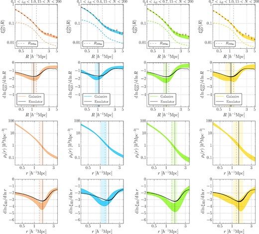
In the top row, we show observed projected cross-correlation measurements between the clusters and galaxies (points with error bars in red color) from left to right, for the Full, Low-z, Mid-z, and High-z cluster samples from table 3 with the fiducial absolute-magnitude cut Mz − 5log10h < −18.8 for galaxy selections. Shaded colored regions show the 16th and 84th percentiles of the model predictions from the MCMC chains for each cluster sample. The dashed profile curves in the top row show contributions from off-centered clusters to projected cross-correlation measurements at the best-fitting model parameters. The second row shows constraints on the logarithmic derivative of the projected cross-correlation profiles without off-centering effects in equation (7). The third row presents constraints on the three-dimensional galaxy density profile calculated as ρg(r) = 〈Σg〉ξ3D(r)/(2Rmax) (see subsection 3.1 for more details). The last row shows the constraints on the logarithmic derivative of the three-dimensional profiles. The vertical black dashed lines denote mean values of R200m shown in table 1 for the cluster samples. Black vertical shaded regions show model predictions from the halo–matter cross-correlation (i.e., dark matter distributions around clusters) and mass–richness relation in appendix 1 for |$R_{\rm sp}^{\rm 2D}$| in the second row and |$r_{\rm sp}^{\rm 3D}$| in the third and last rows from table 1, whereas colored vertical shaded regions show their constraints from the MCMC chains in each cluster sample. Black shaded profile regions in the second and last rows show derivative profiles from the model predictions for each cluster sample. (Color online)
In table 3, we show constraints on the model parameters and derived splashback features. The constraints on log10α, log10β, log10γ, fcen, and Roff parameters are determined mainly from the Gaussian priors, whereas those for the other parameters are well constrained by the measurements compared to their prior distributions. The χ2 values of the best-fitting model parameters in table 1 indicate that our fitting results are acceptable. Following Baxter et al. (2017), we list the values of the logarithmic derivative of the inner profiles [i.e., ρin(r)ftrans(r)] at the location of |$r_{\rm sp}^{\rm 3D}$| in table 1. These values are smaller than −3 with more than ∼2σ significance for all the samples. This result suggests that classical fitting functions like the Navarro–Frenk–White profiles (NFW; Navarro et al. 1996) have difficulty in fitting the observed cross-correlation measurements and provides the evidence of the splashback features (Baxter et al. 2017).
Model parameter constraints and derived constraints on splashback features with the fiducial absolute-magnitude cut.*
| Parameter | Full | Low-z | Mid-z | High-z | Low-N | Mid-N | High-N |
|---|---|---|---|---|---|---|---|
| log10ρs | |$1.97^{+0.58}_{-0.43}$| | |$1.31^{+0.63}_{-0.91}$| | |$1.83^{+0.68}_{-0.72}$| | |$2.10^{+0.56}_{-0.70}$| | |$2.13^{+0.55}_{-0.70}$| | |$1.28^{+0.64}_{-0.92}$| | |$1.87^{+0.71}_{-0.69}$| |
| log10α | |$-0.68^{+0.31}_{-0.36}$| | |$-0.75^{+0.54}_{-0.56}$| | |$-0.80^{+0.39}_{-0.50}$| | |$-0.73^{+0.30}_{-0.49}$| | |$-0.62^{+0.26}_{-0.46}$| | |$-0.71^{+0.52}_{-0.57}$| | |$-1.02^{+0.41}_{-0.46}$| |
| log10rs | |$-0.58^{+0.20}_{-0.27}$| | |$-0.21^{+0.58}_{-0.32}$| | |$-0.48^{+0.36}_{-0.32}$| | |$-0.64^{+0.32}_{-0.24}$| | |$-0.66^{+0.31}_{-0.23}$| | |$-0.22^{+0.60}_{-0.33}$| | |$-0.43^{+0.33}_{-0.34}$| |
| log10ρo | |$-0.48^{+0.14}_{-0.21}$| | |$-0.21^{+0.15}_{-0.24}$| | |$-0.75^{+0.31}_{-0.44}$| | |$-0.63^{+0.28}_{-0.47}$| | |$-0.44^{+0.17}_{-0.26}$| | |$-0.42^{+0.21}_{-0.36}$| | |$-0.74^{+0.44}_{-0.67}$| |
| S e | |$1.30^{+0.21}_{-0.26}$| | |$1.40^{+0.22}_{-0.29}$| | |$0.98^{+0.40}_{-0.48}$| | |$1.25^{+0.40}_{-0.54}$| | |$1.38^{+0.25}_{-0.33}$| | |$1.25^{+0.29}_{-0.43}$| | |$1.17^{+0.77}_{-0.64}$| |
| log10rt | |$0.16^{+0.11}_{-0.09}$| | |$0.02^{+0.18}_{-0.15}$| | |$0.13^{+0.16}_{-0.15}$| | |$0.16^{+0.20}_{-0.18}$| | |$0.16^{+0.29}_{-0.26}$| | |$0.01^{+0.21}_{-0.17}$| | |$0.13^{+0.07}_{-0.06}$| |
| log10β | |$0.77^{+0.22}_{-0.23}$| | |$0.72^{+0.19}_{-0.18}$| | |$0.70^{+0.21}_{-0.19}$| | |$0.78^{+0.22}_{-0.23}$| | |$0.73^{+0.22}_{-0.22}$| | |$0.72^{+0.20}_{-0.18}$| | |$0.81^{+0.19}_{-0.18}$| |
| log10γ | |$0.64^{+0.19}_{-0.20}$| | |$0.56^{+0.20}_{-0.19}$| | |$0.58^{+0.20}_{-0.19}$| | |$0.61^{+0.20}_{-0.20}$| | |$0.58^{+0.20}_{-0.20}$| | |$0.54^{+0.20}_{-0.18}$| | |$0.67^{+0.18}_{-0.18}$| |
| f cen | |$0.65^{+0.06}_{-0.06}$| | |$0.69^{+0.08}_{-0.08}$| | |$0.64^{+0.06}_{-0.06}$| | |$0.59^{+0.11}_{-0.12}$| | |$0.53^{+0.08}_{-0.08}$| | |$0.66^{+0.06}_{-0.06}$| | |$0.85^{+0.06}_{-0.06}$| |
| R off | |$0.56^{+0.07}_{-0.08}$| | |$0.40^{+0.09}_{-0.09}$| | |$0.56^{+0.08}_{-0.09}$| | |$0.61^{+0.08}_{-0.10}$| | |$0.59^{+0.06}_{-0.06}$| | |$0.53^{+0.09}_{-0.09}$| | |$0.55^{+0.10}_{-0.10}$| |
| |$r_{\rm sp}^{\rm 3D}\ [h^{-1}\:\mbox{Mpc}]$| | |$1.51^{+0.19}_{-0.18}$| | |$1.24^{+0.21}_{-0.19}$| | |$1.58^{+0.28}_{-0.25}$| | |$1.52^{+0.31}_{-0.45}$| | |$1.23^{+0.35}_{-0.33}$| | |$1.26^{+0.25}_{-0.21}$| | |$1.68^{+0.25}_{-0.19}$| |
| |$\frac{ {d}\ln \xi _{\rm 3D} }{ {d}\ln r }|_{r=r_{\rm sp}^{\rm 3D}}$| | |$-4.04^{+0.44}_{-0.65}$| | |$-3.69^{+0.34}_{-0.46}$| | |$-4.29^{+0.55}_{-0.75}$| | |$-4.12^{+0.63}_{-0.93}$| | |$-3.59^{+0.40}_{-0.58}$| | |$-3.89^{+0.41}_{-0.56}$| | |$-5.18^{+0.79}_{-1.13}$| |
| |$\frac{ {d}\ln (\rho _{\rm in} f_{\rm trans}) }{ {d}\ln r }|_{r=r_{\rm sp}^{\rm 3D}}$| | |$-5.51^{+0.95}_{-1.25}$| | |$-4.83^{+0.73}_{-0.92}$| | |$-5.28^{+0.85}_{-1.10}$| | |$-5.32^{+1.04}_{-1.38}$| | |$-4.70^{+0.80}_{-1.14}$| | |$-4.89^{+0.79}_{-1.01}$| | |$-6.24^{+1.04}_{-1.44}$| |
| |$\frac{ \rho _{\rm in}f_{\rm trans} }{ \rho _{\rm in}f_{\rm trans}+\rho _{\rm out} }|_{ r=r_{\rm sp}^{\rm 3D} }$| | |$0.66^{+0.11}_{-0.10}$| | |$0.67^{+0.13}_{-0.11}$| | |$0.78^{+0.10}_{-0.12}$| | |$0.73^{+0.12}_{-0.15}$| | |$0.68^{+0.12}_{-0.13}$| | |$0.74^{+0.13}_{-0.13}$| | |$0.81^{+0.10}_{-0.15}$| |
| |$R_{\rm sp}^{\rm 2D}\ [h^{-1}\:\mbox{Mpc}]$| | |$1.15^{+0.17}_{-0.18}$| | |$0.95^{+0.14}_{-0.12}$| | |$1.13^{+0.17}_{-0.15}$| | |$1.12^{+0.26}_{-0.36}$| | |$0.83^{+0.26}_{-0.19}$| | |$0.95^{+0.14}_{-0.13}$| | |$1.36^{+0.14}_{-0.12}$| |
| |$\frac{ {d}\ln \xi _{\rm 2D} }{ {d}\ln R }|_{R=R_{\rm sp}^{\rm 2D}}$| | |$-2.10^{+0.17}_{-0.22}$| | |$-2.01^{+0.17}_{-0.21}$| | |$-2.28^{+0.25}_{-0.32}$| | |$-2.24^{+0.27}_{-0.40}$| | |$-1.97^{+0.20}_{-0.29}$| | |$-2.14^{+0.21}_{-0.26}$| | |$-2.97^{+0.42}_{-0.63}$| |
| S/N | 59.2 | 45.4 | 39.5 | 44.8 | 44.4 | 39.2 | 30.2 |
| 〈Σg〉 [h2 Mpc−2] | 76.8 | 60.8 | 73.4 | 84.0 | 77.2 | 77.3 | 75.4 |
| |$\chi _{\rm min}^2/{\rm dof}$| | 11.5/10 | 19.6/10 | 6.3/10 | 19.2/10 | 11.3/10 | 15.6/10 | 8.9/10 |
*We show the median and the 16th and 84th percentiles of the posterior distribution of the model parameters for each cluster sample in table 1 with the fiducial absolute-magnitude cut Mz − 5log10h < −18.8. We present the derived constraints from MCMC chains on splashback features for each cluster sample. S/N denotes the signal-to-noise ratio within the radial bins for the fitting analyses, and 〈Σg〉 value is the mean galaxy surface density of galaxies after the galaxy selection for each cluster sample (see section 2.4 for more details). We also show the minimum chi-square (|$\chi _{\rm min}^{2}$|) with the number of degrees of freedom (dof) in the bottom row. As the model parameters with informative Gaussian priors (α, β, γ, fcen, and Roff) are determined strongly by the priors in table 2, we do not include them as free parameters when calculating dof (i.e., dof = 10 = 15 − 5, where 15 is the total number of data points and 5 is the total number of model parameters without informative priors). In appendix 3 we show correlations among the parameters for the Full sample.
The 1σ precisions of our constraints on |$r_{\rm sp}^{\rm 3D}$| compared to the median values are approximately |$12\%$|, |$16\%$|, |$17\%$|, |$25\%$|, |$28\%$|, |$18\%$|, and |$13\%$| for the Full, Low-z, Mid-z, High-z, Low-N, Mid-N, and High-N selections, respectively, after marginalizing over the off-centering effects with the fiducial absolute magnitude galaxy cut. These constraints are consistent with the model predictions from the halo–matter cross-correlation function in appendix 1 within 0.5σ, 1.9σ, 0.2σ, 0.2σ, 0.5σ, 1.6σ, and 1.1σ levels for Full, Low-z, Mid-z, High-z, Low-N, Mid-N, and High-N, respectively, whereas our constraints are consistent with the |$20\%$| smaller model predictions (i.e., |$0.8 \times r_{\rm sp, model}^{\rm 3D}$|) within 1.2σ, 0.2σ, 1.0σ, 0.9σ, 0.3σ, 0.2σ, and 0.7σ levels. Given the larger error bars due to the smaller survey area, our constraints are consistent with both the model predictions and their |$20\%$| smaller values. However, we note that our constraints on |$r_{\rm sp}^{\rm 3D}$| for the Low-z sample at 0.1 < zcl < 0.4 are on the lower side than the model prediction at the level of 1.9σ, which is in line with the constraints in the literature (More et al. 2016; Baxter et al. 2017; Chang et al. 2018) with clusters selected by another optical cluster-finding algorithm redMaPPer. Further investigation is warranted given our larger error bars. We note that we compare constraints from only red galaxies with the model predictions again for the Low-z, Mid-z, and High-z cluster samples in subsection 4.3, as these constraints are more precise than those without separations of red and blue galaxies. Our constraints with the fiducial absolute magnitude galaxy cut in figures 1 and 2 suggest that the three-dimensional profiles are slightly steeper (i.e., smaller derivative values) around the splashback radius than the model predictions from dark matter. We discuss a possible origin for these results in subsections 4.2 by comparing constraints from different absolute magnitude galaxy cuts.
4.2 Splashback features from different absolute magnitude galaxy cuts
We employ the Low-z cluster sample to derive constraints on splashback features with different absolute magnitude galaxy cuts, as we can use fainter absolute-magnitude cuts for the galaxies with lower redshift clusters given a fixed apparent magnitude limit, and the constraint on |$r_{\rm sp}^{\rm 3D}$| for the Low-z sample is better among the cluster samples as shown in table 3 with the fiducial absolute-magnitude cut. Specifically, we shift the absolute-magnitude cuts by one or two magnitudes to both fainter and brighter sides with the z-band magnitude compared to the fiducial absolute-magnitude cut Mz − 5log10h < −18.8 in subsection 4.1. The faintest absolute-magnitude cut (Mz − 5log10h < −16.8) corresponds to an apparent z-band magnitude limit of 24.1 at zcl = 0.4, which is shallower than the apparent magnitude cut for the galaxy catalog.
We show these constraints on the model parameters and splashback features in table 4 after marginalizing over the off-centering effects. We present our projected cross-correlation function measurements for the Low-z sample with the different absolute magnitude galaxy cuts and the model predictions from the MCMC chains in the left-hand panel of figure 3. The measurements with fainter absolute-magnitude cuts have lower amplitudes, indicating that brighter galaxies are more strongly clustered around clusters than fainter galaxies. The right-hand panel in figure 3 shows constraints on the three-dimensional galaxy density profile from the MCMC chains. We also show histogram comparisons of the constraints on splashback features in figure 4. Figure 4 indicates that the constraints on |$R_{\rm sp}^{\rm 2D}$| and |$r_{\rm sp}^{\rm 3D}$| are robust against the different absolute-magnitude cuts within the error bars. Specifically, the 1σ precisions of the constraints on |$r_{\rm sp}^{\rm 3D}$| compared to the median values are |$13\%$|, |$15\%$|, |$16\%$|, |$20\%$|, and |$30\%$| from the brightest to the faintest absolute-magnitude cut including the fiducial cut, respectively. Within these error bars, we do not see any systematic trend consistent with dynamical friction effects (i.e., smaller values for brighter galaxies), which is not surprising given expectations (a |$\lesssim 20\%$| shift of |$r_{\rm sp}^{\rm 3D}$| for our brightest galaxy sample and |${\lesssim}5\%$| shifts for other galaxy samples) from subhalos in simulations (More et al. 2016; Chang et al. 2018) with simplistic abundance matching methods. Note that the constraints on |$r_{\rm sp}^{\rm 3D}$| are preferred to be smaller than that predicted by the model across the five absolute magnitude range within these error bars, although moderate correlations exist among these constraints. Indeed, we confirm that there are moderate positive correlations in the jackknife cross-covariance for the projected cross-correlation measurements among these different magnitude cuts. Further investigation with reduced error bars from a larger survey area is warranted to constrain dynamical friction effects at an |$\sim 5\%$| level for the CAMIRA clusters.
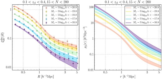
We show the results from table 4 with the Low-z cluster sample and the different absolute-magnitude cuts for galaxy selections after marginalizing over the off-centering effects. The left-hand panel shows the projected cross-correlation measurements and the 16th and 84th percentiles of the model predictions from the MCMC chains for each selection. The right-hand panel presents constraints on the three-dimensional galaxy density profile ρg(r) = 〈Σg〉ξ3D(r)/(2Rmax) (see subsection 3.1 for more details) from the MCMC chains for each selection. (Color online)
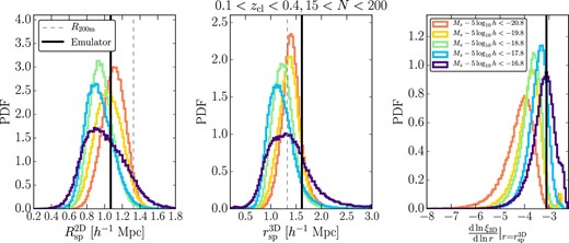
We show the probability distribution functions of splashback features from the MCMC chains for the analyses with the Low-z cluster sample and the different absolute-magnitude cuts for galaxy selections in table 4 and figure 3. The vertical black lines denote the model predictions from the halo–matter cross-correlation emulator and mass–richness relation in appendix 1 for comparisons. The vertical dashed lines show the mean value of R200m. (Color online)
Same as table 3, but for the Low-z cluster sample with different absolute-magnitude cuts for galaxy selections.*
| Low-z | Low-z | Low-z | Low-z | |
|---|---|---|---|---|
| Parameter | Mz − 5log10h < −20.8 | Mz − 5log10h < −19.8 | Mz − 5log10h < −17.8 | Mz − 5log10h < −16.8 |
| log10ρs | |$1.58^{+0.66}_{-0.92}$| | |$1.90^{+0.73}_{-0.86}$| | |$1.19^{+0.75}_{-0.97}$| | |$1.27^{+0.77}_{-1.22}$| |
| log10α | |$-0.82^{+0.57}_{-0.55}$| | |$-0.82^{+0.45}_{-0.52}$| | |$-0.80^{+0.50}_{-0.55}$| | |$-0.79^{+0.42}_{-0.53}$| |
| log10rs | |$-0.21^{+0.52}_{-0.33}$| | |$-0.43^{+0.44}_{-0.34}$| | |$-0.28^{+0.59}_{-0.36}$| | |$-0.44^{+0.54}_{-0.35}$| |
| log10ρo | |$-0.06^{+0.18}_{-0.27}$| | |$-0.09^{+0.15}_{-0.22}$| | |$-0.26^{+0.16}_{-0.26}$| | |$-0.43^{+0.24}_{-0.42}$| |
| S e | |$1.28^{+0.26}_{-0.33}$| | |$1.36^{+0.22}_{-0.27}$| | |$1.60^{+0.27}_{-0.35}$| | |$1.59^{+0.47}_{-0.53}$| |
| log10rt | |$0.08^{+0.12}_{-0.12}$| | |$0.10^{+0.14}_{-0.13}$| | |$0.01^{+0.21}_{-0.15}$| | |$0.12^{+0.29}_{-0.22}$| |
| log10β | |$0.76^{+0.20}_{-0.19}$| | |$0.73^{+0.20}_{-0.19}$| | |$0.72^{+0.20}_{-0.19}$| | |$0.72^{+0.21}_{-0.20}$| |
| log10γ | |$0.63^{+0.20}_{-0.20}$| | |$0.60^{+0.20}_{-0.20}$| | |$0.56^{+0.20}_{-0.19}$| | |$0.56^{+0.21}_{-0.20}$| |
| f cen | |$0.69^{+0.08}_{-0.08}$| | |$0.70^{+0.08}_{-0.08}$| | |$0.69^{+0.08}_{-0.08}$| | |$0.70^{+0.08}_{-0.08}$| |
| R off | |$0.39^{+0.08}_{-0.09}$| | |$0.40^{+0.09}_{-0.10}$| | |$0.39^{+0.09}_{-0.09}$| | |$0.39^{+0.09}_{-0.09}$| |
| |$r_{\rm sp}^{\rm 3D}\ [h^{-1}\:\mbox{Mpc}]$| | |$1.41^{+0.19}_{-0.17}$| | |$1.36^{+0.20}_{-0.20}$| | |$1.18^{+0.27}_{-0.21}$| | |$1.32^{+0.43}_{-0.36}$| |
| |$\frac{ {d}\ln \xi _{\rm 3D} }{ {d}\ln r }|_{r=r_{\rm sp}^{\rm 3D}}$| | |$-4.14^{+0.46}_{-0.68}$| | |$-3.77^{+0.37}_{-0.53}$| | |$-3.40^{+0.32}_{-0.43}$| | |$-3.20^{+0.41}_{-0.51}$| |
| |$\frac{ {d}\ln (\rho _{\rm in} f_{\rm trans}) }{ {d}\ln r }|_{r=r_{\rm sp}^{\rm 3D}}$| | |$-5.40^{+0.90}_{-1.23}$| | |$-5.03^{+0.79}_{-1.11}$| | |$-4.67^{+0.73}_{-0.93}$| | |$-4.55^{+0.76}_{-1.01}$| |
| |$\frac{ \rho _{\rm in}f_{\rm trans} }{ \rho _{\rm in}f_{\rm trans}+\rho _{\rm out} }|_{ r=r_{\rm sp}^{\rm 3D} }$| | |$0.71^{+0.12}_{-0.11}$| | |$0.66^{+0.12}_{-0.11}$| | |$0.60^{+0.16}_{-0.14}$| | |$0.56^{+0.20}_{-0.23}$| |
| |$R_{\rm sp}^{\rm 2D}\ [h^{-1}\:\mbox{Mpc}]$| | |$1.11^{+0.13}_{-0.14}$| | |$1.04^{+0.16}_{-0.15}$| | |$0.93^{+0.17}_{-0.14}$| | |$0.98^{+0.26}_{-0.21}$| |
| |$\frac{ {d}\ln \xi _{\rm 2D} }{ {d}\ln R }|_{R=R_{\rm sp}^{\rm 2D}}$| | |$-2.22^{+0.19}_{-0.24}$| | |$-2.01^{+0.16}_{-0.19}$| | |$-1.88^{+0.17}_{-0.21}$| | |$-1.73^{+0.18}_{-0.22}$| |
| S/N | 40.7 | 44.4 | 38.1 | 35.8 |
| 〈Σg〉 [h2 Mpc−2] | 8.4 | 24.2 | 139.5 | 300.0 |
| |$\chi _{\rm min}^2/{\rm dof}$| | 18.1/10 | 15.2/10 | 17.7/10 | 13.2/10 |
On the other hand, the logarithmic derivatives of the three-dimensional profiles at |$r_{\rm sp}^{\rm 3D}$| are larger for fainter absolute-magnitude cuts, as shown in the right-hand panel of figure 3 and figure 4. More et al. (2016) shows larger logarithmic derivative values at |$r_{\rm sp}^{\rm 3D}$| with decreasing maximum circular velocities of subhalos in simulations, which is consistent with our results. We expect that these differences in the derivative values are mainly caused by different ratios between the inner and outer material number densities (=ρinftrans/ρout) around the splashback radii, as splashback radii mark a halo boundary between the multi-stream and single-stream regions. We thus expect that derivative values would be smaller (i.e., steeper profiles) when the ratios are large at |$r_{\rm sp}^{\rm 3D}$|, whereas these values should be larger (i.e., shallower profiles) when the ratios are smaller. We confirm this expectation by checking that constraints on ρinftrans/(ρinftrans + ρout) = [1 + (ρinftrans/ρout)−1]−1 at |$r_{\rm sp}^{\rm 3D}$| for the fainter galaxy samples are systematically smaller than those for the brighter galaxy samples as presented in tables 3 and 4 although the error bars are not very small. Note that this correlation between the density ratios and the logarithmic derivative values at |$r_{\rm sp}^{\rm 3D}$| also exists in table 3 for the fiducial absolute-magnitude cuts and in table 5 for the color cuts presented in subsection 4.3.
Same as table 3, but for analyses with separations of red and blue galaxies.*
| Low-z | Low-z | Mid-z | Mid-z | High-z | High-z | |
|---|---|---|---|---|---|---|
| Parameter | red | blue | red | blue | red | blue |
| log10ρs | |$2.14^{+0.72}_{-0.82}$| | |$0.75^{+1.13}_{-1.68}$| | |$2.67^{+0.54}_{-0.58}$| | |$0.78^{+0.73}_{-0.87}$| | |$2.30^{+0.68}_{-0.68}$| | |$1.00^{+1.05}_{-1.57}$| |
| log10α | |$-0.91^{+0.44}_{-0.51}$| | |$-0.76^{+0.54}_{-0.53}$| | |$-0.75^{+0.28}_{-0.36}$| | |$-0.92^{+0.52}_{-0.52}$| | |$-0.80^{+0.38}_{-0.50}$| | |$-0.77^{+0.49}_{-0.55}$| |
| log10rs | |$-0.44^{+0.38}_{-0.34}$| | |$-0.35^{+0.60}_{-0.44}$| | |$-0.64^{+0.25}_{-0.24}$| | |$-0.14^{+0.48}_{-0.38}$| | |$-0.53^{+0.30}_{-0.31}$| | |$-0.45^{+0.60}_{-0.38}$| |
| log10ρo | |$-0.14^{+0.18}_{-0.26}$| | |$0.10^{+0.11}_{-0.30}$| | |$-0.80^{+0.37}_{-0.37}$| | |$-0.82^{+0.39}_{-0.45}$| | |$-0.55^{+0.33}_{-0.46}$| | |$-0.32^{+0.21}_{-0.32}$| |
| S e | |$1.24^{+0.24}_{-0.31}$| | |$1.78^{+0.27}_{-0.44}$| | |$0.68^{+0.44}_{-0.38}$| | |$0.85^{+0.49}_{-0.48}$| | |$0.98^{+0.42}_{-0.50}$| | |$1.55^{+0.49}_{-0.44}$| |
| log10rt | |$0.09^{+0.10}_{-0.09}$| | |$0.10^{+0.41}_{-0.25}$| | |$0.14^{+0.10}_{-0.09}$| | |$0.19^{+0.14}_{-0.12}$| | |$0.16^{+0.09}_{-0.13}$| | |$0.11^{+0.34}_{-0.23}$| |
| log10β | |$0.77^{+0.18}_{-0.17}$| | |$0.77^{+0.20}_{-0.20}$| | |$0.77^{+0.19}_{-0.19}$| | |$0.78^{+0.20}_{-0.19}$| | |$0.78^{+0.20}_{-0.20}$| | |$0.76^{+0.21}_{-0.21}$| |
| log10γ | |$0.66^{+0.19}_{-0.18}$| | |$0.59^{+0.20}_{-0.20}$| | |$0.67^{+0.18}_{-0.18}$| | |$0.61^{+0.20}_{-0.20}$| | |$0.67^{+0.19}_{-0.19}$| | |$0.60^{+0.20}_{-0.20}$| |
| f cen | |$0.70^{+0.08}_{-0.09}$| | |$0.70^{+0.08}_{-0.08}$| | |$0.64^{+0.06}_{-0.06}$| | |$0.64^{+0.06}_{-0.06}$| | |$0.59^{+0.11}_{-0.13}$| | |$0.61^{+0.10}_{-0.10}$| |
| R off | |$0.41^{+0.09}_{-0.10}$| | |$0.37^{+0.09}_{-0.08}$| | |$0.56^{+0.07}_{-0.07}$| | |$0.56^{+0.10}_{-0.10}$| | |$0.58^{+0.08}_{-0.17}$| | |$0.54^{+0.13}_{-0.14}$| |
| |$r_{\rm sp}^{\rm 3D}\ [h^{-1}\:\mbox{Mpc}]$| | |$1.45^{+0.17}_{-0.16}$| | |$1.05^{+0.63}_{-0.33}$| | |$1.72^{+0.22}_{-0.21}$| | |$1.76^{+0.36}_{-0.31}$| | |$1.72^{+0.24}_{-0.31}$| | |$1.15^{+0.45}_{-0.45}$| |
| |$\frac{ {d}\ln \xi _{\rm 3D} }{ {d}\ln r }|_{r=r_{\rm sp}^{\rm 3D}}$| | |$-4.55^{+0.53}_{-0.69}$| | |$-2.47^{+0.35}_{-0.47}$| | |$-5.62^{+0.79}_{-1.04}$| | |$-3.88^{+0.69}_{-0.93}$| | |$-5.13^{+0.76}_{-1.05}$| | |$-2.93^{+0.60}_{-0.77}$| |
| |$\frac{ {d}\ln (\rho _{\rm in} f_{\rm trans} ) }{ {d}\ln r }|_{r=r_{\rm sp}^{\rm 3D}}$| | |$-5.76^{+0.88}_{-1.13}$| | |$-4.28^{+0.86}_{-1.07}$| | |$-6.51^{+1.02}_{-1.35}$| | |$-5.10^{+0.92}_{-1.24}$| | |$-6.22^{+1.06}_{-1.42}$| | |$-4.53^{+0.90}_{-1.29}$| |
| |$\frac{ \rho _{\rm in}f_{\rm trans} }{ \rho _{\rm in}f_{\rm trans}+\rho _{\rm out} }|_{ r=r_{\rm sp}^{\rm 3D} }$| | |$0.74^{+0.10}_{-0.09}$| | |$0.31^{+0.25}_{-0.30}$| | |$0.86^{+0.06}_{-0.09}$| | |$0.73^{+0.12}_{-0.17}$| | |$0.81^{+0.09}_{-0.12}$| | |$0.50^{+0.21}_{-0.36}$| |
| |$R_{\rm sp}^{\rm 2D}\ [h^{-1}\:\mbox{Mpc}]$| | |$1.15^{+0.11}_{-0.12}$| | |$0.82^{+0.33}_{-0.23}$| | |$1.29^{+0.14}_{-0.12}$| | |$1.31^{+0.22}_{-0.22}$| | |$1.33^{+0.19}_{-0.26}$| | |$0.85^{+0.33}_{-0.30}$| |
| |$\frac{ {d}\ln \xi _{\rm 2D} }{ {d}\ln R }|_{R=R_{\rm sp}^{\rm 2D}}$| | |$-2.50^{+0.24}_{-0.28}$| | |$-1.27^{+0.13}_{-0.18}$| | |$-3.05^{+0.35}_{-0.42}$| | |$-1.72^{+0.25}_{-0.32}$| | |$-2.84^{+0.33}_{-0.41}$| | |$-1.47^{+0.21}_{-0.30}$| |
| S/N | 43.9 | 23.6 | 42.3 | 20.9 | 52.6 | 19.5 |
| 〈Σg〉 [h2 Mpc−2] | 14.4 | 21.1 | 13.6 | 33.3 | 15.6 | 38.4 |
| |$\chi _{\rm min}^2/{\rm dof}$| | 12.2/10 | 19.9/10 | 12.1/10 | 5.3/10 | 15.0/10 | 19.4/10 |
In particular, figure 4 shows that the constraint on the logarithmic derivative at |$r_{\rm sp}^{\rm 3D}$| from the faintest absolute-magnitude cut is consistent with the model prediction from the dark matter distribution, suggesting that the ratio between the inner and outer materials for the faintest galaxies should be on average similar to the one for the dark matter distribution around splashback radii for the Low-z cluster sample. Also, our results might indicate that a larger fraction of fainter galaxies accrete into cluster regions (|$r \lesssim r_{\rm sp}^{\rm 3D}$|) compared to brighter galaxies at 0.1 < zcl < 0.4, or that fainter galaxies have been selectively destroyed or merged compared to brighter galaxies to decrease number densities after infalls into cluster regions. We note that the blue fraction is higher at fainter magnitudes, thus the interpretation is also related to the results of subsection 4.3, although the absolute magnitude limits are not the same. It might be informative to compare these results with hydrodynamical simulations to constrain galaxy formation and evolution, possibly including relations between subhalo masses and galaxy luminosities.
4.3 Splashback features from red and blue galaxies
We employ a method from Nishizawa et al. (2018) to define red (quenched) and blue (star-forming) galaxy populations for each cluster redshift bin with the help of red-sequence measurements from the CAMIRA red member galaxy catalog described in subsection 2.2, without resorting to photometric redshifts of individual galaxies. This method uses a color–magnitude diagram for the CAMIRA member galaxies to derive a linear red-sequence relation at each cluster redshift within the redshift interval Δzcl = 0.05 (see subsection 2.4), where we employ g–r, r–i, and i–y color for clusters at 0.1 < zcl < 0.4, 0.4 < zcl < 0.7, and 0.7 < zcl < 1.0, respectively, and we use the z-band magnitude. These color combinations are chosen to be sensitive to the 4000 Å break from red galaxies at each redshift range. This method defines red galaxies with colors above a linear color–magnitude relation, which is 2σ lower (bluer) than the derived linear red-sequence mean relation at each cluster redshift bin and as a function of the z-band magnitude. We calculate these σ error values by averaging over the absolute magnitude limit for each cluster redshift bin, and these errors include the photometric errors as well as the intrinsic errors in the red sequence. With this method, we can define red and blue galaxy populations even outside the aperture size of the CAMIRA finder (R ≃ 1 h−1 Mpc in physical coordinates). Nishizawa et al. (2018) showed that number ratios between correlated red and blue galaxy populations around clusters marginally change by ∼0.1 at the filter transitions for the color combinations (i.e., zcl = 0.4, 0.7) at R < 1h−1 Mpc. We have confirmed that a difference of these selection criteria with the PDR2 is negligibly small from those in Nishizawa et al. (2018) with the first-year HSC data. In our analysis, we use the galaxy catalog after the same selection for the CAMIRA member catalog with |$\tt {z\_cmodel\_mag - a\_z}<24.0$| and |$\tt {z\_cmodel\_magsigma}<0.1$|, and we employ the absolute-magnitude cut Mz − 5log10h < −19.3 as described in subsection 2.3.
We note that this method is different from those in the literature. Specifically, Baxter et al. (2017) and Shin et al. (2019) employed photometric redshifts of individual galaxies to select galaxies for deriving color–magnitude diagrams as a function of redshift and to infer red/blue separation criteria based on percentile ranges in color values. On the other hand, Zürcher and More (2019) inferred g–r color cuts to separate red from blue galaxy population as a function of redshift with spectroscopic samples, although these spectroscopic samples are quite shallow and thus consist of galaxies that are brighter than their galaxies for cross-correlation measurements.
In figure 5 and table 5, we show the projected cross-correlation measurements and derived constraints. Consistently with the literature (Baxter et al. 2017; Nishizawa et al. 2018; Shin et al. 2019; Zürcher & More 2019), we find that red galaxies are more concentrated around cluster centers than blue galaxies in the projected measurements. We detect splashback features for both the red and blue galaxy populations defined by our selection criteria over 0.1 < zcl < 1.0, although the significances from the derivative of the inner profiles (Baxter et al. 2017) are smaller for blue galaxy populations of the Low-z and High-z cluster samples (∼1.5σ). Within the error bars, the constraints on |$r_{\rm sp}^{\rm 3D}$| are consistent among those for the fiducial absolute-magnitude cuts without the red and blue separation in subsection 4.1 and those for the red and blue galaxy populations at each redshift range. Due to their sharper profiles around |$r_{\rm sp}^{\rm 3D}$| (i.e., smaller derivative values), constraints on |$r_{\rm sp}^{\rm 3D}$| for only the red galaxies are more precise than those without the red and blue separation in subsection 4.1. Specifically, the 1σ precisions of the constraints on |$r_{\rm sp}^{\rm 3D}$| are approximately |$11\%$|, |$13\%$|, and |$16\%$| for the Low-z, Mid-z, and High-z cluster samples, respectively, when employing only the red galaxies, which are more precise than those in subsection 4.1 by |$\sim\! 10\%$| for the High-z cluster sample. These more precise constraints are consistent with the model predictions in table 1 within 1.0σ, 0.4σ, and 1.0σ levels, whereas these constraints are consistent with the |$20\%$| smaller model predictions within 1.0σ, 1.9σ, and 2.0σ levels for the Low-z, Mid-z, and High-z samples, respectively. We note that the constraints for the Mid-z and High-z cluster samples are more consistent with the model predictions (≲1σ levels) than the |$20\%$| smaller values of the model predictions (∼2σ levels). We also note that these analyses with the red galaxy populations approximately correspond to simulation results in Adhikari, Dalal, and Chamberlain (2014), which selectively uses simulation particles orbiting within clusters. They find that using simulation particles with small radial motions, which corresponds to preferentially selecting simulation particles within clusters, does not significantly bias the splashback radius measurement within the level of |$\sim 5\%$|–|$10\%$|. Also, based on the analysis of N-body simulations, Shin et al. (2019) argue that the splashback radius depends on the accretion time (that may correlate with the galaxy colors) of the subhalos used to measure it, although the dependence appears to be weak except for subhalos accreted very recently. Given our larger error bars from the limited area, further investigations are warranted to constrain |$r_{\rm sp}^{\rm 3D}$| values at the higher redshift ranges (0.4 < zcl < 1.0) more precisely with upcoming datasets.

Same as figure 1, but for the analyses with separations of red (red color) and blue (blue color) galaxies and an absolute-magnitude cut Mz − 5log10h < −19.3 for galaxy selections in subsection 4.3 and table 5 for the Low-z, Mid-z, and High-z cluster samples after marginalizing over the off-centering effects. (Color online)
We expect that the density profiles of blue galaxies would be consistent with a pure power-law without any splashback features when these blue galaxies are still on their first infall passage (Baxter et al. 2017; Shin et al. 2019; Zürcher & More 2019). We thus employ a pure power-law model that only marginalizes over the off-centering effects in analyses for blue galaxies, instead of the DK14 model for the three-dimensional profile, to check whether the power-law model can have reasonable |$\chi _{\rm min}^2$| values or not. We find that these analyses result in |$\chi ^{2}_{\rm min}/{\rm dof}=29.2/13, 21.7/13, 31.9/13$| for the Low-z, Mid-z, and High-z cluster samples, respectively. Their low p-values suggest that the DK14 model (table 5) can fit the measurements better than the power-law model given the difference in the minimum χ2 and the degree-of-freedom values over 0.1 < zcl < 1.0 (i.e., |$\Delta \chi ^{2}_{\rm min} \gtrsim 10$| by adding the six parameters for the DK14 model with the Gaussian priors on three of them). Note that, as shown in figure 5, the logarithmic derivative of the three-dimensional profile at |$r=r_{\rm sp}^{\rm 3D}$| for the blue galaxy population at 0.4 < zcl < 0.7 is smaller than those at the other redshift bins at the level of ∼2σ, possibly due to the different combinations of filters used to define the blue galaxy populations in Nishizawa et al. (2018) as described above.
At the same time, we also expect red galaxies to scatter into the blue population, especially at fainter magnitudes and higher redshift due to larger photometric errors. We estimate the contamination fraction from the red to the blue galaxy population to be fred ≃ 0.025 because we employ the 2σ lower limit for the separation criteria in Nishizawa et al. (2018). Compared to Zürcher and More (2019), we employ the same galaxy selection for the cross-correlation measurements as the one to define the red/blue separation criteria over all the redshift range, in order to apply this contamination fraction more consistently for fainter galaxies at higher redshift. This contamination could potentially alter the cross-correlation measurements for the blue populations, causing the observed splashback feature in the blue population. We follow a method found in appendix C of Zürcher and More (2019) to assess such contamination. First, we assume a pure power-law function for the blue galaxies with Se = 1.5 and the best-fitting parameter value for log10ρo in table 5 at each redshift bin. We then calculate a weighted sum of this power-law profile and the DK14 model profile for the red galaxy population with the best-fitting parameters in table 5 with a contamination fraction from the red to the blue population at each redshift bin (i.e., ρg, blue + fredρg, red). We find that the |$2.5\%$| contamination fraction alters the logarithmic derivative of the three-dimensional profile around |$r_{\rm sp}^{\rm 3D}$| of the red population by 0.1–0.2, which is smaller than values needed to explain the observed profiles (≳ 0.5 differences in the logarithmic derivative of the three-dimensional profiles around |$r_{\rm sp}^{\rm 3D}$|) in figure 5. We would require |$10\%$|–|$20\%$| contamination fractions from the red to the blue galaxy population to be consistent with the observed profiles for the blue populations when we assume a pure power-law function before such contaminations.
From these results, consistently with Zürcher and More (2019) from the different selection method on the red and blue galaxy populations, we conclude that some fraction of blue galaxies stay blue even after reaching their first apocenters of orbits within host clusters (i.e., splashback radii for these clusters) from the presence of the splashback feature in the blue galaxy populations when we define the blue galaxy populations using the method in Nishizawa et al. (2018). We note that Shin et al. (2019) found that their bluest galaxy sample defined by their criteria is consistent with a pure power-law, which is consistent with their bluest galaxy sample being on their first infall into their cluster samples. We expect that the difference from our results might come from the difference of the selection criteria of red and blue galaxy populations, as also discussed in Zürcher and More (2019).
Also, we investigate how the constraints on three-dimensional galaxy density profiles of the red and blue galaxy populations change around the locations of |$r_{\rm sp}^{\rm 3D}$| more directly in figure 5, whereas Baxter et al. (2017) and Shin et al. (2019) showed that their red/blue fractions abruptly change around |$r_{\rm sp}^{\rm 3D}$| in their projected profiles. Figure 5 shows that the three-dimensional galaxy density fractions between the red and blue galaxy populations change rapidly around the model predictions of |$r_{\rm sp}^{\rm 3D}$| in table 1 for all the redshift bins and that the blue galaxy populations in our separation criteria dominate at the outskirts of clusters over 0.1 < zcl < 1.0 after the 15 < N < 200 selection. The constraints on three-dimensional galaxy densities in figure 5 do not evolve significantly within the error bars over 0.1 < zcl < 1.0 for both the red and blue galaxy populations around clusters when selected by 15 < N < 200, including concentrations for red galaxy populations, possibly due to our off-centering marginalization compared to Nishizawa et al. (2018). In particular, we find that the three-dimensional galaxy densities for the red and blue populations become the same value at |$r=1.63^{+0.24}_{-0.15}\, h^{-1}\:\mbox{Mpc}$|, |$1.50^{+0.29}_{-0.20}\, h^{-1}\:\mbox{Mpc}$|, and |$1.76^{+0.28}_{-0.31}\, h^{-1}\:\mbox{Mpc}$| for the Low-z, Mid-z, and High-z cluster sample, respectively, where we calculate these values from the MCMC chains for each analysis. We note that we ignore positive cross-covariances between the projected cross-correlation measurements for the red and blue galaxy populations at each redshift bin for simplicity, and thus our error bars on these radial values are conservatively larger than those with these positive cross-covariances. These constraints are consistent with the model predictions of |$r_{\rm sp}^{\rm 3D}$| in table 1 within these error bars (≲1σ level) for all the redshift bins.
Because the fraction of the blue galaxy population starts to dominate outward at |$r \simeq r_{\rm sp}^{\rm 3D}$| over all the redshift bins, we expect that the blue galaxy population consists of a larger fraction of the infalling materials around the splashback radius than the red galaxy population over 0.1 < zcl <1.0 on average. However, the three-dimensional galaxy density profiles per comoving volumes for the blue galaxy populations do not increase at |$r<r_{\rm sp}^{\rm 3D}$| within the error bars over 0.1 < zcl < 1.0 as shown in figure 5, although the blue galaxy populations should fall into the cluster regions (|$r<r_{\rm sp}^{\rm 3D}$|) more frequently than the red galaxy populations. These results suggest that cluster influences on infalling galaxies should increase when these galaxies enter cluster regions at |$r<r_{\rm sp}^{\rm 3D}$| due to the multi-steaming materials, potentially leading to stronger quenching effects on blue galaxies into red galaxies (e.g., Hamabata et al. 2019) or more frequent merger rates with other galaxies to reduce the number of the blue galaxies selectively at |$r<r_{\rm sp}^{\rm 3D}$| for the absolute-magnitude cut. Alternatively, these results would imply that the multi-streaming regions at |$r<r_{\rm sp}^{\rm 3D}$| mix infalling galaxies with older galaxies which were accreted a longer time ago to cause an abrupt increase in red galaxy fractions at splashback radii.
5 Discussion
In subsection 5.1, we present how the off-centering effects cause biases and additional errors for constraints on splashback features. In subsection 5.2, we discuss the robustness of our results on the projection effects by employing mock catalogs with simplified cluster finders (Busch & White 2017; Sunayama & More 2019) and an HOD model to populate galaxies with halos phenomenologically with matching the cluster abundance density and lensing profiles to observations approximately.
5.1 Biases and errors on splashback features from off-centering effects
We check how the off-centering effect causes biases and additional errors for the analysis of the splashback features with our prior distribution in table 2 from the stacked lensing measurements in Murata et al. (2019) for each cluster sample. For this purpose, we repeat analyses without marginalizing over the off-centering effects for the Low-z, Mid-z, and High-z cluster samples with the fiducial setups in subsection 4.1 and with only the red galaxy population in subsection 4.3. We note that the prior distributions on the off-centering for higher redshift clusters have larger uncertainties due to lower signal-to-noise ratios of the stacked lensing measurements presented in Murata et al. (2019). We conservatively use the prior distributions from the stacked lensing measurements rather than those from a comparison of CAMIRA centers with X-ray selected clusters presented in Oguri et al. (2018) because the number of X-ray selected clusters that were matched to CAMIRA clusters (∼50) is limited, especially for higher-redshift and lower-richness clusters.
We show constraints on the splashback features for the analyses without marginalizing over the off-centering effects in table 6. We also present constraints on the logarithmic derivative of the three-dimensional profile with and without the off-centering model for the Low-z cluster sample with smaller off-centering effects and the High-z cluster sample with larger off-centering effects in figure 6. These results show that the median values for |$r_{\rm sp}^{\rm 3D}$| in the constraints without the marginalization are biased to |$\sim 10\%$| higher values compared to the fiducial results in tables 3 and 5 with marginalizing over the off-centering effects (see also More et al. 2016; Baxter et al. 2017; Zürcher & More 2019). The widths of the 16th and 84th percentile region for |$r_{\rm sp}^{\rm 3D}$| after marginalizing over the off-centering effects increase by |$21\%$|, |$36\%$|, and |$105\%$| for the Low-z, Mid-z, and High-z cluster samples, respectively, with the fiducial absolute-magnitude cut only compared to the analyses without the marginalization. On the other hand, the widths increase by |$22\%$|, |$30\%$|, and |$62\%$| for the Low-z, Mid-z, and High-z cluster samples, respectively, when employing only the red galaxy populations, which is a smaller degradation compared to that for only the absolute-magnitude cut mainly because the steeper profiles (i.e., smaller derivative values) for the red galaxy population only determine |$r_{\rm sp}^{\rm 3D}$| better even with the off-centering model. Thus we obtain the tighter constraints on |$r_{\rm sp}^{\rm 3D}$| when employing only the red galaxy population, especially for the higher-redshift cluster samples in subsection 4.3. Figure 6 also shows that the larger uncertainties in the off-centering increase errors for the derivative profile at inner radii for the High-z cluster sample, whereas the difference between the two results for the Low-z sample is smaller due to the smaller uncertainty of the offset distribution for the prior distribution.
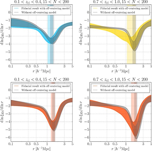
Top panels: We show how the off-centering effects change constraints on splashback features from tables 3 and 6 for the Low-z cluster sample with smaller off-centering effects and the High-z cluster sample with larger off-centering effects with the fiducial absolute-magnitude cut Mz − 5log10h < −18.8 for galaxy selections. We note that these fiducial results come from figure 1. Vertical shaded regions show the 16th and 84th percentiles of the model predictions on |$r_{\rm sp}^{\rm 3D}$| from the MCMC chains for each model, whereas shaded profile regions denote those on the logarithmical derivative profiles for the three-dimensional profile. Bottom panels: Same as the top panels, but for analyses with the red galaxy populations only and the absolute-magnitude cut Mz − 5log10h < −19.3 in tables 5 and 6. We also show these fiducial results in figure 5. (Color online)
Constraints on splashback features without marginalizing over off-centering effects.*
| Low-z | Mid-z | High-z | |||||
|---|---|---|---|---|---|---|---|
| Parameter | Full | Low-z | Mid-z | High-z | red | red | red |
| |$r_{\rm sp}^{\rm 3D}\ [h^{-1}\:\mbox{Mpc}]$| | |$1.63^{+0.12}_{-0.11}$| | |$1.37^{+0.17}_{-0.16}$| | |$1.76^{+0.21}_{-0.18}$| | |$1.68^{+0.21}_{-0.16}$| | |$1.52^{+0.14}_{-0.13}$| | |$1.86^{+0.17}_{-0.16}$| | |$1.87^{+0.18}_{-0.16}$| |
| |$\frac{ {d}\ln \xi _{\rm 3D} }{ {d}\ln r }|_{r=r_{\rm sp}^{\rm 3D}}$| | |$-4.29^{+0.40}_{-0.51}$| | |$-3.67^{+0.33}_{-0.44}$| | |$-4.44^{+0.53}_{-0.74}$| | |$-4.39^{+0.56}_{-0.72}$| | |$-4.68^{+0.50}_{-0.65}$| | |$-5.64^{+0.63}_{-0.83}$| | |$-5.38^{+0.69}_{-0.97}$| |
| |$\frac{ {d}\ln ( \rho _{\rm in}f_{\rm trans} ) }{ {d}\ln r }|_{r=r_{\rm sp}^{\rm 3D}}$| | |$-5.90^{+0.83}_{-1.06}$| | |$-4.97^{+0.82}_{-0.93}$| | |$-5.54^{+0.81}_{-1.10}$| | |$-5.82^{+0.99}_{-1.27}$| | |$-5.96^{+0.88}_{-1.11}$| | |$-6.52^{+0.92}_{-1.15}$| | |$-6.59^{+1.03}_{-1.35}$| |
| |$\frac{ \rho _{\rm in}f_{\rm trans} }{ \rho _{\rm in}f_{\rm trans}+\rho _{\rm out} }|_{ r=r_{\rm sp}^{\rm 3D} }$| | |$0.65^{+0.10}_{-0.10}$| | |$0.64^{+0.14}_{-0.11}$| | |$0.77^{+0.11}_{-0.12}$| | |$0.69^{+0.15}_{-0.15}$| | |$0.73^{+0.10}_{-0.09}$| | |$0.86^{+0.06}_{-0.09}$| | |$0.79^{+0.10}_{-0.11}$| |
| |$R_{\rm sp}^{\rm 2D}\ [h^{-1}\:\mbox{Mpc}]$| | |$1.36^{+0.08}_{-0.08}$| | |$1.07^{+0.11}_{-0.10}$| | |$1.37^{+0.10}_{-0.10}$| | |$1.42^{+0.11}_{-0.10}$| | |$1.24^{+0.09}_{-0.08}$| | |$1.46^{+0.08}_{-0.08}$| | |$1.53^{+0.09}_{-0.09}$| |
| |$\frac{ {d}\ln \xi _{\rm 2D} }{ {d}\ln R }|_{R=R_{\rm sp}^{\rm 2D}}$| | |$-2.18^{+0.15}_{-0.19}$| | |$-1.96^{+0.14}_{-0.16}$| | |$-2.27^{+0.21}_{-0.27}$| | |$-2.30^{+0.23}_{-0.29}$| | |$2.54^{+0.21}_{-0.25}$| | |$-3.09^{+0.25}_{-0.29}$| | |$-2.94^{+0.29}_{-0.37}$| |
| |$\chi _{\rm min}^2/{\rm dof}$| | 9.1/10 | 19.4/10 | 6.0/10 | 17.0/10 | 11.7/10 | 12.5/10 | 13.2/10 |
*We show the results without marginalizing over off-centering effects in the model fitting described in subsection 5.1. We use the fiducial absolute-magnitude cut Mz − 5log10h < −18.8 for galaxy selections in the constraints without red in the second row, whereas we employ the absolute-magnitude cut Mz − 5log10h < −19.3 and the red galaxy criteria in subsection 4.3 for the constraints with red. In subsection 5.1, we discuss biases and errors in the constraints from off-centering effects by comparing with the fiducial results after marginalizing over off-centering effects in tables 3 and 5.
Our result indicates that constraints on splashback features can be improved further by reducing the uncertainties of offset distributions, especially for clusters at higher redshifts. We note that upcoming datasets of lensing measurements with higher signal-to-noise ratios should reduce uncertainties of the off-centering that we adopt for the prior distribution, leading to tighter constraints on splashback features. We could instead use upcoming X-ray datasets for the high-redshift clusters to constrain offset distributions by checking offsets between X-ray and CAMIRA cluster centers for a large number of clusters.
5.2 Potential biases from projection effects
Optical cluster-finding algorithms such as CAMIRA and redMaPPer could preferentially detect clusters with filamentary structures along the line-of-sight as galaxies in the filament boosts observed richness. Such projection effects possibly cause some biases in a non-trivial way to observed splashback features based on the DK14 fitting in which the three-dimensional spherical symmetry is implicitly assumed, as the optical cluster selections are based on cluster richness values. Also, aperture sizes in optical cluster-finding algorithms could imprint some effects on the observed splashback features because cluster finders preferentially select clusters with higher galaxy density fluctuations within their aperture size, which is comparable to the scale of splashback features in projected space (Busch & White 2017; Chang et al. 2018; Sunayama & More 2019). We investigate possible projection effects with mock observations and simplified cluster-finding algorithms for CAMIRA and redMaPPer cluster-finding algorithms (hereafter CAMIRA-like and redMaPPer-like, respectively), partly following methods presented in Busch and White (2017) and Sunayama and More (2019), as detailed below.
For this purpose, we use a suite of cosmological N-body simulations generated by the Dark Quest campaign (Nishimichi et al. 2019) with a box size of 1 h−1 Gpc on a side and mass resolution of ≃ 1010 h−1 M⨀ for the Planck cosmology at z = 0.25 (see appendix 1 for more details). We select one realization of the simulations at z = 0.25 because this redshift is close to that for one of the most precise measurements in More et al. (2016) with the SDSS redMaPPer clusters, and projection effects are expected to be pronounced at lower redshift for a fixed cluster redshift error due to the larger non-linear structure growth. In particular, we employ halo catalogs based on Rockstar (Behroozi et al. 2013) to populate galaxies within halos, and dark matter to measure stacked lensing profiles around clusters to check an approximate consistency with the observation for the CAMIRA-like cluster finder (Murata et al. 2019) and the redMaPPer-like cluster finder (Murata et al. 2018).
Given the HOD galaxy catalog for cluster selections, we use a simplified mock cluster-finding algorithm for CAMIRA accounting for cluster member probabilities, following a methodology presented in Sunayama and More (2019) for redMaPPer. We employ a top-hat filter along the line-of-sight around each halo center in the simulation to select member galaxies and then estimate an optical richness for each cluster to mimic photometric redshift uncertainties in observations, following methods presented in Busch and White (2017) and Sunayama and More (2019), as our mock galaxies do not have realistic galaxy color information (i.e., we instead assume all the HOD galaxies are red-sequence galaxies used for cluster selections). We adopt an effective projection length of deff = 40 h−1 Mpc, based on a typical standard deviation of the differences between cluster redshift and spectroscopic redshift of BCGs (when available) for the HSC CAMIRA clusters (≡ Δzcl) through deff ≃ Δzcl/H(z), which is roughly a constant value over 0.1 ≤ zcl ≤ 1.0 within a precision of ∼5 h−1 Mpc around 40 h−1 Mpc. Note that we differentiate central and satellite galaxies in the mock galaxy catalog, and we only consider central galaxies as potential cluster centers (i.e., we ignore off-centering effects for simplicity).
We also employ the redMaPPer-like cluster-finding algorithm with the different HOD galaxy catalog. We refer to subsection 3.2 in Sunayama and More (2019) for more details on this algorithm, which is similar to that for the CAMIRA-like one above. One difference from Sunayama and More (2019) is that we use the projection length of deff = 40 h−1 Mpc following the CAMIRA-like algorithm. We only consider central galaxies as cluster centers, and we start our percolation by ranking central galaxies according to their halo masses, in descending order, to assign richness values in the first step, as described in Sunayama and More (2019). After the first richness assignments, we repeat the richness estimations a few times to converge, because the aperture size depends on richness values λ for redMaPPer,2 as Rc(λ) = 1.0 × (λ/100)0.2 h−1 Mpc in physical coordinates, where its spatial filter is based on the normalized projected NFW profile and an error function with a smooth truncation at R = Rc. Note that the aperture size of redMaPPer is smaller than that of CAMIRA at λ < 100. Furthermore, redMaPPer estimates and subtracts the background galaxy level in cluster selections assuming a constant value (i.e., a global value) in projected spaces, whereas CAMIRA does it locally to account for large-scale structure as described above. In order to investigate aperture-size effects on splashback features below, we also apply a redMaPPer-like algorithm with a larger aperture size of 1.35 × (λ/100)0.2 h−1 Mpc in physical coordinates. In this case, the aperture size at λ = 20 is comparable to that for CAMIRA.
For a consistency check on the setups of the HOD galaxy catalogs and the simplified cluster-finding algorithms, we investigate whether cluster abundance densities and lensing profiles from the dark matter around the clusters match approximately to the observations. For the CAMIRA-like cluster-finding algorithm, we employ the abundance measurements from the CAMIRA catalog based on PDR2 in subsection 2.2 at 0.1 < zcl < 0.4 with the corresponding survey volume, and the lensing measurements in Murata et al. (2019) for the Low-z cluster sample (0.1 < zcl < 0.4) in several richness bins. In figure 7, we show that the cluster abundance density from our mock catalog and simplified cluster-finder is larger than observations, but is consistent within a |$\sim 30\%$| level especially for a large number of low-richness clusters. We note that observed abundances in different richness bins are positively correlated especially at lower-richness bins (see figures 1 and 2 in Murata et al. 2019, for more details), and that these levels of matching is much better than those from the Millennium Simulation in Busch and White (2017) and Sunayama and More (2019), where their cluster abundance densities are ∼3 times larger than observations. The overestimation of cluster number is due to the different ways red galaxies could be populated. We also show in figure 7 that the lensing profiles from our mock catalog at 15 < N < 20, 20 < N < 30, and 30 < N < 200 reproduce the observed lensing profiles in Murata et al. (2019) for the Low-z cluster sample quite well within the error-bars in observations. They are also consistent with the best-fitting model in Murata et al. (2019) at a |$\sim 10\%$| level. In particular, a mean mass averaged over halos with identified central galaxies at 15 < N < 200 in the mock catalog for the CAMIRA-like finder is 1.8 × 10¹⁴ h−1 M⨀, which is consistent with the one in table 1 within the 1σ uncertainty for the Low-z cluster sample derived from the mass–richness relation in Murata et al. (2019). The total number of clusters in the simulation for the CAMIRA-like finder is 23486 at 15 < N < 200. For the redMaPPer-like cluster-finding algorithm with the fiducial aperture size, we also check for consistency with the observation of the SDSS redMaPPer at 0.1 < zcl < 0.33 in Murata et al. (2018). In figure 8 we show the comparison, suggesting that the cluster abundance density and lensing profiles for the redMaPPer-like cluster-finder also match the observation approximately.
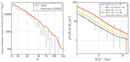
Consistency check for the CAMIRA-like cluster-finding algorithm in our mock catalog. Left-hand panel: We compare cluster abundance densities between the observation from the CAMIRA cluster catalog based on PDR2 used for this paper and the mock catalog. Error bars for the observation is based on the Poisson errors for simplicity. With the sample covariance contribution, the diagonal errors increase by ∼1.3 compared to the Poisson errors with a large positive correlation among different richness bins (see figures 1 and 2 in Murata et al. 2019, for more details). Note that the volume of the mock catalog is ∼20 times larger than that of the observation at 0.1 < zcl < 0.4. Right-hand panel: We compare lensing profiles from the observations at 0.1 < zcl < 0.4 in Murata et al. (2019) and our mock cluster catalog in three richness bins. Solid lines show the lensing profiles from the mock catalog. Dashed lines denote the model predictions at the best-fitting parameters in Murata et al. (2019), and points with error-bars are the observed lensing measurements from data. Note that there are large positive correlations of errors at larger radii, as shown in figure 2 of Murata et al. (2019), and that the model and data are affected by the off-centering effects at R ≲ 1.5 h−1 Mpc (Murata et al. 2019). (Color online)

Same as figure 7, but for the redMaPPer-like cluster-finding algorithm with the fiducial aperture size in our mock catalog. We use observational measurements of the abundance and lensing profiles for the SDSS redMaPPer clusters at 0.1 < zcl < 0.33 from Murata et al. (2018). We also use the best-fitting model for the lensing profiles from Murata et al. (2018) in the right-hand panel. (Color online)
Given the cluster catalog with halo mass and richness values and the HOD galaxy catalog, we conduct mock observations with the DK14 fitting and mock model calculations with the emulator by closely following our procedure in the data analysis with real data to investigate whether these two values match within statistical errors for each mock cluster-finding algorithm, or not due to the projection effects. First, we estimate the splashback radius in the three-dimensional space |$r_{\rm sp}^{\rm 3D}$| from the projected cross-correlation functions in the mock catalogs. We compute these projected cross-correlation functions for each cluster sample after selection and the HOD galaxy catalog, where we use the maximum integral scale along the line-of-sight of 100 h−1 Mpc. We use 64 jackknife regions in order to compute the covariance in these measurements. We then repeat the MCMC fitting procedure with the DK14 profile, assuming the spherical symmetry, as in subsection 3.1, to the mock projected cross-correlation functions in order to estimate |$r_{\rm sp}^{\rm 3D}(\equiv r_{\rm sp, DK14\ MCMC}^{\rm 3D})$|. Note that we do not include the off-centering model for simplicity, because our mock cluster-finding algorithms do not account for the off-centering effects. Secondly, we calculate the mock model calculations with the emulator following appendix 1. For each cluster sample after selection, we calculate the average profiles of ξhm(r; M, z) at z = 0.25 by stacking over the halo masses for massive main halos with identified central galaxies for each cluster sample, similarly to the approach in appendix 1 to calculate the splashback radius as model predictions |$(\equiv r_{\rm sp, emulator\ stack}^{\rm 3D})$|. These model predictions in the mock catalogs correspond to those for the real data with the observed mass–richness relation used in appendix 1, as long as the observed mean mass given a fixed richness value via the mass–richness relation from weak lensing measurements is sufficiently close to true masses of such massive main halos. As discussed in Shin et al. (2019), the location of a splashback radius scales as ∼M1/3 and thus we require roughly |$30\%$| biases in the observed mass–richness relation compared to the massive main halo masses to explain a |$10\%$| deviation in model predictions for |$r_{\rm sp}^{\rm 3D}$|, but this level of mass bias would be unlikely (Sunayama et al. 2020). Thus, our mock model predictions closely resemble the procedure for the real data in appendix 1. These procedures in the mock catalog are different from those in Sunayama and More (2019) which use the Millennium Simulation, where the Abel transformation is employed to evaluate the asymmetry of galaxies around clusters after richness selections in projected spaces. We instead investigate the biases in |$r_{\rm sp}^{\rm 3D}$| by following the procedures for the real data more directly.
We first show comparisons for cluster samples with mass threshold selections as M200m > Mmin. These selections are not related to richness values, and hence this comparison shows the difference between |$r_{\rm sp, DK14\ MCMC}^{\rm 3D}$| and |$r_{\rm sp, emulator\ stack}^{\rm 3D}$| for cases without projection effects. We expect that these values match quite well because we construct the HOD galaxy catalog based on ξhm(r; M, z) for the radial distribution of satellite galaxies in |$r<r_{\rm sp}^{\rm 3D}$| with a sharp drop at |$r=r_{\rm sp}^{\rm 3D}$|. For the HOD catalog with the CAMIRA-like finder, we find that |$r_{\rm sp, DK14\ MCMC}^{\rm 3D}/r_{\rm sp, emulator\ stack}^{\rm 3D} \simeq 1.05$| over a wide mass range above M200m = 1013 h−1 M⨀ as shown in the left-hand panel of figure 9. The values for |$r_{\rm sp, DK14\ MCMC}^{\rm 3D}$| are slightly larger than |$r_{\rm sp, emulator\ stack}^{\rm 3D}$| because our HOD model catalog employs α = 1.15 for the mass dependence in the number of HOD galaxies as |$\propto M_{\rm 200m}^{\alpha }$| with a larger weight on more massive halos, whereas the approximately corresponding number for the emulator stack is |$\int _{0}^{ r_{\rm sp}^{\rm 3D} } r^2 {d} r \xi _{\rm hm}(r; M_{\rm 200m}, z)$|, which is roughly propotional to M200m. For the different HOD catalog with the redMaPPer-like cluster finders, we find that |$r_{\rm sp, DK14\ MCMC}^{\rm 3D}/r_{\rm sp, emulator\ stack}^{\rm 3D} \simeq 1.01$| over the wide mass range in the left-hand panel of figure 10, as this HOD model catalog instead employs α = 1. We use |$r_{\rm sp, DK14\ MCMC}^{\rm 3D}/r_{\rm sp, emulator\ stack}^{\rm 3D} = 1.05$| or 1.01 for the CAMIRA-like and redMaPPer-like cluster finders, respectively, as a baseline when we discuss the significance of projection effects in comparisons between |$r_{\rm sp, DK14\ MCMC}^{\rm 3D}$| and |$r_{\rm sp, emulator\ stack}^{\rm 3D}$| below.
![Results for the CAMIRA-like cluster-finding algorithm in our mock catalog. Left-hand panel: Comparison of estimated locations of $r_{\rm sp}^{\rm 3D}$ based on the DK14 profile fitting assuming the spherical symmetry to the projected cross-correlation functions between halos and the HOD galaxies in the simulation, and those from the emulator stack when selecting halos based on halo masses (i.e., without projection effects related to richness values). As expected from the construction of the HOD galaxy catalog, the two values match quite well (see text for more details). The blue horizontal line denotes the average value of the ratio, 1.05. We estimate the error-bars from the MCMC chains with half widths of the $68\%$ percentile region. Right-hand panel: Similarly to the left-hand panel, we compare the observed splashback radii from the DK14 fitting to the projected cross-correlation functions with those from the emulator stack, but here we select halos based on richness values with projection effects. We use 10 richness bins with bin edges of N = [15.0,17.6,20.6,24.2,28.4,33.3,39.1,45.9,53.8,74.0,200.0]. The constraint for the CAMIRA-like finder is $r_{\rm sp, DK14\ MCMC}^{\rm 3D}/r_{\rm sp, emulator\ stack}^{\rm 3D} = 1.06 \pm 0.03$ for the sample of 15 < N < 200, which is consistent with 1.05 from the mass selection in the left-hand panel without projection effects, and its uncertainty is smaller than our statistical errors in the HSC data analysis. Note that we estimate this ratio by repeating the procedure for the cluster sample of 15 < N < 200. (Color online)](https://oup.silverchair-cdn.com/oup/backfile/Content_public/Journal/pasj/72/4/10.1093_pasj_psaa041/3/m_pasj_72_4_64_f13.jpeg?Expires=1749741408&Signature=p2g5kvhOgKSHFQKTmJ1xwHchh-h1md~Nj7~T0AaipGOjhST0rN2p2i1no~nhhhalZPbvipDTVDahUNhkhMqw0uPxAK0wvnOz1bT5c6Trmd~ZYap15Jk1jcMuGn0vsnsgWd8IBkJ43dxnoDQzy63pGL0DS8A8xYgEZkftwJLUlbgzTUX-xtxC7nW4olhzTgnq-yoyN1erlHRzJpJp7KCmz30hjk6cwNuSI8msH-R7XwS8eKWecsW7ICNKQrt7HwGCgpWr5LR9sMSxyC2raNFeE-Vp~LJJtfg8mJ9vXPCbEpVZjPGN0623X1~F7Qf~B8aJeDtIPtvLS3RRkg70q1zdIw__&Key-Pair-Id=APKAIE5G5CRDK6RD3PGA)
Results for the CAMIRA-like cluster-finding algorithm in our mock catalog. Left-hand panel: Comparison of estimated locations of |$r_{\rm sp}^{\rm 3D}$| based on the DK14 profile fitting assuming the spherical symmetry to the projected cross-correlation functions between halos and the HOD galaxies in the simulation, and those from the emulator stack when selecting halos based on halo masses (i.e., without projection effects related to richness values). As expected from the construction of the HOD galaxy catalog, the two values match quite well (see text for more details). The blue horizontal line denotes the average value of the ratio, 1.05. We estimate the error-bars from the MCMC chains with half widths of the |$68\%$| percentile region. Right-hand panel: Similarly to the left-hand panel, we compare the observed splashback radii from the DK14 fitting to the projected cross-correlation functions with those from the emulator stack, but here we select halos based on richness values with projection effects. We use 10 richness bins with bin edges of N = [15.0,17.6,20.6,24.2,28.4,33.3,39.1,45.9,53.8,74.0,200.0]. The constraint for the CAMIRA-like finder is |$r_{\rm sp, DK14\ MCMC}^{\rm 3D}/r_{\rm sp, emulator\ stack}^{\rm 3D} = 1.06 \pm 0.03$| for the sample of 15 < N < 200, which is consistent with 1.05 from the mass selection in the left-hand panel without projection effects, and its uncertainty is smaller than our statistical errors in the HSC data analysis. Note that we estimate this ratio by repeating the procedure for the cluster sample of 15 < N < 200. (Color online)
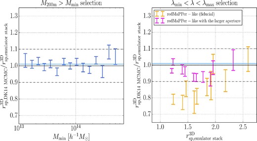
Same as figure 9, but for the redMaPPer-like cluster-finding algorithms with the fiducial and larger aperture sizes in our mock catalog. The blue horizontal line denotes the average value of the ratio in the left-hand panel, 1.01. We use the same richness bins as figure 9 in the right-hand panel. The constraint for the redMaPPer-like with the fiducial aperture size is |$r_{\rm sp, DK14\ MCMC}^{\rm 3D}/r_{\rm sp, emulator\ stack}^{\rm 3D} = 0.86 \pm 0.03$| for the sample of 20 < λ < 100, which is smaller than 1.01 from the mass cuts by |$\sim 15\%$| and is consistent with the trend of the smaller value in observation (More et al. 2016; Chang et al. 2018). The biases are smaller at higher richness bins, which is also consistent with the literature (Shin et al. 2019). Specifically, the constraints for the samples of 15 < λ < 40 and 40 < λ < 100 are |$r_{\rm sp, DK14\ MCMC}^{\rm 3D}/r_{\rm sp, emulator\ stack}^{\rm 3D} = 0.72 \pm 0.05$| and |$r_{\rm sp, DK14\ MCMC}^{\rm 3D}/r_{\rm sp, emulator\ stack}^{\rm 3D} = 0.91 \pm 0.04$|, respectively. In contrast, using the redMaPPer-like with the larger aperture (× 1.35), the biases are significantly reduced even at lower richness bins within a |$\sim 5\%$| level compared to the mass cuts. (Color online)
Next, we show comparisons when selecting the halos with richness values for each cluster-finding algorithm in the right-hand panels of figures 9 and 10 to investigate projection effects on the splashback radius. For the CAMIRA-like cluster-finding algorithm, we find that |$r_{\rm sp, DK14\ MCMC}^{\rm 3D}/r_{\rm sp, emulator\ stack}^{\rm 3D}$| is consistent with that (i.e., 1.05) without projection effects at all richness bins above N = 15 at a precision of |$5\%$|, which is well below our statistical errors. In particular, the constraint for the sample of 15 < N < 200 is |$r_{\rm sp, DK14\ MCMC}^{\rm 3D}/r_{\rm sp, emulator\ stack}^{\rm 3D} = 1.06 \pm 0.03$|, with |$r_{\rm sp, emulator\ stack}^{\rm 3D} = 1.6\:h^{-1}\:\mbox{Mpc}$|. This result suggests that the biases of projection effects on |$r_{\rm sp}^{\rm 3D}$| estimated from the DK14 fitting should be negligible for CAMIRA in our HSC data analysis. As CAMIRA employs the constant aperture size independent of richness values, our mock analysis confirms that we indeed detect the physical splashback radii of halos rather than artifacts due to optical cluster finding that selects overdensities of galaxies within a given radius.
In the right-hand panel of figure 10, we also show the results for the redMaPPer-like algorithms. For the redMaPPer-like finder with the fiducial aperture size, we find that the observed splashback radii from the DK14 fitting are smaller than the model predictions, especially at lower richness values. Specifically, the constraint for the sample of 20 < λ < 100 is |$r_{\rm sp, DK14\ MCMC}^{\rm 3D}/r_{\rm sp, emulator\ stack}^{\rm 3D} = 0.86 \pm 0.03$| with |$r_{\rm sp, emulator\ stack}^{\rm 3D} = 1.7\:h^{-1}\:\mbox{Mpc}$|, suggesting an |$\sim \!\! 15\%$| bias compared to that without projection effects (i.e., 1.01). This trend is consistent with the results of the smaller observed splashback radii in the literature with redMaPPer clusters (More et al. 2016; Chang et al. 2018; Shin et al. 2019). In particular, the mass scales for More et al. (2016) and Chang et al. (2018) are comparable to that for 20 < λ < 100 above, whereas the mass scale for Shin et al. (2019) is more massive with |$r_{\rm sp, model}^{\rm 3D} \simeq 2.1\:h^{-1}\:\mbox{Mpc}$|. As shown in figure 11, the result of Shin et al. (2019) is more consistent with their model prediction, which is also consistent with the right-hand panel of figure 10, with smaller biases at higher richness values.

Comparison of ratios between the observed |$r_{\rm sp}^{\rm 3D}$| and its model prediction for fiducial results among the literature with our results as a function of mean redshift in cluster samples. We refer to table 3 in Shin et al. (2019) as a summary table. Red error-bars show our results with the CAMIRA clusters from the red galaxy populations only in subsection 4.3 for the Low-z, Mid-z, and High-z cluster samples. We employ median values with errors calculated from a half width of the |$68\%$| percentile region in table 5 for simplicity. Orange error-bars show constraints with the redMaPPer clusters from SDSS (More et al. 2016) and DES (Chang et al. 2018; Shin et al. 2019), from low- to high-redshift values. The average mass scale for More et al. (2016) and Chang et al. (2018) is comparable to that for our constraints in red color, but the constraint in Shin et al. (2019) is based on a more massive mass scale with |$r_{\rm sp, model}^{\rm 3D}=1.60, 1.46, 2.07\, h^{-1}\:\mbox{Mpc}$| for these constraints, respectively. Blue error-bars denote constraints with clusters selected by the Sunyaev–Zel’dovich (SZ) effects in the Planck data (Zürcher & More 2019) and the South Pole Telescope data (Shin et al. 2019) from low- to high-redshift values. The horizontal dashed line shows the |$20\%$| smaller values compared to the model predictions, as suggested by the literature. (Color online)
In addition, we show that the biases are significantly reduced even at lower richness bins for the redMaPPer-like finder with the larger (× 1.35) aperture size as |$r_{\rm sp, DK14\ MCMC}^{\rm 3D}/r_{\rm sp, emulator\ stack}^{\rm 3D} \simeq 0.95$|. These results suggest that the smaller aperture size in the fiducial redMaPPer-like finder than the splashback feature scale of |$R_{\rm sp, model}^{\rm 2D}\simeq 1.1\:h^{-1}\:\mbox{Mpc}$| in comoving coordinates (see table 1) induces selection bias effects on the observed splashback radii. Specifically, the fiducial redMaPPer finder uses R = 0.72 h−1 Mpc at λ = 20 in physical coordinates (i.e., R = 0.90 h−1 Mpc in comoving coordinates at z = 0.25) which is smaller than the scale of |$R_{\rm sp, model}^{\rm 2D}$| above. On the other hand, the redMaPPer with the larger aperture at λ = 20 and CAMIRA with the smaller biases on the observed splashback radii employs R = 1.0 h−1 Mpc in physical coordinates (R = 1.25 h−1 Mpc in comoving coordinates at z = 0.25), which is larger than the scale of |$R_{\rm sp, model}^{\rm 2D}$|. The biases for the fiducial redMaPPer-like finder are reduced at larger richness values in figure 10, probably because its aperture size increases as ∝ λ0.2 with |$R = R_{\rm sp, model}^{\rm 2D}$| around λ = 50 at z = 0.25. However, |$r_{\rm sp, DK14\ MCMC}^{\rm 3D}/r_{\rm sp, emulator\ stack}^{\rm 3D}$| for the redMaPPer-like finder with the larger aperture is smaller than those for the mass cuts by a |$\sim 5\%$| level, which could be due to the difference between their radial filters. In particular, the CAMIRA finder employs the local background subtraction in richness estimations to account for large-scale structure contributions, which might provide another reason for the smaller projection effects on splashback radii.
It is important to confirm these results with more realistic mock galaxy populations with galaxy colors by applying more realistic cluster-finding algorithms for them when available, as here we empirically employ the HOD model and the simplified cluster-finding algorithms. Nevertheless, our results are informative to clarify the different effects of CAMIRA and redMaPPer on splashback radii at least qualitatively. It is also interesting to compare splashback features for these two cluster-finding algorithms directly by using the same datasets for clusters, galaxies, and weak lensing calibrations, providing a fairer comparison.
6 Conclusion
In this paper, we present the results of analyses on the splashback feature for 3316 HSC CAMIRA clusters in a wide redshift range (0.1 < zcl < 1.0) with a richness range of N > 15 by using the DK14 model profile to fit projected cross-correlation measurements between the clusters and photometric galaxies from the HSC-SSP second public data release (∼427 deg2 for the cluster catalog). Compared to previous results using optically-selected clusters from different survey data (More et al. 2016; Chang et al. 2018; Shin et al. 2019), we measure the projected cross-correlation functions for higher-redshift clusters even at 0.7 < zcl < 1.0 with fainter apparent magnitude limits for the galaxies (∼2 mag deeper), thanks to the depth of HSC images available to investigate the splashback features around the clusters, which allows us to study splashback features in great detail even for such a small survey area. In this paper, we employ clusters selected by the CAMIRA cluster-finding algorithm, whereas More et al. (2016), Chang et al. (2018), and Shin et al. (2019) used optically-selected clusters detected by a different finding algorithm, redMaPPer. We employ Dark Emulator (Nishimichi et al. 2019) for the halo–matter cross-correlation function and the mass–richness relation (Murata et al. 2019) from the stacked lensing and abundance measurements for the model predictions to compare them with observations. We marginalize over the off-centering effects on the projected cross-correlation measurements with the constraints in Murata et al. (2019) from the stacked lensing measurements.
We summarize our results as follows.
We detect the splashback features around the CAMIRA clusters from the galaxies with Mz − 5log10h < −18.8 in different redshift and richness bins. We infer the location of the splashback radius for each cluster sample and find that these radii are consistent with the model predictions within 2σ levels for all the cluster samples.
We investigate how the splashback features change with different absolute magnitude limits for low-redshift clusters at 0.1 < zcl < 0.4 using galaxy samples fainter than those used in the literature by ∼2 mag to constrain possible dynamical friction effects. We find that the constraints on |$r_{\rm sp}^{\rm 3D}$| do not change significantly within a |$\sim 20\%$| level over different magnitude limits. We also find that the logarithmic derivative of the three-dimensional profile at |$r_{\rm sp}^{\rm 3D}$| becomes smaller (shaper profiles) for brighter absolute magnitude limits. We attribute this dependence to a magnitude dependence of ratios between multi-streaming and infalling materials around |$r_{\rm sp}^{\rm 3D}$|.
We detect splashback features by separating galaxies into red and blue populations with the red-sequence method in Nishizawa et al. (2018) based on the color–magnitude diagram. We find that the constraints on |$r_{\rm sp}^{\rm 3D}$| from the red galaxy populations are more precise than those without these red/blue separations due to shaper profiles for the red galaxies only. The 1σ precisions on |$r_{\rm sp}^{\rm 3D}$| from these analyses are |$11\%$|, |$13\%$|, and |$16\%$| for clusters at 0.1 < zcl < 0.4, 0.4 < zcl < 0.7, and 0.7 < zcl < 1.0, respectively. These constraints for 0.4 < zcl < 0.7 and 0.7 < zcl < 1.0 are more consistent with the model predictions (≲ 1σ levels) than their |$20\%$| smaller values (∼2σ levels). We note that our precision for |$r_{\rm sp}^{\rm 3D}$| at 0.4 < zcl < 0.7 is comparable to that at 0.55 < zcl < 0.7 (|$14\%$|) in Chang et al. (2018), whereas our constraint on |$r_{\rm sp}^{\rm 3D}$| at 0.7 < zcl < 1.0 provides the first constraint on splashback features at such high redshift, which is made possible thanks to the deep HSC images. In figure 11, we show a comparison between these results and those in the literature from projected cross-correlation measurements between clusters and galaxies.
Also, we show that the blue galaxy populations can be fitted better with the DK14 model than a pure power-law model, suggesting that some fraction of the blue galaxy populations defined by the red-sequence method stay blue even after reaching their first apocenters of orbit within host clusters over 0.1 < zcl < 1.0. We also show that the red and blue fraction in the three-dimensional profiles changes abruptly around the model predictions of |$r_{\rm sp}^{\rm 3D}$| over 0.1 < zcl < 1.0. The model predictions of |$r_{\rm sp}^{\rm 3D}$| are consistent with radii where the three-dimensional galaxy density of red and blue galaxy populations become the same values within their error bars over 0.1 < zcl < 1.0.
We show that the uncertainties in the prior distributions for the off-centering effects increase the errors on |$r_{\rm sp}^{\rm 3D}$| significantly for clusters at higher redshifts.
We create mock galaxy catalogs from the HOD model with matching cluster abundance densities and lensing profiles to observations approximately. We then investigate how the cluster finders could affect measurements of |$r_{\rm sp}^{\rm 3D}$| from the DK14 fitting by employing simplified cluster-finding algorithms for CAMIRA and redMaPPer with the mock catalogs following methods presented in Busch and White (2017) and Sunayama and More (2019). We closely follow the procedure for analyses with real data in the mock observations and mock model predictions. We find that the biases for the CAMIRA finder are insignificant compared to our statistical errors. Also, for the redMaPPer-like cluster finder, we find that the observed splashback radius from the DK14 fitting with the mock catalogs is biased to smaller values, at the level of |$\sim 15\%$|, than the model predictions, especially at lower richness, which is a consistent trend in the smaller splashback radius with the redMaPPer cluster-finding algorithm in the literature (More et al. 2016; Chang et al. 2018; Shin et al. 2019). These biases for the redMaPPer-like finder are significantly reduced with the larger aperture size, which is comparable to that for CAMIRA at λ = 20. Because the fiducial aperture size of redMaPPer is smaller than the splashback features in the projected space (|$R_{\rm sp}^{\rm 2D}$|), these results suggest that these smaller aperture sizes induce selection bias effects on the observed splashback radius locations.
In appendix 2, we confirm that our model predictions that account for the scatter in the mass–richness relation (appendix 1) are quite consistent with those without these scatter effects used in the literature.
In the future, we can improve precision in measurements of splashback features by employing the full HSC survey data covering more than 1000 deg2 or other survey data such as the Large Synoptic Survey Telescope (LSST; Ivezić et al. 2008), which reduce the error bars of the current datasets especially for higher-redshift clusters, in order to compare them with model predictions from weak lensing masses more precisely. Also, we could improve constraints on the splashback feature for higher-redshift clusters by adding more precise prior distributions for the off-centering distribution from upcoming lensing measurements with higher signal-to-noise ratios or upcoming X-ray images for the clusters.
Acknowledgements
We thank the anonymous referee for helpful comments that improved the quality of this work.
RM acknowledges Dominik Zürcher for sharing his codes developed in collaboration with SM for his published work before further developments by ourselves for this work.
RM acknowledges financial support from the University of Tokyo-Princeton strategic partnership grant, Advanced Leading Graduate Course for Photon Science (ALPS), Research Fellowships of the Japan Society for the Promotion of Science for Young Scientists (JSPS), and JSPS Overseas Challenge Program for Young Researchers. KO is supported by JSPS Overseas Research Fellowships. This work was supported by JSPS KAKENHI Grant Numbers JP15H05892, JP17J00658, JP17K14273, JP18K03693, and JP19H00677. This work was supported by World Premier International Research Center Initiative (WPI Initiative), MEXT, Japan. This work was also supported by Japan Science and Technology Agency CREST JPMHCR1414.
The Hyper Suprime-Cam (HSC) collaboration includes the astronomical communities of Japan and Taiwan, and Princeton University. The HSC instrumentation and software were developed by the National Astronomical Observatory of Japan (NAOJ), the Kavli Institute for the Physics and Mathematics of the Universe (Kavli IPMU), the University of Tokyo, the High Energy Accelerator Research Organization (KEK), the Academia Sinica Institute for Astronomy and Astrophysics in Taiwan (ASIAA), and Princeton University. Funding was contributed by the FIRST program from Japanese Cabinet Office, the Ministry of Education, Culture, Sports, Science and Technology (MEXT), the Japan Society for the Promotion of Science (JSPS), Japan Science and Technology Agency (JST), the Toray Science Foundation, NAOJ, Kavli IPMU, KEK, ASIAA, and Princeton University.
This paper makes use of software developed for the Large Synoptic Survey Telescope. We thank the LSST Project for making their code available as free software at http://dm.lsst.org.
The Pan-STARRS1 Surveys (PS1) have been made possible through contributions of the Institute for Astronomy, the University of Hawaii, the Pan-STARRS Project Office, the Max-Planck Society and its participating institutes, the Max Planck Institute for Astronomy, Heidelberg and the Max Planck Institute for Extraterrestrial Physics, Garching, The Johns Hopkins University, Durham University, the University of Edinburgh, Queen’s University Belfast, the Harvard-Smithsonian Center for Astrophysics, the Las Cumbres Observatory Global Telescope Network Incorporated, the National Central University of Taiwan, the Space Telescope Science Institute, the National Aeronautics and Space Administration under Grant No. NNX08AR22G issued through the Planetary Science Division of the NASA Science Mission Directorate, the National Science Foundation under Grant No. AST-1238877, the University of Maryland, and Eotvos Lorand University (ELTE) and the Los Alamos National Laboratory.
Based on data collected at the Subaru Telescope and retrieved from the HSC data archive system, which is operated by Subaru Telescope and Astronomy Data Center, National Astronomical Observatory of Japan.
Appendix 1. Model predictions for splashback features from halo–matter cross-correlation and richness–mass relation
We model splashback radius locations and derivatives at these locations for each cluster redshift and richness selection by using three-dimensional cross-correlation functions between halos and dark matter from a halo emulator in Nishimichi et al. (2019) and the richness–mass relation P(N|M, z) in Murata et al. (2019) constrained from the stacked weak gravitational lensing and abundance measurements.
Cosmological N-body simulations are one of the methods commonly used in the literature to model predictions of halo statistics. We use the database generated by the Dark Quest campaign (Nishimichi et al. 2019) to predict the halo mass function and the halo–matter cross-correlation,3 both of which are important ingredients for our model predictions. Nishimichi et al. (2019) developed a scheme called Dark Emulator to predict statistical quantities of halos, including the mass function and the halo–matter cross-correlation function as a function of halo mass, redshift, separation length, and cosmological parameters, based on a series of high-resolution, cosmological N-body simulations. The simulation suite is composed of cosmological N-body simulations for 101 cosmological models within a flat wCDM framework. The simulations trace the non-linear evolution of 20483 particles in a box size of 1 or 2 h−1 Gpc on a side with mass resolution of ∼1010 h−1 M⨀ or ∼8 × 10¹⁰ h−1 M⨀, respectively. There are 21 redshift slices for each simulation realization across the range 0 ≤ z ≤ 1.47. Nishimichi et al. (2019) employed Rockstar (Behroozi et al. 2013) to identify dark matter halos. The halo mass definition in the simulations includes all particles within a distance of R200m from the halo center. The minimum halo mass of the emulator is 1012 h−1 M⨀. For the model prediction below, we set Mmin = 1012 h−1 M⨀ and Mmax = 2 × 10¹⁵ h−1 M⨀ for the minimum and maximum halo masses, respectively, to evaluate the halo mass integration in a way that is consistent with Murata et al. (2019). We note that we also use a halo catalog from one of these simulations to investigate projection effects on the observational constraints for the splashback features in subsection 5.2. Dark Emulator relies on data compression based on Principal Component (PC) Analysis followed by Gaussian Process Regression for each PC coefficient from a subset of 80 cosmological models. Nishimichi et al. (2019) used the other subsets as a validation set to assess the performance of the emulator. We note that Nishimichi et al. (2019) did not use the realizations for the Planck cosmology in the regression.
In the model prediction of splashback features for comparison with the observations of projected cross-correlation functions between clusters and photometric galaxies, we employ the following assumptions that are also used in the literature (More et al. 2016; Baxter et al. 2017; Chang et al. 2018; Shin et al. 2019; Zürcher & More 2019). First, we assume that the galaxies are a reasonably good tracer of dark matter and thus their distributions around halos can be modeled well with dark matter distribution around halos to a first approximation. In particular, More et al. (2016) and Chang et al. (2018) showed that subhalos, which should host galaxies, are good tracers with almost the same location of splashback radius in |$r_{\rm sp}^{\rm 3D}$| and slightly smaller derivative values (i.e., steeper profiles) for more massive subhalos at |$r_{\rm sp}^{\rm 3D}$| compared to dark matter distributions around halos when selected by halo masses in simulations with matching subhalo abundances to observed galaxy abundances. Secondly, we also assume that the observed cross-correlation signals can be approximately modeled employing statistical isotropy in the halo emulator, which was constructed from the halo–matter cross-correlation function after the spherical averages in the simulations. We note that we check how projection effects affect the observed splashback radius assuming the statistical isotropy with the mock catalogs in subsection 5.2. Thirdly, while splashback features depend on the accretion rate of halos even at fixed halo mass and redshift, we assume that the correlation between richness and accretion rates at fixed halo mass and redshift are negligibly small for our cluster samples and thus we use the mass–richness relation to model the splashback features with the halo–matter cross-correlation function as a function of mass and redshift after averaging over accretion rates. Finally, we additionally assume that the halo mass and redshift dependence on the number of host galaxies for halos can be approximated well by amplitudes of halo–matter cross-correlation functions. Because we use the photometric galaxies without spectroscopic redshifts, we cannot account for this dependence in the measurements and the fitting analyses. We could account for this effect with a large number of spectroscopic galaxies around clusters from upcoming spectroscopic surveys.
Appendix 2. Comparisons of model predictions from different methods for splashback radius
We compare our model predictions in equation (A1) for splashback features accounting for the scatter in mass–richness relation in Murata et al. (2019) with those from different methods in the literature that do not account for the scatter to check whether there are significant differences or not.
In particular, More et al. (2016), Chang et al. (2018), and Shin et al. (2019) model splashback radius locations for their cluster sample by employing halos in N-body simulations with a mass threshold cut M200m > Mmin at their redshift in the simulations to match mean cluster mass from their observational mass-richness or other mass-observable relations. On the other hand, Zürcher and More (2019) models the splashback location for their cluster sample by employing mean halo mass and redshift value such as |$\xi _{\rm hm, model}^{\rm 3D}=\xi _{\rm hm}^{\rm 3D}(R; M=\langle M \rangle , z=\langle z \rangle )$| without explicitly accounting for the scatter between halo mass and observable.
We compare these model predictions with our fiducial model prediction in equation (A1) by using the halo emulator from Nishimichi et al. (2019) and the best-fitting mass–richness relation parameters from Murata et al. (2019) for the clusters at 0.1 ≤ zcl ≤ 0.4 with 15 ≤ N ≤ 200. We show a model comparison of the logarithmic derivative of the three-dimensional cross-correlation function in figure 12. We note that we use the halo mass function from Nishimichi et al. (2019) with the mean redshift value of the sample for the mass threshold cut to match the mean mass for the method in More et al. (2016), and that here we do not account for the redshift weights in equations (A1) and (A2) over the redshift range, but we fix the redshift to the mean value. Figure 12 shows that the differences for |$r_{\rm sp}^{\rm 3D}$| from these different methods are at the |$\sim 1\%$| level. We find that results are similar for different redshift and richness selections shown in table 1. We have confirmed that the mass dependence of ξhm(R; M200m, z) is approximately ∝ M200m at M200m ≳ 1014 h−1 M⨀ with a small redshift dependence around R ∼ 1-2 h−1 Mpc from the halo emulator, and thus averaging accounting for the scatter results in ∼ξhm(R; M200m = 〈M200m〉, z = 〈z〉) to a first approximation around splashback radius locations as shown in figure 12. Our result indicates that previous approaches to ignore the scatter in the mass–richness relation are sufficiently accurate and therefore are justified, although in this paper we adopt a model that fully takes account of the scatter.
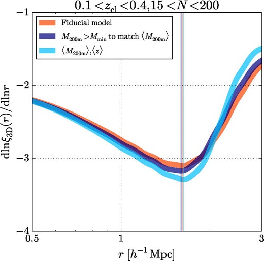
Comparison of model predictions for the logarithmic derivative of the three-dimensional cross-correlation function with the best-fitting mass–richness relation parameters for the clusters at 0.1 ≤ zcl ≤ 0.4 with 15 ≤ N ≤ 200 in Murata et al. (2019) from the fiducial analysis under the Planck cosmology. “Fiducial model” shows our fiducial model in equation (A1) that fully accounts for the scatter in the mass–richness relation, “M200m > Mmin to match 〈M200m〉” for the method in More et al. (2016), and “〈M200m〉, 〈z〉” for the method in Zürcher and More (2019) (see the text for more details). The vertical lines show the three-dimensional splashback radius location |$r_{\rm sp}^{\rm 3D}$| for each method. (Color online)
We note that Shin et al. (2019) checked the scatter effect by simulated halos with their selection accounting for scatters in their mass-observable relations and found results that are similar to our results shown in figure 12, albeit for more massive halos.
Appendix 3. Model parameter constraint contours
We show the model parameter constraint contours in figure 13 from the fiducial analysis with the full sample of 0.1 ≤ zcl ≤ 1.0 and 15 ≤ N ≤ 200 in table 1 to show the marginalized one-dimensional posterior distributions from each parameter and the |$68\%$| and |$95\%$| credible level contours for each two-parameter subspace from the MCMC chains.
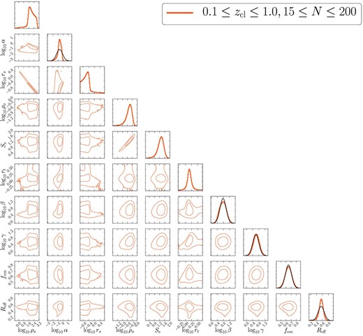
Model parameter constraints in the fiducial analysis for the full sample with 0.1 ≤ zcl ≤ 1.0 and 15 ≤ N ≤ 200 in table 3. Diagonal panels show the posterior distributions of the model parameters, and the other panels show the |$68\%$| and |$95\%$| credible level contours in each two-parameter subspace from the MCMC chains. Black lines show the Gaussian prior distributions in table 2. (Color online)
Footnotes
We use λ to denote richness for the redMaPPer-like cluster-finding algorithms.
We define the halo–matter cross-correlation function |$\xi _{\rm hm}^{\rm 3D}(r; M, z)$| as |$\rho (r; M, z)=\bar{\rho }_{\rm m0}[1+\xi _{\rm hm}^{\rm 3D}(r; M, z)]$|, where ρ(r; M, z) is the average matter density profile around halos with mass M at redshift z and |$\bar{\rho }_{\rm m0}$| is the present-day mean matter density. We note that we use the present-day mean matter density because we use the comoving coordinate for the radius and density in this paper.
References
