


Abstract
We investigated the properties of active galactic nucleus (AGN) environments, particularly environments where the association of a luminous galaxy (LG) is found within 4 Mpc from an AGN with redshift 0.8–1.1. For comparison, three additional AGN environments, (namely, AGNs of all types, type 1 AGNs with X-ray and/or radio detection, and type 2 AGNs) and an environment of blue M*, the characteristic luminosity of the Schechter function, galaxies were investigated. The cross-correlation function with the surrounding galaxies was measured and compared between the AGN and blue galaxy samples. We also compared the distributions of color, absolute magnitude, and stellar mass of the galaxies around such target objects. The properties of clusters detected using surrounding galaxies selected based on a photometric redshift were examined and compared for different samples. The target AGNs were drawn from the Million Quasars (MILLIQUAS) catalog, and the blue galaxies were drawn from six redshift survey catalogs (SDSS, WiggleZ, DEEP2, VVDS, VIPERS, and PRIMUS). The galaxies used as a measure of the environment around the targets were drawn from the S18a internal data released by the Hyper Suprime-Cam Subaru Strategic Program. We found that, among the five AGN and blue galaxy samples considered, the environment of AGN–LG pairs is the most enriched with luminous galaxies. We also found an enhancement in the number of mass-selected clusters in the AGN–LG pair sample against those in the other samples. The results obtained in this study indicate that existence of multiple clusters is the major driver in the association of AGNs and LGs, rather than a single large-mass dark matter halo hosting the AGN.
1 Introduction
The ubiquity of supermassive black holes (SMBHs) at the centers of galaxies has been recognized through the observation of nearby galaxies (Richstone et al. 1998; Kormendy & Ho 2013). Various processes are believed to be relevant to the feeding of SMBHs, including the following: secular evolution caused by gravitational instability inside a galaxy (Kormendy & Kennicutt 2004), a minor/major merger (Sanders et al. 1988; Di Matteo et al. 2005; Hopkins et al. 2008), quiescent accretion of hot halo gas (Kereš et al. 2009; Fanidakis et al. 2013), ram pressure (van den Bosch 2008), and tidal force feeding.
Low and intermediate luminosity AGNs are thought to be mostly caused by secular evolution, and the most luminous AGNs, i.e., quasi-stellar objects (QSOs), are triggered by major mergers (e.g., Treister et al. 2012; Menci et al. 2014). Several observations, however, have indicated that the major mergers are not a dominant mechanism for the triggering of a QSO (e.g., Villforth et al. 2017). The main driving mechanism of QSO activity remains open to debate.
One of the powerful ways to distinguish among the possible mechanisms is environmental analysis of the AGN (e.g., Coil et al. 2007, 2009; Hickox et al. 2009, 2011; Krumpe et al. 2012, 2018; Komiya et al. 2013; Ikeda et al. 2015; Shirasaki et al. 2018; He et al. 2018). Mergers are likely to occur in a high-density region except for a cluster core, where the relative velocity is too high to merge or interact with other galaxies and trigger gas accretion. The quiescent accretion of hot halo gas may be found in a cluster core, whereas ram pressure feeding occurs in the in-fall region of a cluster and between clusters that are in the process of merging. Thus, knowing the positional relationship between AGNs and high-density regions provides a hint to solving the present problem.
The Hyper Suprime-Cam Subaru Strategic Program (HSC-SSP) is a multi-band imaging survey conducted using the HSC (Miyazaki et al. 2012, 2018; Komiyama et al. 2018; Kawanomoto et al. 2018; Furusawa et al. 2018). The dataset of the wide layer covers 1400 deg2, and the limiting magnitude is as deep as r ∼ 26. Thus, it provides a powerful tool to investigate the environment of an AGN with unprecedented statistics.
Using the first-year dataset of HSC-SSP, Shirasaki et al. (2018) measured the clustering of galaxies around AGNs, and found that luminous galaxies are strongly clustered around them. Their results indicate that the cross-correlation length increases from 7 h−1 Mpc at approximately Mλ310 = −19 mag to >10 h−1 Mpc beyond Mλ310 = −20 mag, where Mλ310 represents the absolute magnitude measured at the rest frame wavelength of 310 nm. At approximately Mλ310 = −22 mag it reaches 30 h−1 Mpc, which is too large to be attributed solely to the mass of the host dark matter halo; the expected number density of dark matter haloes clustered at the same level of those luminous galaxies is too low to produce the observed number of luminous galaxies. Thus, the large clustering of luminous galaxies should be attributed in part, or mostly, to other properties related with their environment.
Shirasaki et al. (2018) also showed that the luminosity function measured around AGNs can be described using a smaller (brighter) characteristic luminosity parameter, M*, when fitted with the Schechter function (Schechter 1976). This indicates that the mass assembly of galaxies rapidly progress around some of the AGNs and, as a result, AGNs are more likely to be associated with luminous galaxies. As the strong cross-correlation between AGNs and luminous galaxies extends over the ∼10 Mpc scale, the mechanism should be related to the activity in a large-scale structure, such as a cluster–cluster interaction, enhanced galaxy merger, or gas inflow at a saddle point in the filament, among other possibilities. To understand what mechanism is relevant to the simultaneous occurrence of AGN activity and the evolution of galaxies around it, it is crucial to investigate the properties of the environment of the AGN, particularly an AGN with an association of luminous galaxies.
For this reason, we investigated the environmental properties around AGNs associated with luminous galaxies (LGs) within a distance of 4 Mpc (namely, AGNs paired with LGs, which are hereafter referred to as AGN–LG pairs) by comparing with the environment of four different target objects: blue galaxies, AGNs as a whole, type 1 AGNs through X-ray and/or radio detection (AGN type 1 XR), and type 2 AGNs. To determine the distance scale for selecting AGN–LG pairs we examined the clustering of galaxies around the pairs for three different scales, 2 Mpc, 4 Mpc, and 8 Mpc, and found that the significance of the excess of clustering against the whole AGN sample was the largest for the sample selected with the 4 Mpc scale. Thus, we decided to use 4 Mpc for selecting AGN–LG pairs for this study. The blue galaxies are used as a proxy for the environment of an ordinary galaxy.
Because different clustering properties have been reported for different types of AGNs by numerous authors (e.g., Hickox et al. 2009; Allevato et al. 2014; Mendez et al. 2016), we also carried out a comparison between different types of AGNs. In those studies, AGNs selected by X-ray and radio observations show larger clustering compared to the other types of AGNs. Thus, the AGN type 1 XR sample is used as representative of AGNs in higher overdensity environments. The clustering of LGs around AGNs increases at higher redshifts (Shirasaki et al. 2018), whereas the availability of galaxies measured for their redshift is limited to a redshift of ∼1.1 for the galaxy redshift catalogs used in this work: SDSS DR14 (Abolfathi et al. 2018), WiggleZ final (Drinkwater et al. 2018), DEEP2 DR4 (Newman et al. 2013), VVDS (Le Févre et al. 2013), VIPERS (Scodeggio et al. 2018), and PRIMUS (Coil et al. 2011; Cool et al. 2013). Thus, the target redshift was set to 0.8–1.1, where the sample size for AGN–LG pairs becomes maximal. From the results obtained through the comparisons, we aim to determine what type of mechanism has an effect on the AGN activity and the formation of LGs around the AGN.
Throughout this paper we assume a cosmology with Ωm = 0.3, Ωλ = 0.7, h = 0.7, and σ8 = 0.8. All magnitudes are given in the AB system. All distances are measured in comoving coordinates. The correlation length is presented in units of h−1 Mpc to facilitate a comparison with other measurements.
2 Datasets
2.1 Galaxies as a measure of the environment
As a measure of the environment of the AGNs and blue galaxies considered, we used photometric galaxies derived from the HSC-SSP survey. The internal release of the S18a wide layer dataset was used in this analysis. The observed locations and effective area of the S18a wide dataset are summarized in table 1. The typical depths of the observations are 26.6, 26.2, 26.2, 25.3, and 24.5 for the g, r, i, z, and y bands, respectively. The details of the survey itself are described in Aihara et al. (2017), and the content of the S18a dataset is provided in Aihara et al. (2019).
Summary of the survey area.
| Field name | Approx. center | S* |
|---|---|---|
| coordinates | (deg2) | |
| WIDE12H/GAMA15H | 13h10m, +00°00′ | 263.1 |
| VVDS | 23h20m, +02°00′ | 248.4 |
| GAMA09H | 09h35m, +02°00′ | 196.9 |
| XMM-LSS | 02h15m, −01°00′ | 132.5 |
| HECTOMAP | 15h00m, +43°30′ | 98.4 |
| WIDE01H | 01h15m, +01°00′ | 27.9 |
| AEGIS | 14h17m, +52°30′ | 2.1 |
| Total | 969.3 |
* Effective area of each survey field of S18a internal release.
The S18a dataset was analyzed through the HSC pipeline (version 6.5.1/6.5.3/6.6) developed by the HSC software team (Bosche et al. 2018) using software from the Large Synoptic Survey Telescope (LSST) pipeline (Ivezić et al. 2008; Axelrod et al. 2010; Jurić et al. 2015). Photometric and astrometric calibrations were conducted based on data obtained from the Panoramic Survey Telescope and Rapid Response System (Pan-STARRS) 1 imaging survey (Schlafly et al. 2012; Tonry et al. 2012; Magnier et al. 2013).
The photometric magnitude used in this work is a CModel magnitude. The galactic reddening was corrected according to the dust maps derived by Schlegel, Finkbeiner, and Davis (1998). There is a known issue regarding the CModel magnitude that, for some objects, the CModel magnitude has a significantly large deviation from other magnitude measurements, such as the magnitude in the aperture. We checked the effect of such errors on our analysis, and found that it is negligibly small.
The HSC sources satisfying the criteria summarized in table 2 were selected. The criteria were tested for all four griz bands. Because the observations in the y band are shallower than those in the other bands, detection in the y band was not required to avoid bias against redder galaxies. In addition to these selection criteria, other selections such as those based on the absolute magnitude space and photometric redshift (photo-z) were applied. These additional selections will be described in the analysis method and results section.
Summary of selection criteria of HSC sources.
| Column name* | Constraint | Explanation of the column |
|---|---|---|
| [girz]_pixelflags_edge | IS NOT TRUE | Source is outside usable exposure region |
| [griz]_pixelflags_saturatedcenter | IS NOT TRUE | Saturated pixel in the source center |
| [griz]_pixelflags_bad | IS NOT TRUE | Bad pixel in the source footprint |
| [griz]_cmodel_flag | IS NOT TRUE | CModel fit failed |
| [griz]_cmodel_mag | IS NOT NULL | CModel magnitude |
| [griz]_cmodel_mag | BETWEEN 1 AND 90 | |
| [griz]_cmodel_magsigma | IS NOT NULL | Uncertainty of CModel magnitude |
| [griz]_cmodel_magsigma | BETWEEN 0 AND 0.2 | |
| i_mask_s18a_bright_objectcenter | IS NOT TRUE | Source center is close to BRIGHT_OBJECT pixels |
| isprimary | IS TRUE | True if this is primary data for this object |
* [griz] in the column name means that any corresponding columns of four HSC bands (g, r, i, and z) were tested for the selection. All columns except for i_mask_s18a_bright_objectcenter are from the s18_wide.forced table. In addition, i_mask_s18a_bright_objectcenter is from the s18_wide.masks table.
The S18a dataset also provides photo-z and the stellar mass for most of the sources as an ancillary catalog (Tanaka et al. 2018). We utilized the photo-z and stellar masses calculated using the Direct Empirical Photometry code (DEmp; Hsieh & Yee 2014). The photo-z and stellar mass were computed from HSC photometry using the empirical fitting method independently.
In figure 1 we compare the photo-z (zphoto) and spectroscopic redshifts (spec-z, zspect) drawn from SDSS DR14 (Abolfathi et al. 2018), WiggleZ final (Drinkwater et al. 2018), DEEP2 DR4 (Newman et al. 2013), VVDS (Le Févre et al. 2013), VIPERS (Scodeggio et al. 2018), and PRIMUS (Coil et al. 2011; Cool et al. 2013). The matching of the objects was performed by searching nearest neighbors within 1″ of the HSC sources. The comparisons were made for HSC sources with i-band magnitudes between 22 and 24 mag, with an average magnitude of 22.6 mag. This magnitude range was chosen to match with a typical brightness range in this work. The standard deviation of the differences is 0.084 after 3 σ clipping for objects of zphoto = 0.8–1.1, and the fraction of outliers is 18% if it is defined as the fraction of |zspect − zphoto| > 0.1.
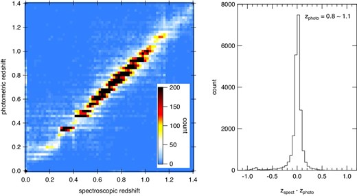
Comparison of photo-z derived from HSC photometric data and spec-z drawn from redshift catalogs of SDSS DR14, WiggleZ, DEEP2 DR4, VVDS, VIPERS, and PRIMUS. The left panel shows a density plot of photo-z vs. spec-z. The right panel shows a histogram of the difference between the two redshifts for objects at a photo-z of 0.8–1.1. (Color online)
The averages of the errors in the estimates of stellar mass are plotted in figure 2 for lower and upper bounds of 68% confidence interval. The error in the stellar mass is 0.1 dex at Ms = 109–1011 |$M_{\odot }$|, whereas the error in the lower bound rapidly increases above 1011.5 |$M_{\odot }$|.
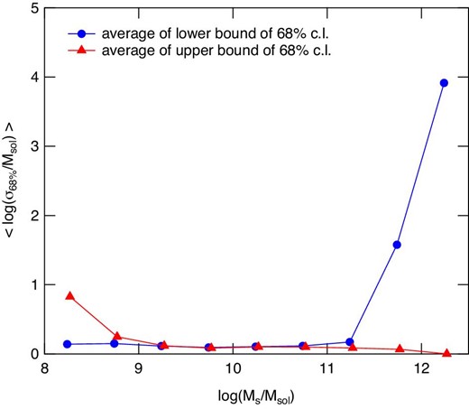
Averages of errors in the estimates of stellar mass for lower (solid circles connected with lines) and upper (solid triangles connected with lines) bounds of 68% C.L. interval in log Ms/|$M_{\odot }$|. (Color online)
2.2 AGN samples
The AGNs were drawn from the Million Quasars (MILLIQUAS) catalog v5.7 2019 update (Flesch 2015). MILLIQUAS is a compilation of identified AGNs/QSOs or candidates from various studies and QSO catalogs, which have reached 1983749 in number. We selected AGNs for which spec-z are within the range of 0.8–1.1 and that are well contained within the area of the S18a HSC-SSP wide dataset. The selected AGNs were further filtered according to the conditions of the HSC sources around them and their proximity, as described in subsection 2.4.
We extracted four AGN samples, namely, AGNs from all types (hereafter referred to as a whole AGN sample or simply an AGN sample), AGNs with an associated nearby (Mλ310 < −21) luminous galaxy (an AGN–LG pair sample or simply an AGN–LG sample), type 1 AGNs through X-ray or radio emissions (an AGN type 1 XR sample), and type 2 AGNs (an AGN type 2 sample). The absolute magnitude Mλ310 distributions for these AGN samples are shown in figure 3. The method for calculating the absolute magnitude is the same as that described in Shirasaki et al. (2018), and is detailed in the following section as well. For some of the AGNs, we were unable to measure Mλ310 owing to a saturation in the HSC photometry or other selection criteria preventing the source being analyzed. Such AGNs are counted in the brightest bin at Mλ310 = −28.0 to −27.8.
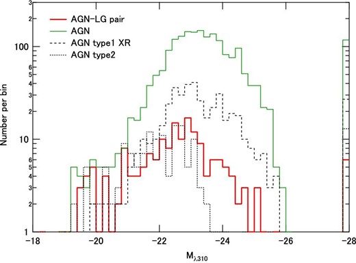
Distribution of absolute magnitude Mλ310 for each AGN sample. AGNs for which the absolute magnitude was not measured owing to saturation or other selection criteria are counted in the brightest bin. (Color online)
To see the difference in the distributions of the absolute magnitude between the AGN–LG sample and whole AGN sample, their number ratios are plotted in figure 4. The result shows that the AGNs in the AGN–LG sample are dominated by lower-luminosity AGNs as compared to those in the whole AGN sample.
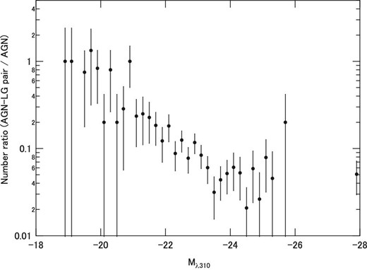
Ratio of the number of AGNs in the AGN–LG sample to their number in the whole AGN sample at each absolute magnitude Mλ310.
In constructing the sample of AGN–LG pairs, LGs were drawn from the following six redshift survey catalogs: SDSS DR14 (Abolfathi et al. 2018), WiggleZ final (Drinkwater et al. 2018), DEEP2 DR4 (Newman et al. 2013), VVDS (Le Févre et al. 2013), VIPERS (Scodeggio et al. 2018), and PRIMUS (Coil et al. 2011; Cool et al. 2013). These catalogs were also used for constructing the blue galaxy sample.
The absolute magnitude Mλ310 in these catalogs was measured for each galaxy, as described in the following section. The counterpart LGs were searched within 4 Mpc in projected distance from the AGN and 5 Mpc in the line-of-sight direction determined from the redshift measurement. The line-of-sight distance was set 1 Mpc larger to accommodate the redshift uncertainty. The typical redshift uncertainties 0.00006 (DEEP2), 0.0003 (SDSS, WiggleZ), 0.001 (VIPERS), 0.0014 (VVDS), and 0.01 (PRIMUS). Considering that 50% of the the AGN–LG pairs come from the DEEP2, SDSS, or WiggleZ catalogs, the margin of distance was chosen to be 1 Mpc, which corresponds to a redshift interval of 0.0004. The distribution of the separation distances to the brightest LGs is shown in figure 5.
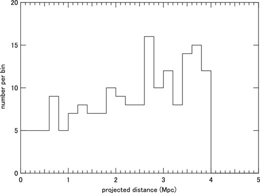
Distribution of projected separation distance between AGN and LG in the AGN–LG pair sample.
To reduce the effect of the redshift dependence of the clustering and other environmental properties in the comparison among the different samples, a redshift-match selection was carried out by selecting the same relative number of target objects at random for each redshift range of z = 0.8–0.9, 0.9–1.0, and 1.0–1.1. The relative numbers were determined from the numbers in the AGN–LG sample, which are 76, 54, and 50 for those redshift ranges, respectively. The details of the sample selections other than those described here are provided in subsection 2.4.
Summary of the numbers of each AGN type for four AGN samples.
| Type | Label* | |${{n}_{\textrm{AGN}}}^{\dagger }$| | |${n_{\textrm{AGN--LG}}}^{\ddagger }$| | |$n_{\textrm{Type1-XR}}$| § | |${n_{\textrm{Type2}}}^{\Vert }$| | ||
|---|---|---|---|---|---|---|---|
| AGN | type I | A | 21 | 11 | 0 | 0 | |
| X-ray | AX | 12 | 4 | 16 | 0 | ||
| type II | N | 11 | 10 | 0 | 17 | ||
| X-ray | NX | 27 | 12 | 0 | 36 | ||
| Radio | NR | 1 | 0 | 0 | 1 | ||
| X & Radio | NRX | 1 | 0 | 0 | 1 | ||
| QSO | type I | Q | 1420 | 37 | 0 | 0 | |
| X-ray | QX | 314 | 93 | 363 | 0 | ||
| Radio | QR,QR2 | 53 | 0 | 51 | 0 | ||
| X & Radio | Q2X,QRX,QR2X | 20 | 1 | 20 | 0 | ||
| type II | K | 59 | 7 | 0 | 70 | ||
| X-ray | KX | 16 | 4 | 0 | 23 | ||
| Radio | KR | 1 | 0 | 0 | 1 | ||
| X & Radio | KRX | 0 | 1 | 0 | 1 | ||
| Total | 1956 | 180 | 450 | 150 | |||
* Cassification of the object in the MILLIQUAS catalog: Q = QSO type I, A = AGN type I, K = narrow line QSO type II, N = narrow line AGN type II, R = radio association, X = X-ray association, 2 = double radio lobes.
† Number in the whole AGN sample.
‡ Number in the AGN–LG pair sample.
§ Number in the AGN type 1 XR (X-ray and/or radio detection) sample.
‖ Number in the AGN type 2 sample.
2.3 Blue M* galaxies
The blue M* galaxies were drawn from the following six redshift survey catalogs: SDSS DR14, WiggleZ final, DEEP2 DR4, VVDS, VIPERS, and PRIMUS. We selected galaxies located within the HSC-SSP wide area and within the redshift range of 0.8–1.1. This sample is used as representative of ordinary galaxies located in a relatively smaller density field than those of the AGNs and red galaxies.
We identified the HSC sources corresponding to those galaxies, and measured their color and absolute magnitude using the HSC photometric data. The measurement was made by fitting the galaxy spectral energy distribution (SED) templates to the observed SEDs using the EAZY software developed by Brammer, van Dokkum, and Coppi (2008). The absolute magnitude Mλ310 was measured at the rest frame wavelength of 310 nm, and the color was defined as D = Mλ270 − Mλ380, where Mλ270 and Mλ380 are the absolute magnitudes at 270 nm and 380 nm, respectively.
We then selected blue M* galaxies that satisfy the criteria Mλ310 ≥ −21 and D < 1.4. As shown in the later results section, the color distribution for galaxies is well represented with a linear combination of three Gaussian functions, which represent blue clouds, red sequences, and green valley galaxies. The criterion D < 1.4 separates most of the red galaxies from the sample.
In addition to the selections based on the properties of the target itself, the coverage and uniformity of the HSC sources around the targets were taken into account. As conducted for the AGN samples, a redshift-match selection was applied. Further details of the sample selection beyond those explained here will be described in subsection 2.4. In total, 2426 blue M* galaxies were used in this analysis. The number of galaxies from each survey is summarized in table 4.
Summary of the number of galaxies from each survey for the blue galaxy sample.
| SDSS | WiggleZ | DEEP2 | VVDS | VIPERS | PRIMUS | Total |
|---|---|---|---|---|---|---|
| 106 | 56 | 430 | 123 | 946 | 765 | 2426 |
| SDSS | WiggleZ | DEEP2 | VVDS | VIPERS | PRIMUS | Total |
|---|---|---|---|---|---|---|
| 106 | 56 | 430 | 123 | 946 | 765 | 2426 |
2.4 Dataset selection
In the analysis described here, we treated each target object (AGN or blue galaxy) and its surrounding HSC sources as a set. Hereafter, we refer to the unit of the dataset simply as a dataset. In this section we describe the criteria to include in the datasets for analysis.
To homogenize the environments of the target objects as much as possible and avoid edge effects at the survey boundary, we selected target objects that are well within the survey footprint. To do so, we measured the radial distribution of random sources from the positions of the target objects. The random source catalog is available for every data release. The random sources were generated with a density of 100 arcmin−2 inside the survey footprint, allowing us to estimate the fraction of unobserved or masked regions by counting the random sources.
We selected the random sources using the same criteria adopted for the real data if applicable. Their radial distribution was measured in annuli spaced by 0.2 Mpc out to 10 Mpc from the targets. We kept only those targets around which >60% of the area of all annuli at ≥2 Mpc and >80% of the area at <2 Mpc were included in the survey footprint and not masked for bright sources. The procedure to build and validate the bright-star masks for the HSC-SSP survey is described in Coupon et al. (2018). The datasets that passed this selection numbered 2740 for the AGNs and 5222 for the blue galaxies.
The spatial uniformity of the HSC sources around the targets was also examined to identify datasets significantly affected by a high-density foreground region, spurious sources around bright stars, and so on. For this purpose, we calculated two parameters for the radial number density distribution of the galaxies, χ2 and σmax, where χ2 is the square sum of the deviation from the number density distribution fitted to the observed data using equation (5), which is derived in subsection 3.1, and σmax is the maximum deviation from the density distribution. The criteria adopted for these parameters were as follows: χ2/n ≤ 4 and σmax ≤ 6. These criteria were chosen to remove the few percent of the datasets that deviate the most from a uniform distribution. We checked the effect of these criteria on the estimate of cross-correlation length and confirmed that the difference between the cross-correlation lengths calculated for the datasets for which these selections were adopted or not is within the statistical error. The datasets that passed all selections described above totaled 2720 for the AGNs and 5126 for the blue galaxies.
In the analysis used for this study, it is crucial to construct the datasets such that the contributions from the foreground and background galaxies are smeared out by stacking the radial number distributions of the galaxies. To avoid stacking numerous identical fields, we selected the target objects so that they had no more than one other target object within 4 Mpc. This selection was used for each redshift bin, which was divided into z = 0.8–0.9, 0.9–1.0, and 1.0–1.1. The datasets that passed all selections described above numbered 2622 for the AGNs and 4262 for the blue galaxies.
To reduce the effect of the redshift dependence in the comparison of the environmental properties, we selected the datasets such that the relative number of datasets for three redshift bins was the same among the five target groups. The final numbers of datasets that passed all selections are summarized in table 5, along with the median redshifts and absolute magnitudes of the datasets. The numbers of datasets broken down by HSC survey fields are also summarized in table 6.
Summary of the number, median redshift, and median absolute magnitude in the sample for each target type and each redshift group.
| z* | Sample type | n † | |$\tilde{z}^{\ddagger }$| | |$\tilde{M}_{\lambda 310}$| § |
|---|---|---|---|---|
| 0.8–0.9 | AGN | 826 | 0.85 | −23.0 |
| Blue galaxy | 1024 | 0.85 | −20.6 | |
| AGN–LG pair | 76 | 0.85 | −22.3 | |
| AGN type 1 XR | 190 | 0.84 | −22.8 | |
| AGN type 2 | 63 | 0.85 | −21.7 | |
| 0.9–1.0 | AGN | 587 | 0.95 | −23.4 |
| Blue galaxy | 728 | 0.93 | −20.7 | |
| AGN–LG pair | 54 | 0.96 | −22.9 | |
| AGN type 1 XR | 135 | 0.96 | −23.2 | |
| AGN type 2 | 45 | 0.96 | −22.4 | |
| 1.0–1.1 | AGN | 543 | 1.05 | −23.8 |
| Blue galaxy | 674 | 1.04 | −20.7 | |
| AGN–LG pair | 50 | 1.03 | −22.9 | |
| AGN type 1 XR | 125 | 1.05 | −23.8 | |
| AGN type 2 | 42 | 1.04 | −22.6 | |
| 0.8–1.1 | AGN | 1956 | 0.92 | −23.3 |
| Blue galaxy | 2426 | 0.92 | −20.7 | |
| AGN–LG pair | 180 | 0.91 | −22.6 | |
| AGN type 1 XR | 450 | 0.93 | −23.2 | |
| AGN type 2 | 150 | 0.94 | −22.1 |
* Redshift range.
† Number of datasets.
‡ Median redshift.
§ Median absolute magnitude Mλ310. The median redshift and absolute magnitude for AGN–LG pairs are calculated for the AGN.
Summary of the number of datasets for each target type and HSC survey field.
| Field name | |${n_{\rm AGN}}^{*}$| | |${n_{\rm G}}^{\dagger }$| | |${n_{\rm AGN\!-\!LG}}^{\ddagger }$| | |$n_{\rm Type1\mbox{-}XR}$| § | |${n_{\rm Type2}}^{\Vert }$| |
|---|---|---|---|---|---|
| WIDE12H/GAMA15H | 583 | 36 | 3 | 70 | 31 |
| VVDS | 490 | 626 | 38 | 58 | 13 |
| GAMA09H | 259 | 252 | 18 | 42 | 61 |
| XMM-LSS | 376 | 1358 | 102 | 211 | 44 |
| HECTOMAP | 166 | 0 | 3 | 26 | 0 |
| WIDE01H | 67 | 1 | 2 | 28 | 0 |
| AEGIS | 15 | 153 | 14 | 15 | 1 |
* Number in the whole AGN (for all types) sample.
† Number in the blue galaxy sample.
‡ Number in the AGN–LG pair sample.
§ Number in the AGN type 1 XR (X-ray and/or radio detection) sample.
‖ Number in the AGN type 2 sample.
3 Analysis method
3.1 Cross-correlation between targets and HSC sources
The cross-correlation functions between the target objects and HSC sources were calculated using the method described in our previous papers (Shirasaki et al. 2011, 2016, 2018; Komiya et al. 2013), which is briefly described here.
When the redshifts of the target objects are known, we can calculate the number densities of the HSC sources as a function of the projected distance from the target in its redshift plane. Thanks to the clustering properties of galaxies, the galaxies located at the target’s redshift emerge as an excess over the flat distribution of the foreground/background galaxies after stacking the radial number densities for many of the targets.
ρ0 for each dataset is calculated from the luminosity function, which was derived by parameterizing the luminosity functions in the literature, and the completeness function C(m). The detail of the parametrization of the luminosity function and the completeness function is described in Shirasaki et al. (2018); the completeness function is referred to as the detection efficiency DE(m) in the reference. The average for all the datasets in the sample provides ρ0 in equation (5).
The completeness as a function of magnitude, C(m), is required to correct for the completeness by multiplying the luminosity function model in deriving ρ0. It was calculated as the ratio of the observed magnitude distribution Nobs(m) to the model function Norg(m), which is the magnitude distribution expected for an ideal observation of 100% completeness at any magnitude. For Norg(m), we assumed a broken power-law form, and the power-law index was determined using data from the HSC-SSP S18a deep survey dataset of the COSMOS field. Next, C(m) was determined for each dataset by fitting C(m)Norg(m) to Nobs(m). For the model of C(m), the same functional form as defined in equation (14) of Shirasaki et al. (2018) was used.
The accuracy of the model function is demonstrated in figure 6 for the magnitude distribution derived from a deep dataset of the COSMOS field. The observed magnitude distribution is well fitted with the broken power-law model at magnitudes mλ310 < 26.8 mag. Since this work is performed at magnitudes mλ310 < 26 mag for the wide dataset, it is reasonable to assume a broken power-law form for Norg(m).
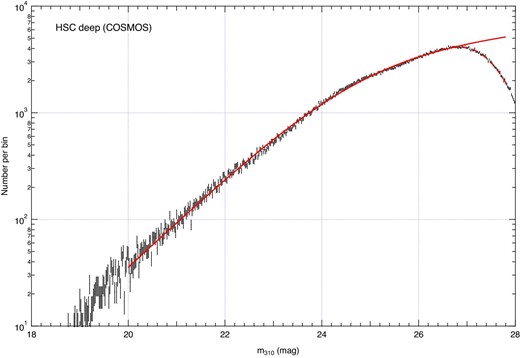
Distribution of apparent magnitude mλ310 derived from a deep dataset of the COSMOS field, where mλ310 is the apparent magnitude measured at a wavelength of 310(1 + 0.9) nm in the observer frame, that is, 310 nm in the rest frame at redshift 0.9. The solid and dashed lines represent the fitted function expressed in a broken power-law function and that multiplied by the completeness C(m), respectively. (Color online)
The radial distributions n(rp) of the HSC sources were derived by stacking the distributions for all the datasets in the sample, where HSC sources with absolute magnitudes of Mλ310 < −19 mag were used. This threshold magnitude corresponds to an approximately 90% detection (completeness) limit. We applied this analysis for the photo-z selected galaxies, which were constructed by selecting the HSC source whose photo-z was within ±0.1 of the redshifts of the target object. Although the completeness is reduced by this photo-z selection, background/foreground galaxies are also reduced more efficiently, which results in an increase in the signal-to-noise ratio of the clustering.
The reduction in the completeness by the photo-z selection was estimated by comparing the projected cross-correlation functions calculated for galaxies with and without photo-z selection. The two projected cross-correlation functions were calculated for the same ρ0 parameter, which was an estimate for the galaxies without a photo-z selection, and the average ratio between them was then taken to be the reduction rate due to the photo-z selection. The reduction rate was estimated to be 0.61 for the whole AGN sample, which has a large statistical sample size and provides the best signal-to-noise ratio for the clustering, and was also used for the other samples. In figure 7, the two projected cross-correlation functions used to derive the reduction rate are shown.
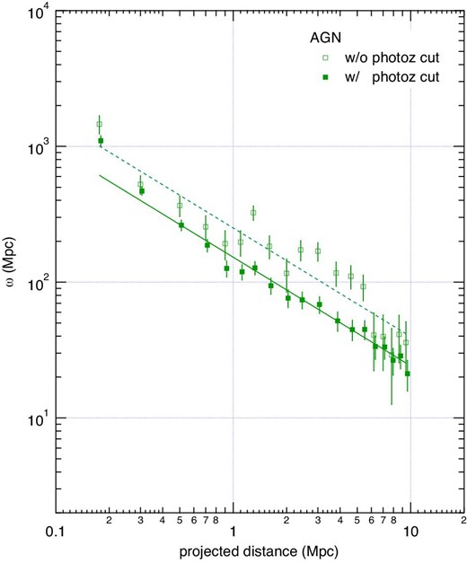
Projected cross-correlation functions for the whole AGN sample. The open squares indicate the correlation function obtained using all of the galaxies, whereas the solid squares represent that obtained using the photo-z selected galaxies. The same ρ0 parameter, which was estimated without correcting the reduction through a photo-z selection, is used for both. We use the ratio between them as the correction factor for the photo-z selection. (Color online)
The effective observational area, which is used for the calculation of n(rp) and is the area corrected for dead regions affected by a bright source, the survey boundary, gaps between observations, or other factors, was estimated using a random catalog. The random catalog, which was created at random positions avoiding the dead region with number density 100 arcmin−1, was extracted from the S18a database.
We fixed γ at 1.8, and the model function given by equation (5) was fitted to the observed radial surface densities n(rp) with two free parameters, r0 and nbg. The fitting was performed by the least squares method by weighting each data point with the inverse square of the error determined by Poisson statistics. Since the target objects were selected so as to avoid overlap of the environment regions between them as much as possible, the bins of n(rp) are almost independent of each other and the covariance between them is negligible. Thus, we ignored the covariance in the fitting. The cross-correlation length was estimated as the optimal solution for the free parameter r0. The quoted error is a 1 σ confidence interval unless otherwise stated.
We also cross-correlated the target objects to the cluster of HSC sources. Because no reliable model is available for the cluster mass function, we simply derived the radial number density of the clusters.
3.2 Color, absolute magnitude, and stellar mass distributions around the targets
Although we do not have spec-z for individual HSC sources, we can statistically estimate the distribution of a property X of the HSC sources located at a distance within a few Mpc of the target object. Thanks to the clustering feature of galaxies, their number density increases as we get closer to the target objects. Thus, subtracting the distribution of property X measured in a lower-density region from that measured in a higher-density region, we can estimate the net distribution of property X for HSC sources associated with the target objects.
Property X can be anything that is measurable for the HSC sources. In this analysis, we investigate the distribution of color, absolute magnitude, and stellar mass of the HSC sources. The color is calculated as the difference between magnitudes at the rest frame wavelengths of 270 and 380 nm, and the absolute magnitude is measured at 310 nm in the rest frame of the target object. As previously described in subsection 2.3, the EAZY software (Brammer et al. 2008) was used to interpolate the SED derived from the HSC photometric data. The stellar mass was obtained from the ancillary catalog available along with the photo-z. We used those calculated using DEmp (Hsieh & Yee 2014). Photo-z was used to select HSC sources associated with the target objects.
Although the photo-z selection is useful for increasing the signal-to-noise ratio of the derived distribution, it distorts the intrinsic distribution because of the dependence of the completeness on the examined property. Thus, the completeness should be corrected taking into account its dependence on the property, when the distribution needs to be compared in an absolute manner, e.g., in a case where it is compared with the luminosity functions derived in the literature. The reduction rate by photo-z selection as a function of the absolute magnitude is estimated by comparing the magnitude distribution obtained for all galaxies (without photo-z selection) with that for the photo-z selected galaxies of the whole AGN sample.
In addition, we also investigated the peak density distribution of the clusters detected as stellar mass density peaks (mass peak clusters) and clusters detected as number density peaks (number peak clusters), which were found using a procedure for detecting peaks in the two-dimensional (2D) distribution of the HSC sources.
3.3 Identification of peak locations of galaxy number density and stellar mass density around the targets
As described in section 1, the strong cross-correlation between AGNs and LGs found by Shirasaki et al. (2018) extends over a ∼10 Mpc scale, which indicates that the mechanism is related to the activity in the large-scale structure. A cluster–cluster interaction is one candidate to produce strong cross-correlation at such a large scale. Thus, we examined the environment of AGN–LG pairs based on the statistics related to the clusters around them.
The peak locations of the number density and stellar mass density of the HSC sources were detected to select galaxy cluster candidates by searching for local maxima in a blurred density map. The blurred density map was constructed by blurring the positional distribution of the photo-z selected HSC sources using a 2D Gaussian with σ = 1 Mpc. The stellar mass density map was created by weighting each HSC source with its stellar mass, whereas the number density map was created with an equal weight. The stellar mass was limited to 10|$^{12}\, M_{\odot }$| to avoid dominance from a single large stellar mass object with a large uncertainty, as shown in figure 2, and thus a stellar mass exceeding 10|$^{12}\, M_{\odot }$| was set to 10|$^{12}\, M_{\odot }$|. We checked that lowering the threshold to |$10^{11.5}\, M_{\odot }$| does not affect the result and conclusion. Local sub-peaks found within a 1 Mpc projected distance from the local maximum were removed from the sample.
4 Results
4.1 Cross-correlation between target objects and HSC sources
The cross-correlations between the target objects and the HSC sources were examined for five target types: whole AGN (of all types), blue galaxy, AGN–LG pair, AGN type 1 XR (with detection with X-ray and/or radio signals), and AGN type 2.
The results of the fitting and the fixed parameters are summarized in table 7. The cross-correlation functions obtained using the fitting parameters are shown in the left panel of figure 8 for the cases of the whole AGN, blue galaxy, and AGN–LG samples, and in the right panel for the cases of AGN type 1 XR and AGN type 2 samples. The cross-correlation lengths obtained for the five samples are compared in figure 9. The cross-correlation lengths obtained for the whole AGN, AGN type1 XR, and AGN–LG samples are significantly larger than those for the blue galaxy and AGN type 2 samples.
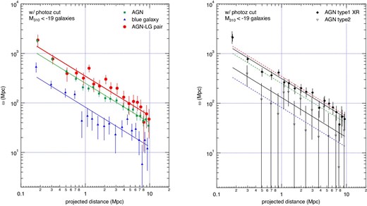
Left: Projected cross-correlation functions derived for the whole AGN, blue galaxy, and AGN–LG pair samples. The solid lines indicate the power-law functions fitted to the data points. The photo-z selected galaxies were used and the data were corrected for a reduction in the factor of 0.61. Right: The same plots as the left panel for the AGN type 1 XR (X-ray and/or radio detection) and AGN type 2 samples. The solid lines are the functions fitted to the data of these two samples, and the dashed lines are the functions fitted to the whole AGN, AGN–LG, and blue galaxies, as shown in the left panel with the solid lines. (Color online)
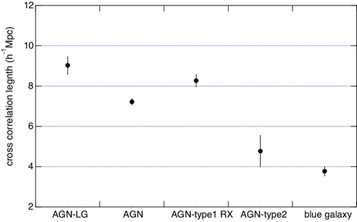
Cross-correlation lengths measured for the five targets.
Fitting parameters of cross-correlation functions between five types of target and HSC sources.
| Target type | n* | 〈z〉† | |${r_0}^{\ddagger }$| | |$n_{\mathrm{bg}}$| § | |${\rho _{0}}^{\Vert }$| | γ♯ |
|---|---|---|---|---|---|---|
| (h−1 Mpc) | (Mpc−2) | (10−3 Mpc−3) | ||||
| AGN–LG pair | 180 | 0.93 | 9.03 ± 0.44 | 4.807 ± 0.019 | 3.01 | 1.8 |
| AGN | 1956 | 0.93 | 7.22 ± 0.16 | 4.695 ± 0.006 | 2.92 | 1.8 |
| Blue galaxy | 2426 | 0.93 | 3.77 ± 0.27 | 4.747 ± 0.005 | 3.02 | 1.8 |
| AGN type-1 RX | 450 | 0.93 | 8.27 ± 0.31 | 4.718 ± 0.012 | 2.90 | 1.8 |
| AGN type-2 | 150 | 0.94 | 4.77 ± 0.78 | 4.890 ± 0.020 | 3.04 | 1.8 |
* Number of target objects.
† Average redshift.
‡ Cross-correlation length and its 1 σ error.
§ Average surface number density.
‖ Average space number density of galaxies at the redshift of the targets.
♯ Power index fixed to 1.8.
The cross-correlation length for the AGN–LG sample is larger than that for the whole AGN sample by 4 σ, and is identical to that for the AGN type 1 XR sample within the margin of error. The environment of AGN type 2 is similar to that of the blue galaxies, which indicates that the AGNs of this sample are mostly caused by an internal secular mechanism rather than an interaction with the external environment.
4.2 Color distributions
To investigate the difference in the composition of the galaxy types clustered around the three target types, namely, the whole AGN, blue galaxy, and AGN–LG pairs, we derived the distribution of galaxy color within the region 0.2–2.0 Mpc from the targets. For simplicity, in the subsequent analysis, excluding the average number of clusters around the targets, the comparisons are made only for the three samples.
The color distribution was obtained by subtracting the color distribution in a lower-density region (7–9.8 Mpc) from that in a higher-density region (0.2–2.0 Mpc). The color of each HSC source was calculated according to the method described in subsection 3.2. The distributions were derived from the HSC sources with magnitude brighter than Mλ320 = −19 mag and selected based on their photo-z. The results are shown in figure 10.
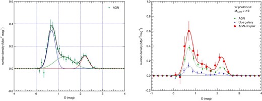
Left: Color distributions of photo-z selected galaxies around the AGNs of the whole AGN sample. The distributions were fitted using a linear combination of three Gaussian functions, each of which corresponds to blue-, green-, and red-type galaxies. Right: Color distributions of photo-z selected galaxies around AGNs or blue galaxies for the samples of whole AGN, blue galaxy, and AGN–LG pairs. The distributions are fitted using three Gaussian functions.
Each color distribution was fitted with a linear combination of three Gaussian distributions, each of which represents the distribution for red sequence galaxies, blue cloud galaxies, and green valley galaxies. The fitting was first applied to the distributions for the whole AGN sample (left panel of figure 10) by making all nine parameters free. The fitting was then conducted by fixing the mean and standard deviation parameters of the three Gaussians to those determined with the fitting to the whole AGN sample (right panel of figure 10). The fitted function is shown in the figure and the values of the fitting parameters are summarized in table 8.
Fitting results for the color distributions.
| Target type | c* | |${\mu _{\mathrm{B}}}^{\dagger }$| | |${\sigma _{\mathrm{B}}}^{\ddagger }$| | |$f_{\mathrm{G}}$| § | |${\mu _{\mathrm{G}}}^{\dagger }$| | |${\sigma _{\mathrm{G}}}^{\ddagger }$| | |$f_{\mathrm{R}}$| § | |${\mu _{\mathrm{R}}}^{\dagger }$| | |${\sigma _{\mathrm{R}}}^{\ddagger }$| |
|---|---|---|---|---|---|---|---|---|---|
| AGN‖ | 0.304 ± 0.016 | 0.70 ± 0.02 | 0.17 ± 0.03 | 0.36 ± 0.13 | 1.25 ± 0.16 | 0.41 ± 0.13 | 0.16 ± 0.03 | 2.21 ± 0.03 | 0.17 ± 0.02 |
| AGN♯ | 0.304 ± 0.014 | 0.70 | 0.17 | 0.36 ± 0.03 | 1.25 | 0.41 | 0.16 ± 0.01 | 2.21 | 0.17 |
| AGN–LG pair♯ | 0.506 ± 0.049 | 0.70 | 0.17 | 0.33 ± 0.06 | 1.25 | 0.41 | 0.21 ± 0.03 | 2.21 | 0.17 |
| blue galaxy♯ | 0.093 ± 0.013 | 0.70 | 0.17 | 0.29 ± 0.08 | 1.25 | 0.41 | 0.17 ± 0.04 | 2.21 | 0.17 |
* Scaling factor of the Gaussian distribution for each galaxy component.
† Mean of the D distribution for each component.
‡ Standard deviation of the D distribution for each component.
§ Fraction of green or red galaxy component.
‖ Fitting was applied by making all nine parameters free.
♯ Fitting was applied by fixing the mean and standard deviation parameters to the values obtained for the nine-parameter fitting to the data of the whole AGN sample.
The number fractions of the green- and red-type galaxies to the total number of galaxies for the three samples are plotted in figure 11. There is no significant difference between them.
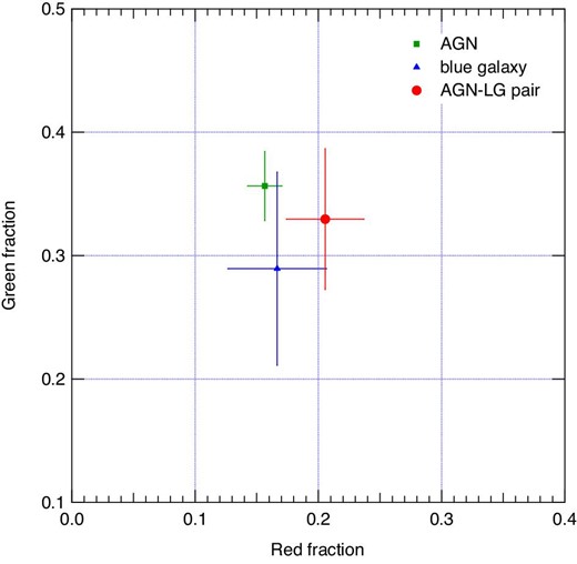
Fractions of red and green galaxies obtained for the three samples. (Color online)
4.3 Absolute magnitude distribution
To investigate the difference in the luminosity function of the galaxies clustered around the three target types, we derived the absolute magnitude distributions within the region 0.2–2.0 Mpc from the targets, as applied for the color in the previous section. They were derived separately for two galaxy types, namely, the blue and red galaxy types. The blue types were selected by their color D < 1.4, and the red types were selected using D ≥ 1.4. Because the color distribution of a green-type galaxy overlaps significantly with those of the red- and blue-type galaxies, we simply divided the data into two galaxy types. The absolute magnitude of each HSC source was calculated according to the method described in subsection 3.2.
The absolute magnitude distributions derived were corrected for completeness, including the reduction from the photo-z selection. To estimate the reduction rate by the photo-z selection as a function of the absolute magnitude, we compared the magnitude distribution obtained for all galaxies (without photo-z selection) with that for the photo-z selected galaxies of the whole AGN sample. The results are shown in figure 12. The top panel of the figure shows the comparison between the two galaxy samples, and the bottom panel shows the ratio of the photo-z selected galaxies to all galaxies.

Top: Absolute magnitude distributions of galaxies around AGNs for the whole AGN sample. The blue and red markers are distributions for the blue and red galaxies, respectively. The distributions shown with solid markers are derived from all galaxies, and those shown with open markers are from the photo-z selected galaxies. Bottom: Ratios for the number of photo-z selected galaxies against all galaxies. (Color online)
We assumed that the reduction rate for the red galaxy type is constant for the entire magnitude range. The measured ratios are consistent with this assumption and the average ratio obtained was 0.665. In the case of the blue galaxy type, the rate of reduction decreases on the fainter side, as shown in the bottom panel of figure 12, and thus we interpolated the ratios using an analytic function, such that it increases to the average ratio given for the red galaxy type. The interpolation is shown as a solid blue line in the same panel.
Using the reduction rate obtained in this way, we corrected the magnitude of the distributions derived from the photo-z selected galaxies for the three target types. The results are shown in figure 13. The plots are only shown in the magnitude range where the completeness exceeds 50%.
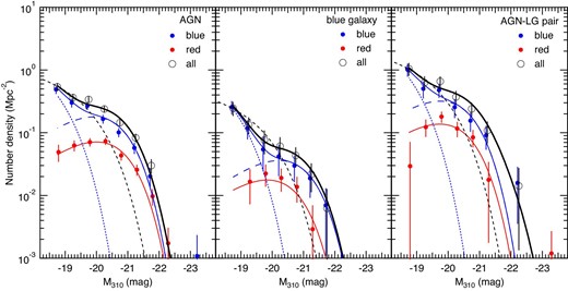
Absolute magnitude distributions of photo-z selected galaxies around target objects for three samples. The blue (red) closed circles indicate distributions for blue (red) galaxies, and the open circles are for all galaxies. The solid lines represent fitted functions expressed by a Schechter function (for red galaxies) or a combination of two Schechter functions (for blue galaxies). The thick lines represent the sum of the functions for blue and red galaxies. The dashed lines represent a model function derived from the luminosity functions described in the literature for z = 0.95, which are normalized to the data at Mλ310 = −18.75. The dotted and long-dashed lines represent fitted functions corresponding to the primary and secondary components of blue galaxies, respectively. (Color online)
The magnitude distributions are fitted with a single Schechter function (Schechter 1976) for the red galaxy type, whereas those for the blue galaxy type are fitted with a combination of two Schechter functions with different parameters. In fitting to the distributions for the red galaxy, we fixed the α parameter of the Schechter function to α = 0, which is the average obtained for the three targets by making the α parameter free. This is to compare M* among the three samples by fixing the α parameter to the same value. The fitting parameters are summarized in table 9.
Fitting result for absolute magnitude distribution of red galaxies.
| Target type | |${\phi _{\mathrm{R}}}^{*}$| | |${\alpha _{\mathrm{R}}}^{\dagger }$| | |${M_{*,\mathrm{R}}}^{\ddagger }$| | χ2§ | n ‖ |
|---|---|---|---|---|---|
| AGN | 0.026 ± 0.003 | 0.0 | −20.0 ± 0.07 | 3.59 | 7 |
| Blue galaxy | 0.007 ± 0.003 | 0.0 | −19.9 ± 0.27 | 5.54 | 7 |
| AGN–LG pair | 0.062 ± 0.013 | 0.0 | −19.7 ± 0.15 | 5.53 | 7 |
* Number density at Mλ310 = −18.
† α parameter of the Schechter function. This was fixed at 0.0.
‡ M * parameter of the Schechter function.
§ Normalized residual sum of squares.
‖ Number of data points.
Looking at the plot for the blue galaxy sample (middle panel of figure 13), the magnitude distribution for the blue galaxy type flattens at approximately Mλ310 ∼ −20 and steepens again at approximately Mλ310 ∼ −21. To reproduce this feature we assumed two components, one of which is characterized using the Schechter function with a larger (fainter) characteristic magnitude M* and slope parameter α = −1.2, and the other is characterized with a smaller (brighter) M* and flat slope parameter α = 0, which is the parameter used for the red galaxy type. In the cases of the whole AGN and AGN–LG samples, the secondary component with the brighter M* parameter dominates over the primary component at magnitudes Mλ310 < −19. Because of that, the parameter M* for the primary component was not well constrained, and thus the M* parameter was fixed to the value obtained for the blue galaxy sample.
In order to test the preference for adding the secondary component, we also fitted the absolute magnitude distribution with a single component model and calculated the Akaike information criterion (AIC) (Akaike 1974) and Bayesian information criterion (BIC) (Schwarz 1978) for both the single- and two-component models. The AIC and BIC are information criteria to evaluate the goodness of the statistical model from both the goodness of the fit and complexity of the model, and have been widely applied to astrophysics problems (e.g., Takeuchi 2000; Liddle 2007; Shirasaki et al. 2008).
Fitting result for absolute magnitude distribution of blue galaxies.
| Target type | |${\phi _{\mathrm{B1}}}^{\dagger }$| | |${\alpha _{\mathrm{B1}}}^{\ddagger }$| | |$M_{*,\mathrm{B1}}$| § | |${\phi _{\mathrm{B2}}}^{\dagger }$| | |${\alpha _{\mathrm{B2}}}^{\ddagger }$| | |$M_{*,\mathrm{B2}}$| § | χ2‖ | n ♯ | k** | AIC†† | BIC‡‡ |
|---|---|---|---|---|---|---|---|---|---|---|---|
| AGN | 0.96 ± 0.17 | −1.2 | −18.3 | 0.070 ± 0.012 | 0.0 | −19.90 ± 0.09 | 6.50 | 7 | 3 | 5.5 | 5.3 |
| 0.50 ± 0.05 | −1.2 | −20.6 ± 0.12 | — | — | — | 3.24 | 7 | 2 | −1.4 | −1.5 | |
| Blue galaxy | 0.56 ± 0.29 | −1.2 | −18.3 ± 0.56 | 0.011 ± 0.008 | 0.0 | −20.2 ± 0.35 | 0.05 | 7 | 4 | −26.6 | −26.8 |
| 0.19 ± 0.05 | −1.2 | −20.4 ± 0.31 | — | — | — | 6.23 | 7 | 2 | 3.2 | 3.1 | |
| AGN–LG pair | 1.84 ± 0.58 | −1.2 | −18.3 | 0.142 ± 0.054 | 0.0 | −19.7 ± 0.20 | 2.13 | 7 | 3 | −2.3 | −2.5 |
| 1.02 ± 0.18 | −1.2 | −20.3 ± 0.23 | — | — | — | 3.28 | 7 | 2 | −1.3 | −1.4 |
† Number density at Mλ310 = −18 for the primary (B1) and secondary (B2) components.
‡ α parameter of the Schechter function for the primary (B1) and secondary (B2) components; fixed to −1.2 and 0.0, respectively.
§ M * parameter of the Schechter function for the primary (B1) and secondary (B2) components. M*, B1 for the AGN and AGN–LG pairs are fixed to −18.3, which is the value obtained for blue galaxies.
‖ Normalized residual sum of squares.
♯ Number of data points.
** Number of free parameters.
†† Akaike information criterion.
‡‡ Bayesian information criterion.
According to the χ2 values, both models are acceptable at the 90% confidence level for all the samples. If we compare the AIC and BIC values between the two models for each sample, the two-component model is preferable for the blue galaxy and AGN–LG samples, and the one-component model is preferable for the whole AGN sample. This result supports introducing the second component to the model as a plausible scenario, especially for the blue galaxy sample. If this is the case, it is natural to expect that two components exist ubiquitously and there is a difference in the mixing ratio depending on the environment. The small difference in the AIC and BIC values for the AGN and AGN–LG samples compared to the blue galaxy sample can be considered as a result of the dominance of the secondary component, which is inferred from the two-component fit, in the examined magnitude range. In such a case AIC/BIC will preferentially select the single-component model.
The M* parameters obtained for the red-type galaxy and the secondary component of the blue-type galaxy are shown in figure 14. As indicated in the figure, there are no significant differences in the M* parameters among the three samples or between the blue and red types. Thus, the differences in the magnitude distribution among the three samples are the fraction of the secondary component in the blue galaxy type and the normalization factor of the luminosity function for each component.
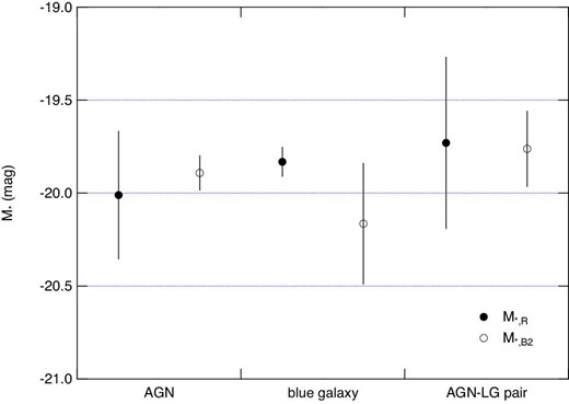
M * parameters obtained for the secondary component of blue galaxies (M*, B2) and for red galaxies (M*, R).
4.4 Stellar mass distribution
Stellar mass distributions around the target objects for three samples were derived using the photo-z selected HSC sources with absolute magnitude of Mλ310 < −19. Figure 15 shows a comparison between them. The top panel shows the number densities at distances of 0.2–2.0 Mpc from the target objects, which were obtained by subtracting the density distribution at 7–9.8 Mpc from that at 0.2–2.0 Mpc. The bottom panel shows the ratios to the number densities obtained for the whole AGN sample.
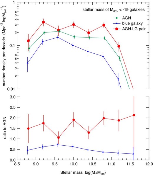
Top: Stellar mass distribution of galaxies around target objects of three samples. Bottom: Ratios of the densities to those measured for the whole AGN sample. (Color online)
It can clearly be seen that HSC sources around the targets in the whole AGN and AGN–LG samples have a higher relative density than those in the blue galaxy sample at stellar masses of |$M_{*} \ge 10^{10}\, M_{\odot }$|. The ratios for the blue galaxy sample show a decreasing trend above 10|$^{9.6}\, M_{\odot }$|. There is no significant difference in the ratios for the AGN–LG sample.
4.5 Positional distribution of clusters
In previous sections we compared the properties of the environment for three samples based on the properties of individual HSC sources, i.e., galaxies. In this and the following sections we investigate the properties of their environment, focusing on the clusters of the HSC sources.
The method used to find clusters is described in subsection 3.3. In creating the stellar mass or number density map, we used photo-z selected HSC sources with a magnitude of Mλ310 < −19 mag. We selected clusters based on two density maps: one is a map of the stellar mass density and the other is a map of the source number density.
Figure 16 shows the radial number density distributions of clusters found in the stellar mass density map (mass peak clusters, left-hand panel) and clusters found in the number density map (number peak clusters, right-hand panel). The threshold for the counting cluster was set to peak densities of |$10^{10.8}\, M_{\odot }\:$|Mpc−2 and 101.6 Mpc−2, respectively. These numbers correspond to the detection threshold for clusters by this method, as shown in figure 18 of the next section. The average cluster density at a projected distance of 4–7 Mpc are subtracted from the density distribution. In each panel, the distributions for the three samples are compared. The uncertainties of the number density are derived based on Poisson statistics and the error bars denote 1 σ uncertainty.
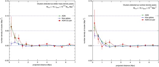
Left: Radial distributions of clusters detected as stellar mass density peaks for three samples. Offset (background) densities measured at 4–7 Mpc were subtracted. Right: As the left panel but for clusters detected as number density peaks.
The distributions of the mass peak clusters show an excess over the average at <1.2 Mpc, and the excess density increases toward the target objects for the cases of the whole AGN and AGN–LG samples. The significance of the excess is 7.1 and 2.9 σ for the whole AGN and AGN–LG samples, respectively. The excess is smaller and less significant (2.8 σ) for the blue galaxy sample.
The distributions of the number peak clusters show a significant excess at <1.2 Mpc distance for all three samples. The significance of the excess is 6.8, 2.6, and 7.3 σ for the whole AGN, AGN–LG, and blue galaxy samples, respectively. The number density distributions are almost identical among the three samples. The average number of clusters that have a peak number density of >101.6 Mpc−2 and are found at a distance of <1.2 Mpc from the target objects is 0.15. Thus, for ∼85% of the target objects, clusters above the threshold are unassociated with them.
To investigate whether isotropy occurs in the distribution of the clusters in environments of AGN–LG pairs, we derived a density map for the distribution of the clusters in a reference frame defined by the position of the AGN and LG. The origin of the AGN–LG reference frame was set at the location of the AGN, and the direction from the AGN to LG was defined as the x-axis direction. The distance was then scaled such that the distance between the AGN and LG was normalized to 5 in the reference frame. The y-axis was defined as the projected scaled distance from the AGN–LG axis.
By transforming the positions of all clusters to the AGN–LG reference frame, they are plotted with solid circles in figure 17. The top panel is for the mass peak clusters and the bottom panel is for the number peak clusters. The contours and color map were calculated by taking a convolution with a 2D Gaussian with σ = 1, as is applied when finding the cluster peaks.
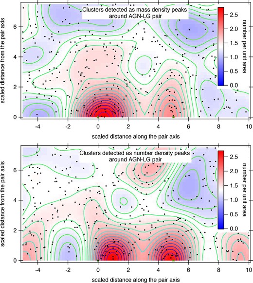
Distributions of clusters in the AGN–LG frame. The top panel is for clusters found as the stellar mass density peaks, and the bottom panel is for clusters found as the number density peaks. The x and y axes are scaled so that the the AGN and LG are located at (0,0) and (5,0), respectively. The contours of the number density are drawn in steps of 0.1 per unit area. (Color online)
In both plots, a concentration of clusters around the AGN located at (0,0) and around the LG at (5,0) is clearly seen. Looking at the positional distribution of the mass peak clusters (top panel of the figure), a weak feature elongated toward the vertical direction of the AGN–LG axis is indicated.
For the number peak cluster (bottom panel of the figure), the elongation is not clear at the LG position (x = 5) but is seen at the AGN position (x = 0). As a more outstanding feature, the peak of the concentration near the AGN is shifted toward the LG position.
To evaluate the significance of the anisotropy around the AGNs, we carried out a Monte Carlo simulation for the distribution of clusters in the AGN–LG frame. The simulation was conducted for each dataset of AGN–LG pairs by assuming the power law plus constant density distribution for clusters, as measured in the right panel of figure 16. The simulated positions of the clusters were converted into the AGN–LG frame according to the real positions of the AGN and LG. The ratios of the number count at the LG side (x = 0–2, y < 2) to the count at the anti-LG side (x = −2–0, y < 2) were then measured. These numbers for the real observation are 26 at the LG side and 11 at the anti-LG side, and thus the ratio is 0.70.
Among the 1000 sets of simulated samples, the maximum ratio was 0.61. Comparing this value with the real observed value of 0.70, the probability of obtaining the observed anisotropy was estimated to be less than 0.1%.
This anisotropy can be attributed to the overlap of clusters associated with the AGN and LG. Such an offset is not significant in the distribution of clusters detected as mass peaks, which may be due to a larger mass density for clusters associated with AGNs than clusters associated with LGs.
4.6 Peak density of clusters
To investigate the properties of the clusters associated with the target objects, we derived the distribution of peak densities for mass peak clusters and number peak clusters, in the same way as conducted for the color, absolute magnitude, and stellar mass described in the previous sections. In deriving the distributions, a high-density region was taken at <1 Mpc and a low-density region was considered at 2–6 Mpc.
The left panel of figure 18 shows the distribution of peak densities of the mass peak clusters, which demonstrates an excess of approximately σpeak = 1010.8–|$10^{11.6}\, M_{\odot }\:$|Mpc−2. The excess densities for the whole AGN and AGN–LG samples are larger than those for the blue galaxy sample at all peak densities. No significant difference is seen in the excess densities between the whole AGN and AGN–LG samples.
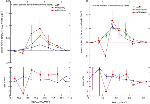
Left: Distributions of peak stellar mass density for three samples. The ratios to the densities measured for the whole AGN sample are plotted in the bottom panel. Right: As the left panel but for the peak number density. (Color online)
The right panel of figure 18 shows the distribution of peak densities of the number peak clusters. The excess densities for the whole AGN and blue galaxy samples are almost identical at below npeak < 101.8 Mpc−2. At higher peak densities, a decreasing trend is shown in the ratios of density for the blue galaxy to whole AGN. The excess densities for the AGN–LG sample are consistent with those of both the whole AGN and blue galaxy samples within the statistical error at >101.7 Mpc−2.
A depletion at 101.6–101.7 Mpc−2 for the AGN–LG sample can be seen, where no cluster was found at <1 Mpc whereas ∼5 clusters were expected. This may be due to the anisotropy of cluster distributions around the AGN of the AGN–LG pairs, as the position of the cluster is shifted toward the LG.
4.7 Number distribution of cluster
According to the results of the positional distribution of the clusters in the AGN–LG frame, multiple clusters that are associated with the AGN and LG are expected to exist in the environment near the AGN–LG pair. To test this, we compared the number distribution of clusters found within a 5 Mpc distance from the target objects. The distance scale of 5 Mpc was chosen to count clusters located within 1 Mpc of the LG, which is separated by 4 Mpc from the AGN at maximum. The thresholds of the peak density were set to 10|$^{11}\, M_{\odot }\:$|Mpc−2 and 101.8 Mpc−2 for the mass peak clusters and number peak clusters, respectively. These thresholds approximately correspond to the peak density of the distribution, as shown in figure 18.
Figure 19 shows the normalized distributions of the number of clusters for the three samples. The left panel is for the mass peak clusters and the right panel is for the number peak clusters. In both cases, there is no significant difference between the distributions for the AGN and blue galaxy samples, whereas the distributions for the AGN–LG sample are slightly shifted to a larger number.
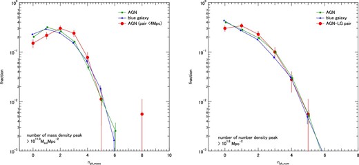
Left: Normalized distribution of number of clusters detected as stellar mass density peaks and found at <5 Mpc from the target objects. The threshold peak density was set to 10|$^{11}\, M_{\odot }\:$|Mpc−2. Right: The same plot for clusters detected as the number density peak. The threshold was set to 101.8 Mpc−2. (Color online)
The average numbers of clusters per field are plotted in figure 20 for the five samples, including AGN type 1 XR and AGN type 2 samples. We obtained 〈npeak, mass〉 (〈npeak, num〉) of 1.58 ± 0.03 (1.10 ± 0.03), 1.60 ± 0.03 (1.02 ± 0.03), 1.94 ± 0.12 (1.23 ± 0.09), 1.68 ± 0.06 (1.17 ± 0.05), and 1.55 ± 0.10 (1.13 ± 0.09) for the whole AGN, blue galaxy, AGN–LG pairs, AGN type 1 XR, and AGN type 2, where 〈npeak, mass〉 (〈npeak, num〉) represents the average number of mass peak clusters (number peak clusters).
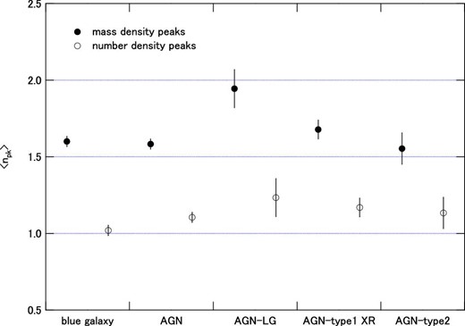
Average number of clusters found at <5 Mpc from the target objects. Solid circles represent the number for clusters detected as stellar mass density peaks and open circles represent the number for clusters detected as number density peaks.
The average number of mass peak clusters for the AGN–LG sample is 0.34 larger at ∼3 σ than that of the blue galaxy sample, whereas the difference in the average number of number peak clusters is small and less significant. No significant difference can be seen among the other samples, which is due to the dominance of the foreground and/or background clusters unassociated with the targets. These results indicate an environment in which the AGN–LG pairs have multiple clusters with higher probability than the others.
5 Discussion
5.1 Comparison of galaxy bias with other measurements
We measured the cross-correlation functions with the HSC sources, i.e., galaxies, for four types of AGN samples, i.e., whole AGNs with a mixture of any type, type 1 AGNs detected in the X-ray and/or radio band (AGN type 1 XR), type 2 AGNs, and AGN–LG pairs, as well as for a blue M* galaxy sample. For comparison with other observations, we derived a linear bias for galaxies clustering around those target objects. We did not attempt to derive the linear bias for AGN itself because of the difficulty arising from the dominance of the evolved galaxies, which were identified as a flat component in an absolute magnitude distribution, in the AGN fields.
From our previous study (Shirasaki et al. 2018), it is known that there is strong correlation between the AGN and LGs with magnitude brighter than M*, which is due to the evolution of M* into the luminous side for galaxies around the AGNs. In this study, we found that this evolution is related to the increase in the fraction of the secondary component in blue and red galaxies (referred to as a flat component collectively), as shown in figure 13. The dominance of the flat component makes it difficult to derive the absolute bias of the AGN from the cross-correlation with galaxies because we need to consider the clustering feature of the flat component. It is also inadequate to assume a simple linear relation between the AGN–galaxy cross-correlation function and auto-correlation functions of the AGN and galaxy, considering that the spatial distribution of the AGNs and the flat component are presumably not independent of each other.
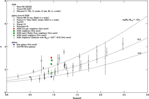
Conditional absolute biases measured for galaxies (Mλ310 < −19) around five target types: AGN–LG pair, AGN (all types), AGN type 1 XR (X-ray and/or radio detection), AGN type 2, and blue galaxies are plotted as solid makers. A bias calculated for galaxies with Mλ310 = −19.5–−18.5 around the AGN (all types) is also plotted with an open square. The same bias corresponding to our previous results (Shirasaki et al. 2018) and those obtained from the AGN–galaxy cross-correlation by other authors (Coil et al. 2007; Hickox et al. 2009, 2011; Zhang et al. 2013) are also shown. The absolute biases obtained for the AGN (Croom et al. 2005; Ross et al. 2009; Allevato et al. 2011) and galaxy (Coil et al. 2008) auto-correlation are also plotted. The dashed lines represent the redshift evolution of bias for a DM halo of the given mass, which is calculated in the same way as described in Shirasaki et al. (2018). (Color online)
In the same figure, the expected evolution in bias for DM haloes of different masses is also shown as a reference. We used the relation between the dark matter halo mass and the bias of the dark matter halo derived by Sheth, Mo, and Tormen (2001). As argued above, the conditional bias is affected by the evolution of galaxies around the AGNs, and should not be used as an estimator for the host DM halo mass. Thus, the large biases obtained for our three AGN samples (whole AGN, AGN type 1 XR, and AGN–LG pair) do not necessarily mean that they are hosted by DM haloes with |$>\!\!10^{13}\, M_{\odot }$|.
As a reference, we also calculated the conditional bias for galaxies with absolute magnitudes of Mλ310 = −19.5 to −18.5, where the contribution from the flat component becomes smaller (but not negligible), for the whole AGN sample. The corresponding cross-correlation length is ∼4.5 h−1 Mpc. This is shown in the same figure with an open square, and the bias comes close to that obtained from the AGN auto-correlation (Croom et al. 2005; Ross et al. 2009). If we assume the auto-correlation length of galaxies with those magnitudes to be ∼3.8 h−1 Mpc, which is the value obtained for galaxies around the blue galaxy sample, the auto-correlation length of the AGNs can be calculated as |$r_{\rm AA} = r_{\rm AG}^2/r_{\rm GG}$| ∼ 5.4 h−1 Mpc assuming the same power index of −1.8 of the correlation function. Then the bias is calculated as ∼1.9, which is consistent with those obtained by Croom et al. (2005) and Ross et al. (2009).
The conditional biases calculated from our previous results (Shirasaki et al. 2018) are also plotted in the same figure (solid black circles) for the z0 and z1 redshift groups. The bias obtained for the whole AGN sample in this work is consistent with the increasing trend at higher redshifts. The results obtained by Zhang et al. (2013), who adapted an analysis method similar to ours to the SDSS dataset, also show an increasing trend of the conditional biases.
The conditional bias measured for the AGN–LG sample is the largest of our samples, and is nearly the same as the one obtained for the AGN type 1 XR sample within the margin of error. The biases obtained for these two sub-types of AGNs are larger than that obtained for the whole AGN sample, which mostly consists of luminous type 1 AGN/QSO, by more than 3 σ.
The overdensity around AGNs with radio emission has been reported by numerous authors (e.g., Best et al. 2007; Hickox et al. 2009; Bradshaw et al. 2011). The clustering of X-ray selected AGNs is controversial. Coil et al. (2009) found that X-ray AGNs are more clustered than optically selected QSOs based on the cross-correlation with the same galaxy sample. In contrast, Krumpe et al. (2012) reported that there is no significant difference in the clustering of X-ray selected and optically selected broad-line AGNs. Thus, there seems to be a variety in the clustering of the X-ray selected AGNs, which is probably caused by the sample selection. The X-ray selected AGNs in our AGN type 1 XR sample are likely to reside in high-density environments, as the sample is dominated by X-ray selected AGNs as shown in table 3.
Our conditional bias for the blue galaxy sample is consistent with the bias obtained by Coil et al. (2008). In the case of this sample, the contribution from the flat component is almost negligible, and thus the bias obtained is expected to be close to the halo bias. The DM halo mass corresponding to the bias is |$M_{\rm h} \sim 10^{12}\, M_{\odot }$|.
We found a smaller cross-correlation length for the type 2 AGN sample than those for the other AGN samples, which is almost the same as that obtained for the blue galaxy sample. The clustering of type 2 AGNs drawn from the SDSS DR4 was examined by Li et al. (2006), who reported that no significant difference is shown between the type 2 AGNs and a reference sample of galaxies on scales of larger than a few Mpc. Allevato et al. (2011), by contrast, reported a similar bias parameter for both broad-line and narrow-line AGNs selected in the X-ray band. Their measurements of bias are plotted in figure 21, which shows a large bias for the narrow-line AGNs and a relatively smaller bias for X-ray obscured AGNs. Considering the large error bar, it is difficult to draw a conclusive answer to the difference in biases between the AGN types from their measurements.
Hickox et al. (2011) measured the cross-correlation with galaxies for obscured and unobscured QSOs. They argue that the obscured QSOs reside in a denser environment than the unobscured QSOs at the 1 σ level. More significant evidence has been obtained by recent works (e.g., DiPompeo et al. 2014, 2017), whereas other authors argue that there is no significant difference between the environments of obscured and unobscured (or type 1 and type 2) QSOs (e.g., Mendez et al. 2016). Based on clustering analysis for AGNs in the local Universe, several authors have reported that obscured AGNs (or type 2 AGNs) reside in denser environments than unobscured (or type 1 AGNs; see, e.g., Jiang et al. 2016; Powell et al. 2018; Krumpe et al. 2018) if it is measured at small scales (<1 Mpc). Based on the HSC-SSP dataset, Toba et al. (2017) measured the clustering properties of infrared bright dust-obscured galaxies (DOGs), which is thought to be powered by active star formation and/or an AGN hidden by surrounding dust, and they report large bias for those populations.
For comparison with our results, conditional biases calculated from the cross-correlation lengths obtained by Hickox et al. (2011) for obscured and unobscured QSOs are plotted in figure 21. Their biases are significantly smaller than our previous result obtained for whole AGNs at z = 1.2 and the extrapolation of this work for whole AGNs along the bias evolution for the same halo mass, whereas the extrapolation of this work for type 2 AGNs is almost consistent with their results. Coil et al. (2009) also reported a smaller bias for the AGN sample as compared to our result for the whole AGN sample at a redshift of ∼1. The calculated conditional bias for the AGN sample of Coil et al. (2009) is almost the same as the bias obtained for a blue galaxy in Coil et al. (2008).
It is possible that the inconsistency between their results and ours comes from the difference in the estimation of the average number density of the correlated galaxies. In our analysis the galaxy density is estimated from the model of the luminosity function, which was derived from the luminosity functions obtained by several deep surveys. Because the statistics are usually low for galaxies at the luminous end of the luminosity function derived from deep surveys, the flattening of the luminosity function at <M* owing to the emergence of the flat component, as observed in this study, could be completely missed.
This leads our analysis to an underestimation of the average number density of galaxies, which results in a higher cross-correlation with bright galaxies. In the studies by Hickox et al. (2011) and Coil et al. (2007), the average number density was estimated from the galaxy sample itself, and the sample usually had sufficient statistics for detecting a flat component. Despite the possible uncertainty in the estimation of the average number density in our analysis, it is expected to be small considering the consistency found for a blue galaxy sample between ours and Coil et al. (2008). Thus, the inconsistency could be due to the difference in the sample selection for the AGNs and/or galaxies.
Although there is difficulty in comparing with other works carried out using different methods and samples, a reliable comparison is possible if it is made under the same method and same galaxy sample. The differences found between our different target samples are more reliable, because they were compared under the same conditions to the greatest extent possible. In the next section we discuss the properties of the environment around AGN–LG pairs based on the results derived from fair comparisons.
5.2 Properties of the environment around AGN–LG pairs
As discussed in the previous section, the environment around AGN–LG pairs is characterized as a high-density region if compared in a high luminosity range (M < M*). The projected cross-correlation function is as large as that of AGNs with radio and/or X-ray emission, which have been known to be located in higher-density regions compared to the other type of AGNs. As shown in figure 4, the luminosity of the AGNs in the AGN–LG pair sample is relatively lower than those in the whole AGN sample. One possible reason for this is that the AGNs in the AGN–LG pair sample are dominated by AGNs obscured by their surrounding dust to a certain degree. There have been several studies suggesting that obscured AGNs tend to reside in denser regions than unobscured AGNs (e.g., Hickox et al. 2011; DiPompeo et al. 2014, 2017; Powell et al. 2018). Another possibility is the contribution of intrinsically less luminous AGNs, which are driven by, e.g., a quiescent accretion of hot halo gas (Kereš et al. 2009; Fanidakis et al. 2013).
We also found an excess in the average number of mass peak clusters for the AGN–LG sample (figure 20) against those measured for the other samples. In addition to this, we also found that the positional distribution of the number peak clusters departs from an isotropic distribution around each AGN and LG when they are measured in the AGN–LG pair frame (bottom panel of figure 17). These results indicate that, for a portion of the AGN–LG pairs, at least two clusters are located around them.
The luminosity function of blue galaxies at distances of less than 2 Mpc from the AGNs of the AGN–LG pairs was measured, and it can be better expressed with a linear combination of two Schechter functions with different M* and α values, as shown in figure 13. The component characterized with a larger (fainter) M* (primary component) is a main component at magnitudes fainter than Mλ310 = −19 mag. The other component (secondary component), which dominates at magnitudes brighter than Mλ310 = −20 mag, is characterized with a smaller (brighter) M* and a flat slope parameter of α ∼ 0.
The luminosity function of red galaxies was also measured, and it is likely to have similar characteristics to the secondary component found in the luminosity function of the blue galaxies. Thus, both components are presumably produced by a common mechanism, and we refer to them as a flat component hereafter. The same features are also found for galaxies in the other two samples, i.e., whole AGN and blue galaxy samples.
Comparing the ratios of the number density of the secondary component of blue galaxies φB2 to that of the primary component φB1 (table 10), they are almost the same (0.078 ± 0.014 for whole AGN and 0.075 ± 0.023 for AGN–LG pairs), whereas the fraction for the blue galaxy (0.021 ± 0.018) is significantly smaller than that of the other two samples.
The comparison of the stellar mass distributions around the targets among the three samples shows flatter distributions at larger stellar masses for the AGN and AGN–LG samples than for the blue galaxy sample (figure 15). This can be explained by the higher fraction of the flat component, which are typically luminous and thus have a larger stellar mass, for the AGN and AGN–LG samples.
These results indicate that some type of AGN preferentially occurs in an environment in which galaxies are rapidly evolving toward a red sequence. The flat component of blue galaxies could be the intermediate state of a galaxy evolving toward a red sequence galaxy considering the similarity between the luminosity functions.
We were unable to find any significant difference in the properties of clusters for the AGN and AGN–LG pair samples within the immediate environment of <1 Mpc from the AGNs. The clustering of clusters around the AGN is nearly the same for both samples (figure 16), and the distributions of peak density of the mass peak clusters and number peak clusters are also identical within the statistical error (figure 18). A difference is seen if they are compared at a larger scale.
For the AGN–LG sample, we found that the average number of mass peak clusters at <5 Mpc from the AGNs is larger than those for the other samples (figure 20), which indicates that the large clustering of LGs, i.e., the emergence of a flat component for the AGN–LG pairs, is related to the larger clustering of DM haloes at a scale of several Mpc. For the AGN type 1 XR sample, by contrast, we were unable to find a significant difference in the number of mass peak clusters from the other samples, i.e., whole AGN, blue galaxy, and AGN type 2 samples. This might be explained as two clusters being located too close to be identified as separate mass peak clusters or already merged into a single large cluster in the environment of AGN type 1 XR. At any rate, the existence of multiple clusters around AGN–LG pairs indicates that there is some cluster-scale mechanism invoking AGN activity and evolution of surrounding galaxies simultaneously.
There is an argument that LGs are known to be highly clustered, thus the environment of the AGN–LG pairs consequently should be a high-density region and have higher probability of association of nearby clusters. This argument, however, is not adequate in explaining why there is a large cross-correlation between AGN and LG seperated by several Mpc, which is the original question raised at the start of this work. We argue, instead, that the large-scale interaction of clusters could be a primary driver for producing AGNs and luminous galaxies in the restricted regions, which leads to the strong cross-correlation between them. Our observational results support this argument.
6 Summary and conclusion
We have investigated the properties of the environment around AGN and luminous galaxy pairs (AGN–LG pairs) to understand what causes the strong correlation between AGNs and LGs found in Shirasaki et al. (2018). From a comparison of the environmental properties measured for four AGN samples, (whole AGN, AGN–LG, AGN type 1 XR, and AGN type 2 samples) and one blue galaxy sample, the following information was obtained:
AGNs are preferentially located in an environment where luminous galaxies (M < M*) are enriched compared to the environment of blue M* galaxies. The measured cross-correlation lengths with galaxies (Mλ310 < −19) are 7.22 ± 0.16 h−1 Mpc and 3.77 ± 0.27 h−1 Mpc for the whole AGN and blue galaxy samples, respectively. All cross-correlation lengths are calculated for γ = 1.8.
The environment of type 2 AGNs is similar to that of blue M* galaxies. The measured cross-correlation length is 4.77 ± 0.78 h−1 Mpc for the AGN type 2 sample.
The luminosity of the AGNs in the AGN–LG sample is typically lower than that of the whole AGN sample, which may indicate that they are dominated by obscured and/or intrinsically less luminous AGNs.
AGNs in the AGN–LG sample are located in an environment of slightly higher density than those in the whole AGN sample. The measured cross-correlation length is 9.03 ± 0.44 h−1 Mpc for the AGN–LG sample. The cross-correlation is almost equivalent to that obtained for the AGN type 1 (RX) sample, which is 8.27 ± 0.31 h−1 Mpc.
The cross-correlation length of AGNs with fainter galaxies comes close to that measured for blue galaxies. This indicates that the mass of the dark matter halo hosting AGNs is not particularly high, but is at most a few times as large as that of the hosting blue galaxies.
The luminosity functions around the AGNs and blue galaxies are expressed by a linear combination of two Schechter functions: one represents the primary component at the faint end M > M*, and the other one represents a flat component characterized by a flat slope parameter (α ∼ 0) and brighter M* than that of the primary component.
The ratio of the flat component to the primary component measured at Mλ310 = −18 is three times higher in an AGN environment than in a blue galaxy environment. The larger cross-correlation lengths obtained for the AGN samples are mostly due to enhancement of the flat component.
As expected from the enhancement of the flat component, which is characterized by bright, and hence a large, stellar mass, an enrichment of large stellar mass galaxies was measured around the AGNs as compared to around the blue galaxies.
The clustering of clusters detected as stellar mass density peaks (mass peak clusters) is larger around the AGNs than around the blue galaxies, whereas the clustering of clusters detected as the number density peaks (number peak clusters) is almost the same between them. No statistically significant difference is shown between the whole AGN and AGN–LG samples.
The clustering of the mass peak cluster around the AGNs is almost equally larger at any peak density of clusters than that around the blue galaxies. The clustering of number peak clusters around the AGNs is similar for a smaller peak density (<101.8 Mpc−2), and becomes larger at a larger peak density (≥101.8 Mpc−2). No statistically significant difference is shown between the whole AGN and AGN–LG samples.
The anisotropic distribution of clusters was found in an environment of AGN–LG pairs if measured in the AGN–LG frame. We found that the peak position of the number peak clusters near the AGNs is shifted toward the LG direction, which indicates the coexistence of two clusters around the AGN–LG pairs.
An excess average number of mass peak clusters was found for the AGN–LG sample against the other samples, which again indicates enhancement of the number of clusters in the AGN–LG pair environments.
Based on these findings, the following scenario regarding the evolution of an AGN and a galaxy can be drawn: AGNs, at least some classes of AGNs, are preferentially produced in an environment in which the number density of dark matter haloes is relatively high. In such an environment, star formation is ignited in multiple galaxies by a large-scale mechanism related to the multiple dark matter haloes, and then evolves through green valley galaxies with quenched star formation, finally becoming red sequence galaxies. An AGN is an episodic event produced along with galaxy evolution, and thus the strong correlation of an AGN and luminous galaxies is a natural consequence in such an environment. Collisions and/or interaction of dark matter haloes is a possible mechanism facilitating such galaxy evolution at a large scale.
Acknowledgements
We would like to thank the anonymous referee for the constructive feedback, which helped us in improving the paper.
This work is based on data collected at the Subaru Telescope and retrieved from the HSC data archive system, which is operated by Subaru Telescope and Astronomy Data Center, National Astronomical Observatory of Japan. The Hyper Suprime-Cam (HSC) collaboration includes the astronomical communities of Japan and Taiwan, and Princeton University. The HSC instrumentation and software were developed by the National Astronomical Observatory of Japan (NAOJ), the Kavli Institute for the Physics and Mathematics of the Universe (Kavli IPMU), the University of Tokyo, the High Energy Accelerator Research Organization (KEK), the Academia Sinica Institute for Astronomy and Astrophysics in Taiwan (ASIAA), and Princeton University. Funding was contributed by the FIRST program from the Japanese Cabinet Office, the Ministry of Education, Culture, Sports, Science and Technology (MEXT), the Japan Society for the Promotion of Science (JSPS), the Japan Science and Technology Agency (JST), the Toray Science Foundation, NAOJ, Kavli IPMU, KEK, ASIAA, and Princeton University.
This paper makes use of software developed for the Large Synoptic Survey Telescope. We thank the LSST Project for making their code available as free software at 〈http://dm.lsstorp.org〉.
The Pan-STARRS1 Surveys (PS1) have been made possible through contributions of the Institute for Astronomy, the University of Hawaii, the Pan-STARRS Project Office, the Max-Planck Society and its participating institutes, the Max Planck Institute for Astronomy, Heidelberg and the Max Planck Institute for Extraterrestrial Physics, Garching, The Johns Hopkins University, Durham University, the University of Edinburgh, Queen’s University Belfast, the Harvard-Smithsonian Center for Astrophysics, the Las Cumbres Observatory Global Telescope Network Incorporated, the National Central University of Taiwan, the Space Telescope Science Institute, the National Aeronautics and Space Administration under Grant No. NNX08AR22G issued through the Planetary Science Division of the NASA Science Mission Directorate, the National Science Foundation under Grant No. AST-1238877, the University of Maryland, and Eotvos Lorand University (ELTE) and the Los Alamos National Laboratory.
Funding for the Sloan Digital Sky Survey IV has been provided by the Alfred P. Sloan Foundation, the U.S. Department of Energy Office of Science, and the Participating Institutions. SDSS-IV acknowledges support and resources from the Center for High-Performance Computing at the University of Utah. The SDSS web site is 〈www.sdss.org〉. SDSS-IV is managed by the Astrophysical Research Consortium for the Participating Institutions of the SDSS Collaboration including the Brazilian Participation Group, the Carnegie Institution for Science, Carnegie Mellon University, the Chilean Participation Group, the French Participation Group, Harvard-Smithsonian Center for Astrophysics, Instituto de Astrofísica de Canarias, The Johns Hopkins University, Kavli Institute for the Physics and Mathematics of the Universe (IPMU) / University of Tokyo, Lawrence Berkeley National Laboratory, Leibniz Institut für Astrophysik Potsdam (AIP), Max-Planck-Institut für Astronomie (MPIA Heidelberg), Max-Planck-Institut für Astrophysik (MPA Garching), Max-Planck-Institut für Extraterrestrische Physik (MPE), National Astronomical Observatories of China, New Mexico State University, New York University, University of Notre Dame, Observatário Nacional / MCTI, The Ohio State University, Pennsylvania State University, Shanghai Astronomical Observatory, United Kingdom Participation Group, Universidad Nacional Autónoma de México, University of Arizona, University of Colorado Boulder, University of Oxford, University of Portsmouth, University of Utah, University of Virginia, University of Washington, University of Wisconsin, Vanderbilt University, and Yale University.
Funding for the DEEP2 Galaxy Redshift Survey has been provided by NSF grants AST-95-09298, AST-0071048, AST-0507428, and AST-0507483, as well as NASA LTSA grant NNG04GC89G.
This research uses data from the VIMOS VLT Deep Survey, obtained from the VVDS database operated by Cesam, Laboratoire d’Astrophysique de Marseille, France.
This paper uses data from the VIMOS Public Extragalactic Redshift Survey (VIPERS). VIPERS has been performed using the ESO Very Large Telescope, under the “Large Programme” 182.A-0886. The participating institutions and funding agencies are listed at 〈http://vipers.inaf.it〉.
Funding for PRIMUS is provided by NSF (AST-0607701, AST-0908246, AST-0908442, AST-0908354) and NASA (Spitzer-1356708, 08-ADP08-0019, NNX09AC95G). This research has made use of NASA’s Astrophysics Data System. This research has made use of the VO service toolkit developed by the Japanese Virtual Observatory group at ADC, NAOJ. We would like to thank the members of HSC AGN WG for a fruitful discussion. We would like to thank Editage 〈http://www.editage.com〉 for editing the first version of the manuscript for English language.
References
