


Abstract
Complete studies of the radiative processes of thermal emission from the amorphous dust from microwave through far-infrared wavebands are presented by taking into account, self-consistently for the first time, the standard two-level systems (TLS) model of amorphous materials. The observed spectral energy distributions (SEDs) for the Perseus molecular cloud (MC) and W 43 from microwave through far-infrared are fitted with the SEDs calculated with the TLS model of amorphous silicate. We have found that the model SEDs reproduce the observed properties of the anomalous microwave emission (AME) well. The present result suggests an alternative interpretation for the AME being carried by the resonance emission of the TLS of amorphous materials without introducing new species. Simultaneous fitting of the intensity and polarization SEDs for the Perseus MC and W 43 are also performed. The amorphous model reproduces the overall observed feature of the intensity and polarization SEDs of the Perseus MC and W 43. However, the model’s predicted polarization fraction of the AME is slightly higher than the QUIJOTE upper limits in several frequency bands. A possible improvement of our model to resolve this problem is proposed. Our model predicts that interstellar dust is amorphous materials with very different physical characteristics compared with terrestrial amorphous materials.
1 Introduction
Studies of the physical processes of thermal emission from Galactic dust have been a long-standing problem and are still of significance. The typical temperature of Galactic interstellar dust is about 20 K (Schlegel et al. 1998; Planck Collaboration 2014). Its emission appears predominantly at long wavelengths from the far-infrared through microwave. Since the whole sky is covered by the emission from Galactic interstellar dust, thermal emission from the Galactic dust is a serious obstacle for the detection of B-mode polarization signals from cosmic microwave background (CMB) radiation imprinted by primordial gravitational waves. The success of CMB B-mode polarization observations relies on how accurately we can remove the Galactic dust signals from observational data. To tackle this difficult task, many CMB experiments are under way and others are being planned (e.g., ACTPol: Naess et al. 2014; BICEP2/3 and the Keck Array: Grayson et al. 2016; CLASS: Essinger-Hileman et al. 2014; GroundBIRD: Oguri et al. 2016; LiteBIRD: Matsumura et al. 2014; PIPER: Gandilo et al. 2016; POLARBEAR and the Simons Array: Arnold et al. 2014; QUIJOTE: Rubiño-Martín et al. 2012; the Simons Observatory: Ade et al. 2019; SPIDER: Gualtieri et al. 2018; SPTPol: Austermann et al. 2012). These surveys provide extremely high precision data on the microwave sky with wide sky coverage in many different wavebands. It is certain that significant progress in our understanding of interstellar dust will be made with these data. Therefore, theoretical studies of the physical processes of thermal emission from Galactic dust must be undertaken now to achieve fruitful outcomes from these data.
The origin of anomalous microwave emission, which is abbreviated as AME, found ubiquitously in the Galaxy at around 10–30 GHz [e.g., see Dickinson (2013) for a summary of AME observations in H ii regions] is still under debate. The spatial correlation between AME and Galactic interstellar dust strongly indicates that AME originates from a kind of dust (Davies et al. 2006). The most popular model of the origin of AME is electric dipole emission radiated by charged rotating dust with a frequency of several tens of GHz, as proposed by Draine and Lazarian (1998); this is referred to as the spinning dust model. A carrier of the spinning dust is supposed to be very small grains producing rotation at ultra-high frequencies. The fact of the lack of AME in cold dense cores supports the spinning dust origin of AME since the lack of small grains is expected in dense clouds (Tibbs et al. 2016). Polycyclic aromatic hydrocarbon (PAH) has been proposed as one of the plausible candidates for spinning dust (Draine & Lazarian 1998). However, the lack of observational correlation between the amount of PAH and the intensity of AME, as reported by Hensley et al. (2016), contradicts the PAH possibility. A new species of very small dust grains named nanosilicates has been introduced as another possible carrier of the spinning dust (Hoang et al. 2016; Hensley & Draine 2017). The problem with this possibility is that up to now, apart from AME, no signature to confirm the existence of the nanosilicate has been observed. The nanosilicate is only observable as AME. Therefore, it is hard to check whether the carrier of the spinning dust is such a new family of dust grains or not.
Magnetic dust emission has been proposed as another candidate for the AME mechanism (Draine & Lazarian 1999). The spins of electrons inside a magnetic dust grain align spontaneously to settle down to the minimum energy state. Alignment is disturbed by thermal fluctuation. Owing to the magnetic relaxation, the disturbed state tries to return to the original minimum energy state. In course of this transition, microwave radiation is emitted. This emission could be the origin of AME if the interstellar dust is magnetic (Draine & Hensley 2013). The magnetic dust emission model predicts a positive correlation between the temperature and intensity of AME. However, Hensley et al. (2016) found a negative correlation between the AME temperature and intensity that contradicts the predictions of the magnetic dust emission model. A comprehensive review of the state of AME research is given by Dickinson et al. (2018).
A crucial clue to distinguishing the emission mechanisms of AME is offered by polarization observations. Draine and Hensley (2016) showed that the quantum effect suppresses the thermalization of the grain rotational kinetic energy of the spinning dust. As a result, the alignment of grains is suppressed and the spinning dust model predicts a very low degree of polarization. In the magnetic dust emission model, a high degree of AME polarization is expected since the main carriers of magnetic dust emission are large grains which are aligned by the interstellar magnetic field. Although the progress of AME polarization observations have been made by several projects (e.g., WMAP and QUIJOTE), there has as yet been no definite report of the detection of AME polarization (Génova-Santos et al. 2015, 2017). The detection of polarization from AME has been reported for W 43, but whether the reported polarization is a residual of the synchrotron emission of Galactic interstellar matters around W 43 is still being debated. Current observational upper limits somehow rule out the magnetic dust hypothesis, which typically predicts a higher polarization fraction.
Almost all types of interstellar dust are supposed to be made of amorphous materials. For example, the broad emission line observed ubiquitously in interstellar space at |$9.7\, \mu \mathrm{m}$| is considered to be a signature that one of the main components of interstellar dust is an amorphous silicate (Kraetschmer & Huffman 1979; Li & Draine 2001). Moreover, laboratory simulations of cosmic dust analogues suggest that various forms of amorphous carbon grains are more favorable than graphite grains (Colangeli et al. 1995; Zubko et al. 1996). The observed spectrum of interstellar dust emission in submillimeter wavebands obtained by the Planck satellite is flatter than the spectrum expected from crystal dust (Planck Collaboration 2014). This is further evidence indicating that interstellar dust is composed of amorphous dust. According to recent laboratory measurements of the emissivity of amorphous material, the emissivity of the amorphous material has complex frequency dependences that cannot be approximated by a single power-law at longer than far-infrared wavelengths (e.g., Coupeaud et al. 2011). Physical diagnostics of the amorphous material appear in heat capacity and heat conductivity at very low temperature. Zeller and Pohl (1971) found that the heat capacity of the amorphous material below 1 K shows significant deviation from the Debye model and depends linearly on temperature instead of the cube of the temperature. They also found that heat conductivity below 1 K is in excess of that expected for crystals and depends on the square of the temperature. It has also been shown that these characteristics appear universally in any amorphous material. This universality indicates that above-mentioned diagnostics observed in amorphous materials are governed by universal physics. Anderson, Halperin, and Varma (1972) and Phillips (1972) independently proposed that heat absorption and heat transport by two-level systems from amorphous materials predominate over lattice oscillation below 1 K. This model is referred to as the TLS model. The degree of freedom concerning heat absorption becomes one when absorption by the TLS becomes dominant below 1 K. That is why the temperature dependence of the heat capacity switches from cubic to linear. The temperature dependence of the heat conductivity below 1 K is also successfully explained by the TLS model. Agladze et al. (1994) showed that the temperature dependence of the absorption coefficient in far-infrared wavebands measured for amorphous powder are well described by the TLS model in laboratory experiments. They were the first to propose that the TLS may contribute to the observed features of interstellar dust. Meny et al. (2007) performed theoretical calculations of the frequency dependence of the absorption coefficient based on the TLS model. Paradis et al. (2011) compared their models with the observed spectra of diffuse interstellar dust from far-infrared through submillimeter wavebands. They showed that the TLS model succeeds in reproducing the observed features, including the inverse correlation of the spectral index with dust temperature.
Jones (2009) proposed the idea that the AME might originate from the resonance emission due to radiative transition between the TLS of amorphous dust. The fact that the effect of the TLS appears below 1 K indicates that the energy splitting between the TLS is about |$10^{-4}\:$|eV, which just coincides with the observed frequency of the AME. Therefore, the resonance emission from amorphous dust is an attractive possibility for the origin of AME. The negative correlation between the AME temperature and intensity is naturally explained by the amorphous model since the intensity of the resonance emission decreases as the dust temperature increases (Meny et al. 2007). They assumed that the peak value of the absorption cross-section of the resonance process of the TLS is the geometric cross-section. It is well known, however, that the absorption cross-section of a small particle at microwave wavelengths is much smaller than the geometric cross-section (e.g., Draine & Lee 1984). It is likely that their model overestimates the TLS contribution. It is also still unclear what kind of physical characteristics of the amorphous dust can be extracted from the observation of AME. Because of the potential possibility of the amorphous origin of AME, studies of the thermal emission of amorphous dust relying on microscopic physical processes based on the TLS model are required.
In this paper, the intensity and polarization spectral energy distributions (SEDs) modeling from far-infrared through microwave wavelengths are conducted based on the TLS model of amorphous dust. By comparing the model with observations, we study whether the amorphous dust model is able to explain the diagnostics of the entire frequency range spectrum; e.g., the emission peak in the far-infrared, the spectral index in submillimeter wavebands, the bump in the emission of the AME, and the low polarization fraction of the AME. We show what kind of physical characteristics are required for the amorphous dust in order to explain the observations. We adopt two archetypical AME objects, the Perseus molecular cloud (MC) and W 43, for our comparison with the observations. Both objects have intensive data on the intensity and polarization spectrum over a wide number of frequency bands.
In section 2, fundamental quantities of amorphous materials to describe their optical properties are summarized. (Details of the basics of the standard TLS model are introduced in appendix 1.) In section 3, we show how the SEDs of the thermal emission from amorphous silicate dust respond to the physical parameters of the TLS model and compare model SEDs with observational data. We then move on to the polarized emission in section 4. In section 5, we examine the properties of the amorphous silicate dust. Limitations of the present model and possible improvements are discussed in section 6. Our conclusions and a summary are presented in section 7.
2 Summary of fundamental quantities of amorphous materials to describe their optical properties
Optical properties of an amorphous material are determined by its electric susceptibility (see the details in sections 3 and 4). In this section, we summarize how the electric susceptibilities due to the TLS and disordered charged distribution (DCD) are related to the micro-physics of each process, respectively. The details of the standard TLS model are described in appendix 1. The basic equations of the TLS model and the DCD model can apply to both amorphous silicate material and amorphous carbon material since the physical mechanism behind each model does not depend on the material composition. The differences between the amorphous silicate material and the amorphous carbon material appear in the differences of values of physical variables.
2.1 TLS model
The basic idea of the TLS model is that some of the atoms composing an amorphous material have two stable positions due to deformation of crystal structures. The mechanical potential of the atom is described by the double-well potential illustrated in figure 1. The |$x$|-coordinate marks the position of the atom. This potential is generally described by a quartic function of |$x$|, which is called the soft-potential model (Karpov et al. 1982). In this paper, in order to describe how the TLS modifies the spectrum of the thermal emission from dust and determine whether AME can be explained by introducing the TLS model, we adopt the same approximation made by Anderson, Halperin, and Varma (1972) and Phillips (1972), who first proposed the TLS model to describe the physical characteristics of the amorphous materials appearing at very low temperature. They expanded the ground state and the first excited state of the Schrödinger equation of the atom confined in the double-well potential |$V$| by the two ground states when the atom is confined in each harmonic potential |$V_1$| and |$V_2$| individually (see figure 1). We refer to this model as the standard TLS model.
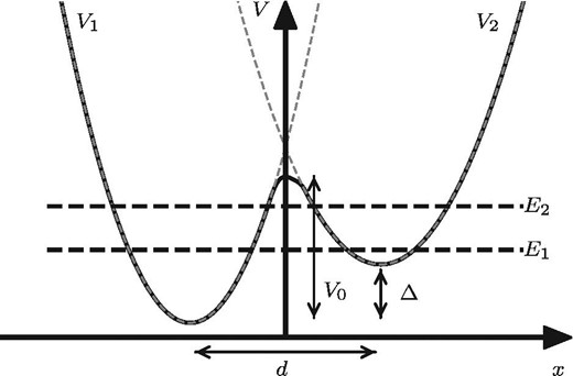
Double-well potential, shown by the black solid curve, in which an atom is trapped. The gray dashed curves denote harmonic potentials |$V_1$| and |$V_2$|.
2.2 Disordered charged distribution model
Typical values of physical variables of an amorphous silicate material.
| Parameter | Meaning | Value | Unit | Ref.|$\ddagger$| |
|---|---|---|---|---|
| |$V_m / k_\mathrm{B}$| | Mean value of the barrier height distribution | 550 | K | 1 |
| |$V_\sigma / k_\mathrm{B}$| | Deviation of the barrier height distribution | 410 | K | 1 |
| |$V_\mathrm{min} / k_\mathrm{B}$| | Lower cutoff of the barrier height distribution | 50 | K | 1 |
| |$\rho$| | Mass density of a dust particle | 3.5 | g cm|$^{-3}$| | 2 |
| |$n_\mathrm{atom}$| | The number density of atoms composing a dust particle | |$\rho /172.2 \times 7 N_\mathrm{A}$|* | cm|$^{-3}$| | 2 |
| |$c_\mathrm{t}$| | Sound velocity for transverse waves | |$3 \times 10^5$| | cm s|$^{-1}$| | 1 |
| |$\gamma _\mathrm{t}$| | Elastic dipole for transverse waves | 1 | eV | 3 |
| |$|\boldsymbol {d}_0|$| | Electric dipole moment for the localized state at the bottom of |$V_2$| | 1 | D | 1 |
| |$\tau _\mathrm{hop}^0$| | Pre-exponential factor for hopping relaxation time [see equation (A52)] | 10|$^{-13}$| | s | 1 |
| |$l_\mathrm{c}$| | Correlation length of propagation of lattice vibration | 30 | Å | 1 |
| |$q^2$| | Electric charge of an atom composing a dust particle | |$e^2$| | erg cm | 2 |
| |$m$| | Mass of an atom composing a dust particle | |$m_\mathrm{O}$| † | g | 2 |
| |$\omega _\mathrm{D}$| | Debye angular frequency | |$2 \pi c_\mathrm{t} [9 n_\mathrm{atom} / (8 \pi )]^{1/3}$| | s|$^{-1}$| | — |
| |$C$| | Correction factor for the DCD model | |$4.15 \times 10^{-2}$| | — | — |
*|$N_\mathrm{A}$| is the Avogadro constant and we consider the composition of amorphous silicate materials as |$\mathrm{MgFeSiO_4}$|, the mass number of which is |$172.2\:$|g|$\:$|mol|$^{-1}$|.
|$^{\dagger }$| |$m_\mathrm{O}$| is the mass of an oxygen atom.
3 Thermal emission from amorphous silicate dust
3.1 Absorption cross-section
3.2 Intensity emission spectra of thermal emission
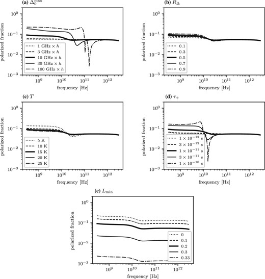
Figure 2 shows the parameter dependence of thermal emission SEDs from amorphous silicate dust. The results show that the bump emission appears at around several tens of GHz. This is caused by the resonance transition of the TLS. Figure 2a shows that the peak frequency of the bump emission is shifted toward higher frequency as the upper limit of the energy difference between the TLS, |$\Delta _0^\mathrm{max}$|, increases while |$R_\Delta$| (|$\equiv \Delta _0^\mathrm{min}/\Delta _0^\mathrm{max}$|) is fixed. Figure 2b shows that the bump feature of the resonance emission becomes broader as |$R_\Delta$| gets smaller, although the response is not prominent. Figure 2c shows that the bump emission due to the resonance process relative to the far-infrared peak becomes higher when the temperature of the dust grain lowers. This is attributed to the fact that the electric dipole moment caused by the resonance transition rate increases with decreasing temperature because the fraction of atoms in the ground state increases with decreasing temperature [see appendix 1, equation (A46)]. Figure 2d shows that the width of the bump emission sensitively responds to the relaxation time scale of the resonance process, |$\tau _+$|. Figures 2a and 2b show that the bump emission becomes prominent when |$1/\tau _+$| becomes comparable to, or greater than, |$\Delta _0^\mathrm{max} / h$|. Figure 2e shows that the peak intensity of the bump emission caused by the resonance process is about two orders of magnitude lower than the peak intensity in the far-infrared, even when all the atoms are trapped in the TLS. The relative intensity of the bump emission decreases almost linearly with |$f_\mathrm{TLS}$|.
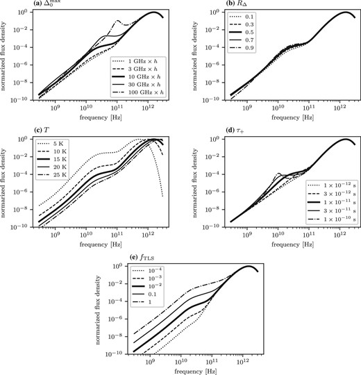
Parameter dependences of the SEDs of dust thermal emission in the standard TLS model. SEDs are given in arbitrary units normalized to each maximum value. Thick solid curves in each panel show the SEDs with the same parameter values. In each panel, one of the variables characterizing the amorphous silicate dust was varied to see how the shape of the SED responds for each variable. The variables are (a) |$\Delta _0^\mathrm{max}$| which are expressed in the corresponding frequency normalized by the Planck constant |$h$|, (b) |$R_{\Delta }$|, (c) |$T$|, (d) |$\tau _+$|, and (e) |$f_\mathrm{TLS}$|, respectively. Given values for each parameter are shown in legends.
To clarify how the frequency dependence of the thermal emission of amorphous silicate dust is defined, figure 3 shows SEDs for each process. The frequency dependence of the absorption coefficient of the resonance process and the relaxation processes in submillimeter wavebands are described by |$C_\nu ^\mathrm{res} \propto \nu ^2$| and |$C_\nu ^\mathrm{rel} \propto \nu$|, respectively. The frequency dependence of the resonance process in the long wavelength limit is the same as for crystal. As the wavelength increases starting from the far-infrared, the contributions from tunneling and hopping relaxation become more significant. As a result, the slope of the absorption coefficient of the amorphous material becomes flatter than that of crystal in the submillimeter wavelength range.
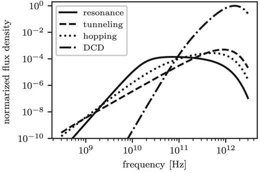
Dust thermal emission SEDs caused by each TLS and DCD process. Parameters have the same values as the thick solid curves in figure 2. Every curve is normalized to the peak value of the SED arising from the DCD.
3.3 Comparison with observed spectra
3.3.1 Intensity SED data and modeling
where |$T_\mathrm{CMB} = 2.725\:$|K (Mather et al. 1999) is the CMB temperature.
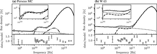
Spectra of two archetypal dust-rich objects accompanying prominent AME, (a) the Perseus MC and (b) W 43, are fitted by our amorphous model. Dashed curves are the best-fitting thermal emission model from amorphous silicate dust, and dotted lines are the best-fitting free–free emission contribution. In both sets of data, contributions from the Galactic interstellar medium are subtracted. Although temperature fluctuation of the CMB is subtracted from the spectrum of W 43, it is not taken into account in the spectrum of the Perseus MC. Therefore, the CMB contribution is taken into account in the SED fit for the Perseus MC. As shown in table 2, the best CMB temperature fluctuation takes a negative value. The absolute value of the best-fitting CMB contribution is shown by dash–dotted line in panel (a). The solid curves show the total SEDs of the best-fitting models. The bottom panel inserted in each figure shows the data-to-model ratio.
Best-fitting parameters for the Perseus MC and W 43.*
| Perseus MC | W 43 | ||
|---|---|---|---|
| without | with CMB | ||
| |$T$| (K) | 16.78 ± 0.08 | 16.90 ± 0.08 | 20.20 ± 0.06 |
| |$\tau _{250}\ (\times 10^{-4})$| | 4.08 ± 0.08 | 3.87±0.07 | 58.3±0.5 |
| |$f_\mathrm{TLS}$| | 0.0123±0.0003 | 0.0151±0.0004 | 0.0338±0.0004 |
| |$\Delta _0^\mathrm{max}/h$|(GHz) | 15.2±0.2 | 15.0±0.2 | 11.0±0.1 |
| |$R_\Delta$| | 0.716±0.023 | 0.648±0.022 | 0.927±0.006 |
| |$\tau _+ \ (\times 10^{-11}\:\mbox{s})$| | 2.24±0.09 | |$2.19^{+0.09}_{-0.08}$| | 2.89±0.05 |
| EM (cm|$^{-6}\:$|pc) | 26.9±2.4 | 26.7±2.4 | 3934±29 |
| |$\Delta T_\mathrm{CMB} \ (\mu \mbox{K})$| | — | |$-19.3^{+6.3}_{-5.9}$| | — |
| dof | 21 | 18 | 23 |
| |$\chi ^2/\mathrm{dof}$| | 2.04 | 1.67 | 6.41 |
*The errors are at |$1\sigma$|.
Best-fitting parameters for the Perseus MC and W 43 with polarization.*
| Perseus MC | W |$43$| | |
|---|---|---|
| |$T \:(\mbox{K})$| | 16.67±0.07 | 20.14±0.06 |
| |$\tau _{250}\ (\times 10^{-4})$| | 4.25±0.06 | 59.3±0.5 |
| |$f_\mathrm{TLS}$| | 0.0136±0.0004 | 0.0293±0.04 |
| |$\Delta _0^\mathrm{max}/h \:(\mbox{GHz})$| | 14.8±0.2 | 11.3±0.1 |
| |$R_\Delta$| | 0.619±0.022 | 0.913±0.007 |
| |$\tau _+ \ (\times 10^{-11} \:\mbox{s})$| | |$2.28^{+0.10}_{-0.09}$| | 2.89±0.05 |
| |$L_\mathrm{min}$| | 0.193±0.003 | 0.318±0.001 |
| EM (|$\mbox{cm}^{-6}\:\mbox{pc}$|) | 28.2±2.4 | 4097±29 |
| dof | 27 | 32 |
| |$\chi ^2/\mathrm{dof}$| | 3.59 | 7.65 |
*The errors are |$1 \sigma $|.
3.3.2 Fit results
We searched the parameters that minimize the chi squared by a brute force. The best-fitting model SEDs based on our amorphous model are overlaid on the observed spectra in figure 4. As shown in table 2, the best CMB temperature fluctuation takes a negative value. The absolute value of the best-fitting CMB contribution is shown by dash–dotted line in figure 4a. The best-fitting parameters are summarized in table 2.
Assuming an optically thin condition, |$N_\mathrm{dust}$| is interpreted as the optical depth at |$\lambda = 250\, \mu \mathrm{m}$|, |$\tau _{250}$|. Our SED models reproduce the observed SEDs from AME through the far-infrared feature very well. In our models, AME originates mainly from the resonance emission of the TLS of large grains. It should be stressed that the amorphous model is able to explain AME without introducing new species. The reduced chi-squared of the best-fitting models for the Perseus MC is |$\chi ^2 / \mathrm{dof} = 2.04$| where |$\mathrm{dof} = 21$| without CMB and |$\chi ^2 / \mathrm{dof} = 1.67$| where |$\mathrm{dof} = 18$| with CMB, and for W 43 is |$\chi ^2 / \mathrm{dof} = 6.41$| where |$\mathrm{dof} = 23$|. For W 43, the overall observed feature is also well reproduced by our model, although the quality of the fit is not so good. The bottom panels of figure 4 show that our models underestimate the observed intensities in the frequency range from 100 GHz through 500 GHz.
4 Polarized emission
The observations of polarization emission is one of the crucial keys to discriminating among the models of the origin of AME. Dust thermal emission is supposed to be polarized because the shapes of the dust grains are non-spherical and align with the magnetic field. Hereafter, dust shape is represented by an ellipsoid for simplicity. In this section, the theoretical model of polarized emission from amorphous silicate dust based on the standard TLS model is established and the model predictions are compared with the observed results obtained for the Perseus MC and W 43.
4.1 Absorption and polarization cross-section for ellipsoidal dust
The shape of an ellipsoid is characterized by the radii of three axes; the radius of semi-major axis |$a_x$|, semi-middle axis |$a_y$|, and semi-minor axis |$a_z$|, that is, |$a_x \ge a_y \ge a_z$|. We take the semi-major axis along the |$x$|-axis, the semi-middle axis along the |$y$|-axis, and the semi-minor axis along the |$z$|-axis.
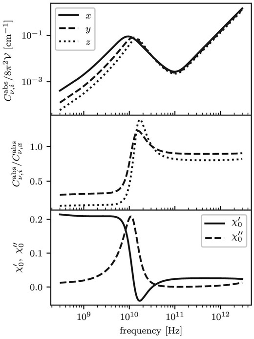
Frequency dependence of absorption cross-sections for an electric field parallel to each axis of an ellipsoid normalized by |$8 \pi ^2 \mathcal {V}$| (top panel), of relative absorption cross-sections for an electric field parallel to the semi-middle and semi-minor axis to that of the semi-major axis (middle panel), and of the real and imaginary parts of the electric susceptibility for spherical dust (bottom panel). A ratio of geometric factors is fixed to |$L_x : L_y : L_z = 1 : 2 : 3$|. Other parameters are set to the best-fitting values for W 43 listed in table 2.
The degree of polarization |$\Pi _\nu$| is obtained by taking the ratio of |$|\langle C_\nu ^\mathrm{pol} \rangle |$| to |$|\langle C_\nu ^\mathrm{abs} \rangle |$|. Figure 6 shows the frequency dependence of |$\Pi _\nu$| on the thermal emission from amorphous silicate dust. In the frequency range, except in the waveband around the resonance peak, |$\Pi _\nu$| is nearly constant. Since |$\langle C_\nu ^\mathrm{pol}\rangle$| takes a positive value, the direction of polarization is perpendicular to the magnetic field, as expected. Since the imaginary part of the susceptibility, |$\chi _0^{\prime \prime }$|, is much smaller than the real part, |$\chi _0^{\prime }$|, in these frequency ranges, the ensemble averages of the absorption and polarization cross-sections are expressed as |$\langle C_\nu ^\mathrm{abs} \rangle = \chi _0^{\prime \prime } f(\chi _0^{\prime })$| and |$\langle C_\nu ^\mathrm{pol} \rangle = \chi _0^{\prime \prime } g(\chi _0^{\prime })$| in the first-order of the imaginary part. Therefore, |$\Pi _\nu$| is independent of |$\chi _0^{\prime \prime }$| and depends only on |$\chi _0^{\prime }$|. Since the frequency dependence of |$\chi _0^{\prime }$| is very small, |$\Pi _\nu$| of the high and low frequency ranges, except around the resonance peak, become almost constant against frequency change. In the high frequency range, the DCD contribution of |$\chi _0^{\prime }$| is dominant. On the other hand, in the low frequency part, the contribution of the resonance process to |$\chi _0^{\prime }$| is dominant. This results in the discrepancy of |$\Pi _\nu$| found in figure 6 between the high and low frequency regions across the resonance peak.
Parameter dependences of the degree of polarization of the thermal emission from amorphous silicate dust as a function of frequency. For reference, the polarization degree with the same parameter set is shown by a solid line in each panel. The fraction of the atoms trapped in the TLS is set to be 0.01. In each panel, one of the variables characterizing the amorphous silicate dust is varied with respect to the reference model to see how the shape of the polarization degree responds to each variable. In the case of |$\Delta _0^\mathrm{max}/h = 100\:$|GHz shown in panel (a), |$\langle C_\nu ^\mathrm{pol}\rangle$| defined by equation (21) takes negative values between 100 and 500 GHz. The polarization cross-sections take positive values for all other cases shown in these figures. The variables are (a) |$\Delta _0^\mathrm{max}$|, expressed in the corresponding frequency normalized by |$h$|, (b) |$R_{\Delta }$|, (c) |$T$|, (d) |$\tau _+$|, and (e) |$L_\mathrm{min}$|, respectively. The given values for each parameter are shown in the legends.
At around the resonance peak, the degree of polarization shows a prominent behavior for some sets of parameters. Figures 6a and 6d show that the degree of polarization decreases abruptly and takes the local minima around the peak frequency of the resonance process when |$\Delta _0^\mathrm{max} > h/\tau _+$|. This is because the amplitude of the polarization cross-sections for all three axes of the ellipsoid get closer near the resonance peak, as shown in figure 5. As a result, the polarization cross-section defined by equation (21) approaches zero. In extreme cases, the polarization cross-section changes its sign. This can be seen in the case of |$\Delta _0^\mathrm{max}/h = 100\:$|GHz in figure 6a. In this case, the order of the amplitude of the absorption cross-section reverses: |$\langle C_{\nu ,x}^\mathrm{abs} \rangle < \langle C_{\nu ,y}^\mathrm{abs} \rangle < \langle C_{\nu ,z}^\mathrm{abs} \rangle$|. As a result, |$\langle C_\nu ^\mathrm{pol} \rangle$| becomes negative. This means that the direction of the polarization changes and becomes parallel to the magnetic field near the resonance peak frequency. Figure 6c shows that the polarization degree takes a minimum value at the resonance peak when the temperature of the dust is as low as 10 K. This is because the relative intensity of the resonance peak to far-infrared emission increases when the dust temperature decreases, as shown in figure 2c.
4.2 Comparison with astronomical data
There is no definite report on the detection of the polarization from AME. The upper limits on |$\Pi _\nu$| for the Perseus MC and W 43 are given by Génova-Santos et al. (2015) and Génova-Santos et al. (2017), respectively. In this subsection, we attempt to fit intensity and polarization data simultaneously with our model.
4.2.1 Polarization SED data and modeling
In figure 7, the polarized SEDs for the Perseus MC and W 43 are shown. The data for polarized AME are taken from table 4 in Génova-Santos et al. (2015) and table 8 in Génova-Santos et al. (2017). We exclude the DRAO 1.4-GHz data point because Génova-Santos et al. (2017) suspected that Faraday rotation affects the data point. The polarization fluxes at 143, 217, and 353 GHz are extracted from the Planck second data release (Planck Collaboration 2016) using the same method adopted in Génova-Santos et al. (2017). Although the data point at 23 GHz quoted from WMAP indicates the detection of polarization, we cannot reject the possibility that the subtraction of the Galactic synchrotron contribution might be insufficient, and that the contribution of the Galactic synchrotron is dominant in the data point (Génova-Santos et al. 2017). Therefore, we treat this point as the upper limit when the fit is performed. The central values of the data points where the upper limits are given are set to zero.
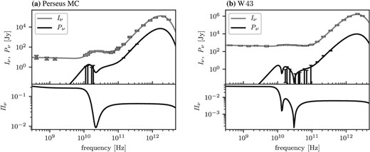
Intensity and polarized SEDs, and the polarization fraction for (a) the Perseus MC and (b) W 43. The error bars are |$1\sigma$| but the upper limits are at the 95% confidence level.
The intensity and polarization SEDs of ellipsoidal amorphous silicate dust are given by substituting equations (20) and (21) for equation (10). We include |$L_\mathrm{min}$| among the fit parameters. The free–free emission is assumed to be unpolarized.
4.2.2 Fit results
The observed SEDs of the intensity and polarization flux are fitted simultaneously. The brute-force fitting method adopted in sub-subsection 3.3.2 is used. The best-fitting parameters are summarized in table 3. The model predictions of the polarized SED with these best-fitting parameters are overlaid on the observed SED in figure 7.
It shows that our model is able to reproduce the overall features of both the intensity and polarization SEDs simultaneously. In the best-fitting model for the Perseus MC, there is a valley in the frequency dependence of the polarization fraction, and the polarization fraction reaches its minimum value at 20 GHz. The polarization fraction increases abruptly toward lower frequencies and approaches the asymptotic value. The asymptotic polarization fraction is factor of 5 larger than the polarization fraction in submillimeter wavebands. The model prediction is marginally consistent with the QUIJOTE 2|$\sigma$| upper limits but is slightly higher than the QUIJOTE upper limits in several frequency bands. In the best-fitting model for W 43, there is a dip in the polarization fraction defined by the ratio of equation (21) to equation (20) from 10 to 50 GHz. In this case, |$\langle C_\nu ^\mathrm{pol}\rangle$| changes sign from 13 to 30 GHz. Therefore, a 90-degree flip in the polarization direction in this frequency range is predicted. The polarization fraction below 10 GHz is factor of 10 larger than the polarization fraction in submillimeter wavebands. The model prediction is marginally consistent with the QUIJOTE |$2\sigma$| upper limits but is slightly higher than the QUIJOTE upper limits in several frequency bands.
5 Properties of the amorphous silicate dust
To reproduce the relative intensity of AME to the far-infrared peak intensity, our model requires very different physical characteristics for amorphous silicate dust in comparison with those of amorphous silicate materials found in the laboratory. In the laboratory, the fraction of atoms trapped in the TLS is reckoned to be of the order of |$10^{-4}$|. This comes from reproducing the experimental fact that the diagnostics dominated by the TLS in the heat capacity only appears below 1 K (Phillips 1987). On the other hand, for amorphous silicate dust, the required fraction of atoms trapped in the TLS is a few percent in order to reproduce the observed ratio of the AME peak intensity to the far-infrared peak intensity with a dust temperature of about 20 K. Figure 8 shows the frequency dependence of the absorption efficiency |$Q^\mathrm{abs}_\nu$|, which is the absorption cross-section normalized by the geometrical cross-section, of spherical amorphous silicate dust for various TLS fractions. It shows that the peak value of the absorption efficiency of the resonance process of the TLS with |$f_\mathrm{TLS} = 1$| is a factor of 5 larger than the absorption efficiency at 2 THz where the far-infrared peak appears. As shown in equation (10), the thermal emission spectrum is the product of the absorption cross-section and the Planck function |$B_\nu (T)$|. The ratio of the value of |$B_{20\:\rm GHz}(20\:\mbox{K})$| at the peak frequency of AME to |$B_{2{\mathrm{THz}}}(20\:\mbox{K})$| at the frequency of the far-infrared peak is about 0.0025. Therefore, |$f_\mathrm{TLS} \sim 10^{-2}$| is required to reproduce the observed ratio of the peak intensity of AME to the far-infrared peak intensity of |$10^{-4}$|. Figure 8 also shows that the peak value of the absorption cross-section of the resonance process of the TLS is two orders of magnitude less than the geometrical cross-section, even in the case where |$f_\mathrm{TLS} = 1$|. It shows that this is two orders of magnitude less than the absorption cross-section adopted by Jones (2009). Therefore, his predicted SED due to the resonance process of the TLS was two orders of magnitude overestimated.
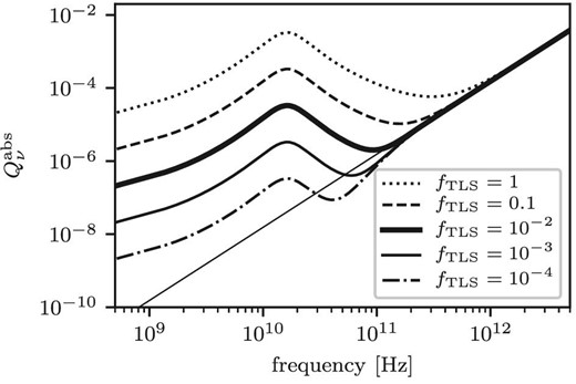
Frequency dependences of absorption efficiencies for spherical amorphous silicate dust. The given values of |$f_\mathrm{TLS}$| are shown in the legends. For the other parameters, the best-fitting parameter values for the Perseus MC listed in table 2 are adopted. The thin solid line is the absorption efficiency provided by the Draine and Lee (1984) model.
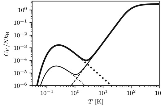
Temperature dependence of the heat capacities of the amorphous silicate dust in each MC predicted by our model. The contributions from the TLS are shown by a thick dotted curve for the Perseus MC and a thin dotted curve for W 43. The contribution from the Debye model shown by the dashed curve is the same for both MCs. The thick and thin solid curves are the total heat capacities for the Perseus MC and W 43, respectively.
Speck, Whittington, and Hofmeister (2011) proposed the possible forms of amorphous silicate dust in space. If a few percent of atoms are trapped in the double-well potential caused by deformation of the crystal structure, our results are applicable to any forms of amorphous silicate dust. The classic 10-|$\mu \mathrm{m}$| amorphous silicate feature observed in the interstellar medium (Knacke et al. 1969; Hackwell et al. 1970) is not affected by this.
6 Limitation of the present model and possible improvements
Although our amorphous models reproduce the observed intensity SEDs for the Perseus MC and W 43, the fits were not satisfactory. Our models underestimate the observed intensities in the frequency range from 100 GHz through 500 GHz. The model prediction of the polarization fraction of AME is slightly higher than the QUIJOTE upper limits in several frequency bands. The model prediction of the polarization fraction below 10 GHz is too high compared with that for submillimeter frequencies. Possible improvements to our model for each unsatisfactory point will now be discussed.
The TLS model describes the very low temperature limit of the soft-potential model. By fully taking into account the soft-potential model, the model SED above 100 GHz could be improved. The TLS describes the physical behavior of amorphous materials below 1 K. There are still deviations in the heat capacity from the Debye model in amorphous materials above 1 K, and the deviation at temperatures above 1 K is different from that below 1 K. The plateau in the heat conductivity at |$T {\sim} 1$|–|$100\:$|K is also found in amorphous materials (Zeller & Pohl 1971). These anomalous properties of amorphous materials cannot be explained by the standard TLS model alone. Karpov et al. (1982) proposed the soft-potential model as a model that surpasses the standard TLS model. The soft-potential model treats the double-well potential as the quartic function of the position of an atom. The standard TLS model is incorporated in the soft-potential model as its very low temperature limit. Since the typical temperature of interstellar dust is about 20 K, the physical processes beyond the standard TLS model may have a significant effect on the SED of the thermal emission from amorphous dust above 100 GHz.
One of the possibilities for reducing the model prediction of the polarization fraction in AME frequency bands is to replace the current DCD model by some other model that provides a higher value of the real part of the electric susceptibility |$\chi _0$| than that of the current DCD model. Figure 10 shows how the polarization fraction depends on the real part of the electric susceptibility (|$\chi _0^{\prime }$|). The plots calculated for various ratios of the imaginary part to the real part of the electric susceptibility (|$\chi _0^{\prime \prime }/\chi _0^{\prime }$|) are shown. The polarization fraction increases monotonically with increasing |$\chi _0^{\prime }$|. As the ratio of the imaginary part to the real part decreases, the polarization fraction converges to the asymptotic value for each value of |$\chi _0^{\prime }$|. This is because the polarization fraction depends only on the real part of the electric susceptibility when the imaginary part is much smaller than the real part, as shown in subsection 4.1. When the ratio is less than 0.1, the polarization fraction is proportional to |$\chi _0^{\prime }$| below |$\chi _0^{\prime }<0.2$|. Therefore, by replacing the current DCD model by some other model that provides a higher value of |$\chi _0^{\prime }$|, the ellipticity required to reproduce the observed polarization fraction in submillimeter wavebands is expected to be smaller than the current model; in other words, |$L_\mathrm{min}$| takes a value closer to |$1/3$|. As a result, a reduction is expected in our model predictions of the polarization fraction due to the resonance process of the TLS. Figure 11 compares the frequency dependence of the real and imaginary parts of the electric susceptibility predicted by our DCD model with that of Draine and Lee (1984) model. The imaginary parts of both models are identical in submillimeter wavebands. Therefore, the intensity SEDs in submillimeter wavebands would not be changed by replacing our DCD model with the Draine and Lee (1984) model. The real part is an order of magnitude larger than the imaginary part in submillimeter wavebands in both models. This shows that the real part of the Draine and Lee (1984) model is an order of magnitude larger than that of our DCD model. Therefore, replacing the current DCD model with the Draine and Lee (1984) one is one possible solution to reducing the model prediction of the polarization fraction with a small change in the model prediction of the intensity SED. A detailed quantitative study of this possibility is beyond the scope of the present paper and will be carried out in a forthcoming paper.
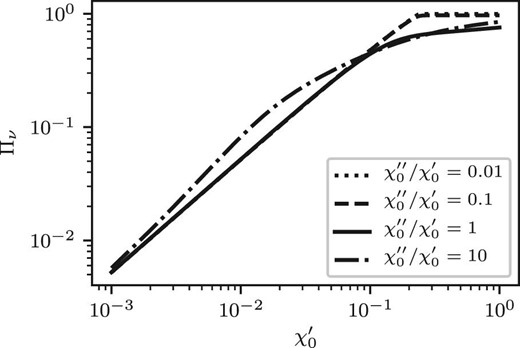
Polarization fraction as a function of the real part of the electric susceptibility (|$\chi _0^{\prime }$|) for various ratios of the imaginary part to the real part (|$\chi _0^{\prime \prime }/\chi _0^{\prime }$|). The dotted, dashed, solid, and dash–dotted curves correspond to |$\chi _0^{\prime \prime }/\chi _0^{\prime } = 0.01$|, 0.1, 1, and 10, respectively. The lower cut-off of |$L_x$|, |$L_\mathrm{min}$|, is set at 0.
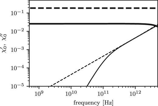
Comparison of frequency dependence of the electric susceptibility of our DCD model (solid curves) and the Draine and Lee (1984) model (dashed curves). Thick curves are real parts and thin curves are imaginary parts.
We have to mention that in the range of frequencies where AME is detected the interpretation of the nature of the polarization signals is quite complex. The total polarized emission could be increased or decreased because of a polarized synchrotron residual component. In addition to this, the band pass and the beam of the telescope could mitigate the total level of polarization of AME, particularly if this happens in the frequency range where the polarization of AME is expected to change sign.
Although we have neglected the contribution of the carbonaceous dust, it is known that amorphous carbon dust is closer to the realistic form of carbonaceous dust in the interstellar medium (Zubko et al. 1996) and almost half of the mass of interstellar dust is shared by carbonaceous dust (Hirashita & Yan 2009). Since the physical processes of the TLS are universal among the amorphous materials and independent from elemental compositions, intensity and polarization SEDs of thermal emission from amorphous dust derived in this paper are applicable to the amorphous carbon dust. However, the physical parameters which described the TLS of the amorphous carbon dust could be different from those of the amorphous silicate dust. In addition, free electrons might contribute to the electric susceptibility of the amorphous carbon dust. Further, amorphous carbon dust might have an isotropic structure (Draine & Lee 1984). This results in the anisotropic dielectric function tensor. Since the main scope of this paper is providing the framework to evaluate the intensity and polarization SEDs of thermal emission from amorphous dust by self-consistently taking into account the TLS model and demonstrating that this model is promising, the studies of the effect of the amorphous carbon dust on SEDs are beyond the scope of this paper and are shown in a forthcoming paper.
Although we assumed that all dust grains stayed at the same temperature, significant time variations of the temperature of the small dust grains are expected according to the stochasticity of the heating process (e.g., Draine & Li 2001). In a significant fraction of time, small dust grains stay at a much lower temperature than that of the large dust grain which is defined by thermal equilibrium. As shown in figure 2c, the relative intensity of the emission from the resonance process to the contribution from the lattice vibration becomes higher as the dust temperature becomes lower. Therefore, quantitative studies of the stochastic heating and size distribution of the dust grains are important.
As shown in figure 4, there are significant differences in the shapes of the spectra of the thermal emission from amorphous dust between the Perseus and W 43 MCs. The variation of the spectra shape originates from the fact that the physical parameters describing the amorphous dust, such as |$\Delta _0^\mathrm{max}$|, |$R_\Delta$|, |$\tau _+$|, and |$f_\mathrm{TLS}$|, take different values for each MC (see table 2). Possible origins of the variations are now summarized.
(1) The elemental composition of amorphous silicate dust is different for the Perseus MC and W 43. The shape of SEDs is sensitive to the values of |$\Delta _0^\mathrm{max}$| and |$R_\Delta$|. The peak frequency and width of the AME spectra due to the resonance process in the standard TLS model are defined by |$\Delta _0^\mathrm{max}$| and |$R_\Delta$|, respectively. As presented in equation (A7), |$\Delta _0$| is directly related to the tunneling parameter |$\lambda$|. The value of the tunneling parameter depends on the masses of the atoms constituting amorphous silicate dust, and the width and height of the potential barrier of the double-well potential in which an atom is trapped. It is natural that the typical values of these parameters change if the elementary composition of amorphous silicate dust is different. In this paper, we have assumed the number ratio of Fe to Mg in the amorphous silicate dust to be 1 to 1 (see table 1), however, that value might be different in each MC. Although we have not considered contributions from amorphous carbon dust in SEDs, there are several arguments that indicate their existence (e.g., Compiègne et al. 2011; Jones et al. 2017). It may also affect the spectral shape of AME. Since the elemental composition of the amorphous carbon dust is expected to be insensitive to the environmental metal abundance, the variations of the |$\Delta _0^\mathrm{max}$| and |$R_\Delta$| of the amorphous carbon dust among the MCs could not be attributed to the variation of the metal abundance of the environment.
(2) Differences of cooling processes which solidify gas and form an amorphous dust in each MC may result in a variation of the bonding structure of the atoms in the dust and in a variation in the amorphous nature of a dust particle. Amorphous materials are generated by rapid cooling from the liquid phase to the solid phase in the laboratory. In interstellar space, the solidification may happen from the gas phase without passing through the liquid phase in an extremely low pressure environment. This could be one of the sources for which |$f_\mathrm{TLS}$| takes an extremely high value compared with terrestrial amorphous materials.
(3) Since the shape of the AME spectrum depends sensitively on the shape of the spectrum of free–free emission in the microwave region, which depends sensitively on the temperature of the ionized gas, it is possible that component separation between the free–free emission and AME is not sufficient. If the magnitude or shape of the free–free emission SED changes, the best-fitting values of these parameters also change easily.
The fact of the lack of AME in cold dense cores (Tibbs et al. 2016) could be explained by a kind of variation in the amorphous nature of the dust due to a difference in environmental conditions.
7 Conclusions
Complete studies of the radiative processes of thermal emission from amorphous dust from the millimeter through far-infrared wavebands were presented by, for the first time, self-consistently taking into account the standard TLS model. How the intensity and the polarization SEDs respond in physical parameters characterizing the standard TLS model was shown. The amorphous model could reproduce the observed SEDs from AME up to the far-infrared feature very well. In our models, AME is originated mainly from the resonance emission of the TLS of large grains. The amorphous model is able to explain AME without introducing new species. Simultaneous fitting of the polarization and intensity SED for the Perseus MC and W 43 were also performed. Since there is no definite detection of polarization emission from AME, the adopted polarization intensities in the AME frequency range were upper limits. The polarization intensities measured by Planck at 143, 217, and 353 GHz were also included. The amorphous model could reproduce the overall observed feature of the intensity and polarization SEDs of the Perseus MC and W 43. However, the model prediction of the polarization fraction of AME was slightly higher than the QUIJOTE upper limits in several frequency bands. Possible improvements to our model to resolve this problem were proposed in the previous section. Our model predicts that amorphous silicate dust have very different physical characteristics compared with amorphous silicate materials found in the laboratory. We have shown that thermal emission from amorphous dust is an attractive alternative possibility as the origin of AME.
Acknowledgements
We thank Tetsuo Yamamoto for helpful discussions throughout the course of this work. We thank the referee, Itsuki Sakon, for constructive comments. We thank T.J. Mahoney for revising the English of the draft. MN acknowledges support from the Graduate Program on Physics for the Universe (GP-PU), Tohoku University. FP acknowledges the European Commission and the MINECO. This work is partially supported by MEXT KAKENHI Grant Number 18H05539 and MEXT KAKENHI Grant Number 18H01250. This project has been partially funded by the European Union’s Horizon 2020 research and innovation programme under grant agreement number 687312 (RADIOFOREGROUNDS), and by the SPACE IR MISSIONS II project under grants agreements ESP2015-65597-C4-4-R and ESP2017-86852-C4-2-R, respectively. MH would like to express his sincere condolences to Prof. Tsai An-Pang who was the world authority on quasicrystal and passed away in May 2019 at age of 60. In the course of this study, as the resident who lived in the same apartment by chance, MH received fruitful comments on the study and great support in the private life.
Appendix 1 Standard TLS model
There are two main relaxation processes. One is quantum tunneling, in which an atom passes through the potential barrier by the quantum effect. The other is hopping, where an atom climbs over the barrier by gaining enough energy due to thermal fluctuation.
Appendix 2 Extension of the Clausius–Mossotti relation for an ellipsoidal particle
Appendix 3 General optical properties of ellipsoidal particle
Footnotes
We define |$\chi $| and |$\chi _0 $| as susceptibilities for the response to a macroscopic internal electric field and to an external electric field, respectively. |$\chi $| is related to an electric permittivity |$\varepsilon $| as |$\varepsilon = 1 + 4 \pi \chi $|.
References
