


Abstract
We propose a new observing method for single-dish millimeter and submillimeter spectroscopy using a heterodyne receiver equipped with a frequency-modulating local oscillator (FMLO). Unlike conventional switching methods, which extract astronomical signals by subtracting the reference spectra of off-sources from those of on-sources, the FMLO method does not need to obtain any off-source spectra; rather, it estimates them from the on-source spectra themselves. The principle uses high-dump-rate (10 Hz) spectroscopy with radio frequency modulation achieved by fast sweeping of a local oscillator of a heterodyne receiver. Because sky emission (i.e., off-source) fluctuates as |$1/f$| and is spectrally correlated, it can be estimated and subtracted from time series spectra (a timestream) by principal component analysis. Meanwhile, astronomical signals remain in the timestream since they are modulated to a higher time-frequency domain. The FMLO method therefore achieves (1) a remarkably high observation efficiency, (2) reduced spectral baseline wiggles, and (3) software-based sideband separation. We developed an FMLO system for the Nobeyama |$45\:$|m telescope and a data reduction procedure for it. Frequency modulation was realized by a tunable and programmable first local oscillator. With observations of Galactic sources, we demonstrate that the observation efficiency of the FMLO method is dramatically improved compared to conventional switching methods. Specifically, we find that the time to achieve the same noise level is reduced by a factor of 3.0 in single-pointed observations and by a factor of 1.2 in mapping observations. The FMLO method can be applied to observations of fainter (|$\sim$|mK) spectral lines and larger (|$\sim$|deg|$^{2}$|) mapping. It offers much more efficient and baseline-stable observations compared to conventional switching methods.
1 Introduction
Improving the sensitivity of a single-dish radio telescope system is always an important issue in modern observational astronomy, especially in the era of the Atacama Large Millimeter/submillimeter Array (ALMA). Detecting faint molecular line emission by single-dish blind redshift spectroscopic surveys is essential to studying distant submillimeter galaxies (SMGs; e.g., Blain et al. 2002) with great help from the large collecting area (e.g., Yun et al. 2015). Efficient single-dish mapping spectroscopy is also important to ALMA itself as ALMA uses four single-dish antennas (Total Power Array of the Atacama Compact Array) in order to improve the fidelity of interferometric images.
The conventional position switching (PSW) and frequency switching (FSW) methods have been widely used in single-pointed1 spectroscopic observations in (sub-)millimeter astronomy (Wilson et al. 2012). These switching methods are necessary to estimate and correct for bandpass gains and sky levels based on a comparison of reference spectra, with the major assumption that the condition of the telescope (i.e., bandpass and receiver noise temperature) and atmosphere (i.e., opacity) can be regarded as being constant in the time interval between on- and off-points2 or frequency shift from one to another. In both methods, however, making a comparison (i.e., subtraction) with a reference spectrum is virtually equivalent to an addition of noise to the on-point spectrum, which is why the factor of |$\sqrt{2}$| is multiplied on the right-hand side of equation (1).
Another issue is the spectral baseline fluctuation across emission-free channels. The incident sky emission is generally time variable and inhomogeneous at (sub-)millimeter wavelengths (Lay & Halverson 2000). When the switching periods between on- and off-points (or frequency shift) are longer than the typical timescale of sky variations, imbalance between two spectra can cause baseline fluctuations in the resulting spectra, because the conventional chopper wheel method does not deal with in situ estimation of bandpass gains and sky levels.
The resulting |$\eta _{\rm obs}$| offered by the PSW method is therefore not so high (|$0.1 \lesssim \eta _{\rm obs} < 0.5$|) because of off-point measurements, telescope slewing time between on- and off-points, and some “flagging” of bad spectra due to baseline fluctuations. As an improvement of the PSW method, a novel method that uses a smoothed off-point bandpass (Yamaki et al. 2012) in order to reduce the noise added by the subtraction is a good compromise, offering |$0.5 < \eta _{\rm obs} < 1$|. As for observing an extended region, the on-the-fly (OTF) mapping method (Sawada et al. 2008) is more efficient because it continuously drives an antenna to cover the region rapidly, and measurements of the off-point are only taken between scans. These improvements, however, still require off-point measurements, and the degrading of |$\eta _{\rm obs}$| is still possible.
On the other hand, the |$\eta _{\rm obs}$| offered by the FSW method is higher (|$\eta _{\rm obs} > 0.5$|). The targets of the method, however, are limited to narrow spectral features such as Galactic quiescent sources because the line width must be narrower than the frequency shift. To improve the FSW method, Heiles (2007) has proposed obtaining spectra with more than two frequencies and then directly solving and correcting for IF-dependent bandpass gains by least-squares fitting (least-squares frequency switch; LSFS). This approach assumes that the RF spectral shape should remain constant throughout an observation, and thus any spectral undulation due to non-linear response to variable atmospheric emission and receiver gain will result in systematic errors.
In contrast, a method achieving a high observation efficiency (|$\eta _{\rm obs} \approx 0.9$|–1) that never needs off-point measurements has been developed; furthermore, it has been extensively employed in recent deep extragalactic surveys and cosmic microwave background (CMB) experiments on the basis of ground-based facilities using multi-pixel direct detector cameras. The output of a ground-based telescope is always dominated by the atmospheric emission. If a receiver has array detectors (e.g., a multibeam receiver or a spectrometer), the output time series data (timestream, hereafter) from the detectors are mutually correlated, because the detectors see almost the same part of the troposphere (|${\sim } 1$| km above the ground). Because these correlated noises are known to behave as |$1/f$|-type noises and have large power at low frequencies (|${\lesssim } 10$| Hz) in the timestream, filtering out the correlate modes of the timestream that are common among multiple detector outputs with, for example, principal component analysis (PCA) can provide in situ estimates and remove the awkward low-frequency noises induced mainly by the atmosphere (Laurent et al. 2005; Scott et al. 2008). At the same time, it is also important to modulate the astronomical signals involved in the timestream into higher-frequency domains so as not to filter out the astronomical signals of interest (Kovács 2008). In the continuum deep surveys and CMB experiments, this modulation is achieved by quickly moving the telescope pointing across the sky.
In this paper we report on the principle, instrumentation, and an observational demonstration of the FMLO method. We introduce the principle of the FMLO method in section 2 with the mathematical expression of a timestream. In Section 3 we describe the FMLO system of a telescope and its requirements, and the data reduction procedure after an FMLO observation. We then demonstrate single-pointed and mapping observations of the FMLO method for Galactic bright sources with the FMLO system on the Nobeyama |$45\:$|m telescope in section 4. We also verify how the resulting spectra obtained with the FMLO method are consistent with those obtained with the conventional method with a remarkable improvement of |$\eta _{\rm obs}$|. Finally, we discuss the advantages and limitations of the FMLO method in section 5.
2 Principle
We introduce the principle of frequency modulation and demodulation of a timestream, a series of frequency-modulated spectra, as illustrated in figures 1 and 2. We develop mathematical operations for frequency modulation and demodulation for both the signal and image sidebands. We then introduce a reduction for generating a cleaned timestream that corresponds to |$T_{\rm A}^{\ast }$| (antenna temperature corrected for atmospheric absorption and spillover loss) of the conventional PSW method. We reveal how the signal and noise are characterized in an intensity-calibrated timestream and how correlated components are defined and removed from it to make a cleaned timestream. Finally, we describe how we convert a cleaned timestream into a final spectrum (single-pointed observation) or a map cube (OTF mapping observation).
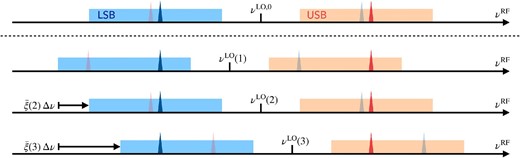
Schematic diagram showing modulation and demodulation of a timestream according to FM channels with mathematical expressions defined in subsections 2.1 and 2.2. It supposes an FMLO observation of both upper and lower sidebands (represented as colored boxes) where only one spectral line exists at each sideband (represented as colored spikes). Spikes with dimmed colors are the lines from the image sideband. A modulated timestream is the output of a spectrometer itself. On the other hand, a demodulated timestream is a matrix generated when we align each sample of the modulated timestream with the RF (sky) frequency (see also figure 2). It is clear that a line in a sideband and that contaminated from the image sideband are reverse frequency modulated, which enables us to achieve sideband separation in the post processing. (Color online)

Schematic diagram of reverse demodulation of a timestream. As we see in figure 1, demodulation according to FM channels with their signs reversed will align a timestream with the RF frequency of the image sideband. Such contamination can be modeled and subtracted if we integrate the reverse-demodulated timestream to generate a spectrum of contamination. (Color online)
2.1 Mathematical expression of timestreams
2.2 Modulation and demodulation of timestreams
2.3 Sideband separation with reverse demodulation
2.4 Observation equation
2.5 Correlated component removal
2.6 Making a final product
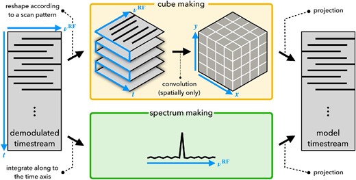
Schematic diagram of spectrum and map making. (Left) Demodulated timestream whose non-NaN values are expressed as black line segments. (Top center) Reshaped (folded) three-dimensional (3D) cube-like timestream according to a scan pattern of a mapping observation. Then the spatial convolution process converts the timestream into a 3D map cube. (Bottom center) Spectrum derived from the timestream integrated along the time axis. (Right) Demodulated model timestream of signal. In the case of a spectrum, a projection process generates a demodulated timestream in which each time sample is filled with a spectrum; the demodulated timestream is used to generate a modulated timestream. In the case of a map, a projection process converts a 3D map cube into a timestream whose shape is the same as that of the input timestream, which can be derived by 2D (spatial axes) interpolation of a 3D map cube at map coordinates at each observed time. (Color online)
2.7 Making a model timestream from a final product
As illustrated in figure 3, the model product is transformed into a demodulated model timestream, |$\widetilde{\boldsymbol {T}}^{\rm model}$|. In the case of a spectrum, it is a |$\widetilde{D} \times N$| matrix whose columns are filled with |$\widetilde{\boldsymbol {s}}^{\rm \, \, model}$|. In the case of a map, it is a |$\widetilde{D} \times N$| matrix whose |$n$|th column is a spectrum as a result of two-dimensional interpolation (i.e., |$x$| and |$y$| axes) of |$\widetilde{{\boldsymbol M}}^{\rm model}$| at its antenna coordinates.
3 Instrumentation
3.1 Hardware implementation
In the proposed FMLO method it is essential to modulate astronomical signals of interest into high time frequency ranges in a timestream by modulating the observing frequency, which allows for the isolation of astronomical signals from correlated noise of a low time frequency. Although there are several methods to modulate the frequency, we choose to modulate RF signals. This is because (1) in many modern systems, a first LO is realized with a computer-controlled signal generator in which a built-in modulation function is implemented, and (2) RF modulation in mm/submm allows for a wide (GHz-order) frequency change compared with IF modulation.
The minimum requisites for the telescope system on which the FMLO system is to be installed are as follows: (1) a tunable and programmable first LO; (2) a system clock that ensures synchronization between frequency modulation and data acquisition; and (3) a backend spectrometer that takes the data at a dump rate sufficiently higher than variations in the sky and system. A heterodyne receiver in modern mm/submm astronomy often utilizes a microwave signal generator with a cascade of frequency multipliers, instead of a Gunn oscillator, as a first LO. A digital signal generator is particularly useful for the purpose of the FMLO method, as it is easy to quickly tune the LO frequency and program the FM pattern. A dump rate of |$\sim$|10 Hz should be sufficient for many cases; the timescale of sky variation is of the order of |$\sim$|1 s, as it is roughly determined by the crossing time in which the phase screen (|$v \sim 10$| m s|$^{-1}$|) goes across the telescope aperture (|$D \sim 10$| m). Note that when we apply the FMLO method to OTF mapping rather than single-pointed observations, synchronization between frequency modulation and antenna drive control is also required.
As an example of hardware implementation we show a block diagram of an FMLO observing system on the Nobeyama |$45\:$|m (developed in 2013) in figure 4. The receiver system comprises the two-beam TZ front-end receiver with a cryogenic superconductor–insulator–superconductor (SIS) mixer (Nakajima et al. 2013) and the digital backend spectrometer SAM45, which is an exact copy of the ALMA ACA correlator (Kamazaki et al. 2012). In this study we just use a single IF (a single beam and a single polarization). We employ a signal generator, Agilent E8257D, which is capable of generating a continuous wave (CW) according to a frequency list given by an observer. Each frequency in the list is switched to by external TTL-compatible reference triggers in a sequential manner. The trigger is produced with an arbitrary waveform generator, Agilent E33521A. The waveform generator produces a rectangular wave with a period of 100 ms, which is synchronized with the telescope’s system clock via 1 pps and 10 MHz reference signals. The period must be identical to the dump rate of the spectrometer outputs (10 Hz), and the phase of the rectangular wave must be synchronized with the onset of data acquisition. This is made in the OTF mode of the Nobeyama |$45\:$|m (Sawada et al. 2008), while the telescope may focus on a single point in the sky. Figure 5 shows the voltages of the reference trigger and 1 pps signal as a function of time, which shows accurate enough synchronization. The typical error in synchronization is better than |${\sim } 200\, \mu$|s, which is well below the typical dwell time of a single frequency (100 ms). Note that it typically takes |${\lesssim } 8$| ms to settle the generated LO frequency after the frequency is set to one value from another. The Agilent E8257D does not output any CW signals during the interval in which the frequency settles to a programmed value, which makes the SIS device deactivate itself temporally, and thus the SIS is unavailable during the settling time. This causes a slight sensitivity loss of |${\lesssim } 4\%$| for a dwell time of 100 ms (i.e., |${}[(100-8)/100]^{1/2} \simeq 0.96$|). The decrease in astronomical signals is corrected for in an absolute intensity calibration.
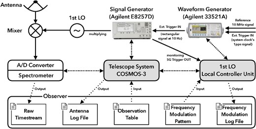
Block diagram of an FMLO system on the Nobeyama |$45\:$|m. The solid and dashed arrows indicate the directions of signals and data communications between instruments and an observer, respectively. The diagram has three layers. (Top) The frontend receiver system, where the RF signal from the sky and frequency-modulated LO signal are mixed at the SIS device and a subsequent IF signal is input to the spectrometer after analog-to-digital conversion. (Middle) The backend spectrometer and the telescope system, COSMOS-3. (Bottom) An observer who sends and receives inputs and outputs. (Color online)
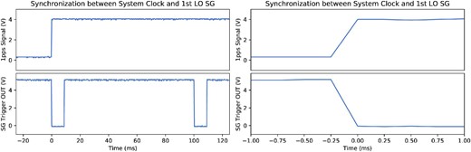
Measured signals of the 1 pps system clock (top) and first LO signal generator’s reference trigger (bottom) of the Nobeyama |$45\:$|m telescope in volts. The left panels show them over a |$\Delta t = 150$| ms duration, where the 1 pps signal rises at |$t=0$| ms, while the trigger signal, which is synchronized with the 1 pps clock, falls. The subsequent |$\Delta t \simeq 8$| ms voltage dropping at 0 V is attributed to the settling time of the signal generator, where it does not generate a signal for the LO; thus, the SIS mixer is unavailable. The right panels show the same results, but over a |$\Delta t = 2$| ms duration around |$t=0$| ms, which demonstrates that the time synchronization error is much better than |$200\, \mu$|s, the period of a slope. (Color online)
A typical procedure for an FMLO observation of the Nobeyama |$45\:$|m is as follows. The data and signal flow are shown at the bottom of figure 4.
The Nobeyama |$45\:$|m telescope system (COSMOS-3; Morita et al. 2003; Kamazaki et al. 2005) loads a script for an FMLO observation (observation table); then the local controller unit (LCU) reads a frequency list (FM pattern file) and sends it to the signal generator.
Once the telescope begins stable tracking, the receiver is properly tuned, and at this time the spectrometer is ready to record; then, the LCU triggers the signal generator when data acquisition starts.
During an observation, the spectrometer records time series spectra of an on-point at a dump rate of 10 Hz while it regularly takes measurements of a hot load (chopper wheel) at the reference frequency for an absolute intensity calibration (typically once every 30 min). At the same time, the LCU logs incident information about the frequency, timestamp, and Doppler tracking of the receiver into a frequency modulation log file.
After the observation, an observer obtains a raw timestream, an antenna log file that contains time series antenna coordinates, and a frequency modulation log file that contains actual time series FM values generated by an LO.
3.2 Data reduction procedure
After an FMLO observation, the succeeding data reduction is conducted offline to make a final product (a spectrum or map). It is thus necessary to handle outputs properly and apply the signal processing methods to them according to the equations described in section 2. We merge such outputs into a single file, the format of which is independent of hardware implementation, and create and operate a two-dimensional array representing a modulated timestream of on-point spectra, which is loaded from the file in an offline pipeline program. We choose to use FITS (flexible image transport system) as the file format and have developed a Python-based data analysis package, FMFlow.6 It provides functions for timestream operations such as modulation and demodulation, correlated noise removal by PCA, and generating a final product from a timestream and vice versa (i.e., generating a model timestream from a final product).
In the data reduction process, it is also essential to implement an iterative algorithm to estimate |$\boldsymbol {T}^{\rm cor}$|, |$\boldsymbol {T}^{\rm ast(,i)}$|, and |$\boldsymbol {T}^{\rm atm(,i)}$| by turns. The iterative method was originally introduced by an iterative map-making algorithm for the bolometer array camera, SCUBA-2 (Chapin et al. 2013), in which map-based correlated components (referred to as common-mode) and astronomical signals were estimated. On the other hand, our method estimates them based on a spectrum and optimizes them for sideband separation, as mentioned in section 2. We show a flowchart of the iterative algorithm in figure 6. With a single estimate of the spectrum-based correlated components, an estimate of correlated noise, |$\hat{\boldsymbol {T}}^{\rm cor}$|, might be strongly affected by the line emission from the sky and/or astronomical signals.7 This usually yields negative sidelobe-like features around the line emission in the final spectrum. Such features can also be seen in the residual timestream, |$\hat{{\boldsymbol E}}^{\rm nc}$|, in the top right panel of figure 6. It is therefore necessary to model8|$\boldsymbol {T}^{\rm ast(,i)}$| and |$\boldsymbol {T}^{\rm atm(,i)}$|, and re-estimate |$\boldsymbol {T}^{\rm cor}$| from a timestream where |$\hat{\boldsymbol {T}}^{\rm ast(,i)}$| and |$\hat{\boldsymbol {T}}^{\rm atm(,i)}$| are subtracted. Such subsequent iterative processes can minimize any errors between an estimate and a “true” value as the estimate is converged after several iterations.
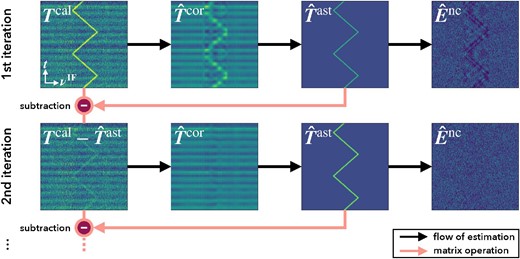
Flowchart of the iterative algorithm in an FMLO data reduction. For simplification, we show the case of no astronomical line emission from the image sideband (i.e., |$\boldsymbol {T}^{\rm cal}=\boldsymbol {T}^{\rm cor}+\boldsymbol {T}^{\rm ast}+{\boldsymbol E}^{\rm nc}$| is assumed). Each panel represents a simulated modulated timestream observed with a zigzag FM pattern (see also figure 7). We assume that there exists a strong line emission observed around the center of the spectrometer band. The top left panel shows the timestream of the measured antenna temperature, |$\boldsymbol {T}^{\rm cal}$|. The other panels in the top row show the estimates of the correlated components (|$\hat{\boldsymbol {T}}^{\rm cor}$|), astronomical line emission (|$\hat{\boldsymbol {T}}^{\rm ast}$|), and residual (|$\hat{{\boldsymbol E}}^{\rm nc}$|) in the first iteration. The bottom panels show the estimates of the correlate components in the second iteration. The estimation starts from |$\boldsymbol {T}^{\rm cal}$| with the subtraction of |$\hat{\boldsymbol {T}}^{\rm ast}$|, which results in better estimation of |$\hat{\boldsymbol {T}}^{\rm cor}$|. (Color online)
Set initial estimates of |$\boldsymbol {T}^{\rm ast(,i)}$| to zero (|$\hat{\boldsymbol {T}}^{\rm ast}=\hat{\boldsymbol {T}}^{\rm ast,i}={\bf 0}$|).
Estimate correlated components, |$\hat{\boldsymbol {T}}^{\rm cor}$|, by applying PCA to the timestream of |$\boldsymbol {T}^{\rm cal}-\hat{\boldsymbol {T}}^{\rm ast}-\hat{\boldsymbol {T}}^{\rm ast,i}$| [i.e.,, deriving |$\boldsymbol {X}^{\rm c}$| in equation (26), where |$\boldsymbol {X}=\boldsymbol {T}^{\rm cal}-\hat{\boldsymbol {T}}^{\rm ast}-\hat{\boldsymbol {T}}^{\rm ast,i}$|].
Estimate the astronomical line emission from the signal sideband, |$\hat{\boldsymbol {T}}^{\rm ast}$|, by modeling a timestream from the final product derived from |$\boldsymbol {T}^{\rm cal}-\hat{\boldsymbol {T}}^{\rm cor}-\hat{\boldsymbol {T}}^{\rm ast,i}$|.
Estimate the astronomical line emission from the image sideband, |$\hat{\boldsymbol {T}}^{\rm ast,i}$|, by modeling a timestream from the final product derived from |$\boldsymbol {T}^{\rm cal}-\hat{\boldsymbol {T}}^{\rm cor}-\hat{\boldsymbol {T}}^{\rm ast}$|.
Generate the cleaned timestream, |$\hat{\boldsymbol {T}}^{\rm cln} = \boldsymbol {T}^{\rm cal}-\hat{\boldsymbol {T}}^{\rm cor}-\hat{\boldsymbol {T}}^{\rm ast,i}$|. If |$\hat{\boldsymbol {T}}^{\rm cln}$| is converged (i.e., values are not significantly changed from the previous ones), the iterative algorithm is finished. Otherwise, return to step 2 and repeat until convergence is achieved.
4 Demonstration
We show the results of single-pointed and mapping observations with both the FMLO and PSW methods and demonstrate an improvement in observation efficiency for FMLO and consistency of intensity between the two methods. We use Galactic sources that have bright (|$T_{\rm A}^{\ast }\sim 10^{0-1}$| K at peak) emission lines at millimeter wavelengths and thus are usually observed as “standard sources” for absolute intensity calibration in a spectral line observation.
4.1 Observation efficiency and sensitivity improvement
4.2 Observations
We carried out the observations during the commissioning of the FMLO system on the Nobeyama |$45\:$|m telescope in early 2016 June and 2017 using the TZ front-end receiver and SAM45 backend spectrometer. With both FMLO and PSW observations, we configured the A7 array of SAM45 in the lower sideband (LSB; |$\nu ^{\rm RF}=97.98097$| GHz). We set the spectral channel spacing of SAM45 to 0.48828 MHz and the total bandwidth as 2000 MHz (4096 channels in total), which respectively correspond to 1.50 km s|$^{-1}$| and 6118 km s|$^{-1}$| in velocity at the observed frequency of 98 GHz.
With the FMLO observations, we recorded the output timestream data of the on-point at a rate of 10 Hz by the SAM45 spectrometer. At that time we used a zigzag-shaped function as the FM pattern, which has two free parameters, an FM width and an FM step, as illustrated in figure 7. By definition, the total observed bandwidth is the sum of the total bandwidth of the spectrometer and the FM width. This means that a wider FM width results in a wider total observed bandwidth but fewer samples at the edge of the demodulated timestreams. Thus, the sensitivity loss at the edge is greater than at the center of the observed band. On the other hand, a narrower FM width or shorter FM step may fail to estimate correlated and non-correlated components by PCA, when the frequency width of a target spectral line is wider than them, which might produce incorrect estimates of the spectral line. We therefore choose these two parameters such that the FM width is wider than the FWHM of a spectral line and the FM step is as wide as possible within the FM width in order to optimize the conditions above.
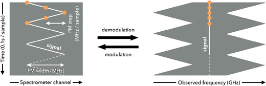
Schematic diagram of a zigzag FM pattern. (Left) Modulated timestream where the orange dots represent modulated signals fixed at the RF frequency. The FM width is the total modulation width over a timestream, and the FM step is an interval between successive time samples. (Right) Demodulated timestream where signals are aligned to the RF frequency. (Color online)
4.3 Data reduction
In the offline data reduction after an observation, we conducted two-channel binning of the timestream data to reduce the total number of channels by half to 2048 to reduce the computation time. We calibrated the absolute intensity of the data by the one-load chopper wheel method to derive atmospheric opacity-corrected antenna temperatures. In the case of the PSW data, we subtracted a linear baseline from each spectrum to make a final product.
In the case of the FMLO data we found that the power of the on-point timestream changes as the frequency is modulated, which indicates that the gain between power and temperature is not constant during an observation period between chopper measurements (typically, |$\sim$|15–30 min). We corrected for this FM-dependent gain by using the timestream data itself before the absolute intensity calibration: we applied the Savitzky–Golay smoothing filter (Savitzky & Golay 1964; window length of 51; polynomial order of 3) to a timestream of an on-point assuming that the gain change is only a function of the frequency modulation. Figure 8 demonstrates that the FM-dependent gain curve of an observation is fitted in the |$\nu ^{\rm LO}$|–power space and is corrected in the calibrated timestream, |$\boldsymbol {T}^{\rm cal}$|.
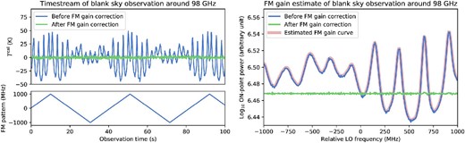
Demonstration of FM-dependent gain correction in a timestream in LSB around 98 GHz. The left panels show the antenna temperature of a modulated timestream, |$\boldsymbol {T}^{\rm cal}$|, at a channel of the band center and the corresponding FM pattern with observed time. The function of the FM pattern in the antenna temperature without FM-dependent gain correction (blue line) shows a clear trend. The right panel shows the power of the on-point at the same channel in the relative LO frequency versus log power space, where relative LO frequency is expressed as |$\nu ^{\rm LO}(n)-\nu ^{\rm LO,0}$|. The resulting FM-dependent gain curve by a Savitzky–Golay smoothing filter (pink line) is overlaid on the raw power (blue line). Both panels show the antenna temperature and power after correcting the FM-dependent gain (green lines). (Color online)
We then conducted the data reduction procedure of the FMLO method as described in subsection 3.2. We chose the number of principal components to model correlated components, |$K$|, such that the line-free channels of each timestream spectrum were flat enough to estimate the noise-free product (typically, |$K \simeq 5$| is used to conduct a |$\sigma$|-cutoff at |$\theta _{\rm cutoff}=5$|). We also chose the threshold value of convergence as |$\varepsilon = 0.05$|. In the case of a mapping observation, the atmospheric condition may have changed as the elevation of an antenna was not constant during an observation, which suggests that the eigenvectors of correlated components, |$\boldsymbol {P}$|, should be frequently estimated in a short period (several minutes). We split a timestream into many time chunks so that the time length of each chunk should be short enough (|$N\sim 600$|; |$\sim$|10 min) and applied correlated component removal to them independently.
We note that there could exist pointing errors between the PSW and FMLO observations of the same target induced by wind loads, temperature variation, and time-dependent deformation of the telescope dish. These errors cannot be corrected because we cannot observe them simultaneously with both methods, which may result in an intensity fluctuation in the spectral line emission between two observations (typically |$\pm$|10% in our commissioning). In the following subsections we therefore discuss the consistency of an FMLO observation with that of a PSW observation taking intensity fluctuation into consideration.
4.4 Blank-sky observation
Before turning our attention to the astronomical sources, we observed a blank sky (i.e., an off-point) with the FMLO method where no astronomical spectral lines are expected to exist. Such an observation can minimize the effect of astronomical signals and thus is suitable for the demonstration of, in particular, measuring noise levels and observation efficiency. We used an FM pattern whose FM width was 2000 MHz and FM step was 10 MHz per sample.
We verify how correlated component removal reduces low-frequency noise (|${\lesssim } 10$| Hz) in a cleaned timestream, |$\boldsymbol {T}^{\rm cln}$|, by measuring the power spectral densities (PSDs) and covariance matrices of a timestream before and after PCA cleaning. Figure 9 shows the results. As can be seen in the covariance matrix before PCA cleaning, correlated components remain in the timestream, |$\boldsymbol {T}^{\rm cal}$|. After correlated component removal, low-frequency noise at |$\lesssim$|0.1 Hz decreases by 1–2 orders of magnitude. A covariance matrix after PCA also shows no correlated components remaining compared to diagonal (auto-correlation) values.
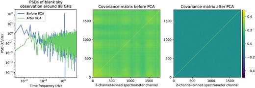
(Left) Power spectrum densities of the 98 GHz channel before and after PCA cleaning. Note that a strong line-like feature seen at |$\sim$|1.2 Hz is attributed to a periodic baseline bobbing caused by variation of a mechanical chiller for a heterodyne receiver. (Center) Covariance matrix created by |$\boldsymbol {T}^{\rm cal}$| (before PCA cleaning). (Right) Covariance matrix created by |$\boldsymbol {T}^{\rm cln}$| (after PCA cleaning). Note that the timestreams are normalized so that the diagonal values of the derived covariance matrix are unity. (Color online)
Figure 10 shows the final spectrum of a demodulated timestream, the 1 |$\sigma$| noise level evaluated from the timestream itself calculated by using equation (42)—with |$\alpha _{\rm FMLO}=1$|—and the 1 |$\sigma$| noise level which is expected to be achieved with a PSW observation of the same observation time. The noise level curve of a timestream is estimated by the bootstrap method by randomly changing the signs of samples of demodulated residual timestreams to resample the final spectra and derive the standard deviation. As the number of samples (|$\propto$| on-source time) of each frequency channel of the demodulated timestreams depends on the FM pattern, the noise level gets worse near the edge of the spectrum. As a result, the factor of noise contribution from correlated component removal is achieved as |$\alpha _{\rm FMLO}\sim 1.1$| over the observed band. In other words, equivalent noise from the off-point is |$\Delta T_{\rm off}=\sqrt{1.1^{2}-1^{2}}\, (T_{\rm sys}/\sqrt{\Delta \nu \, t_{\rm on}}) \sim 0.46T_{\rm sys}/\sqrt{\Delta \nu \, t_{\rm on}}$|, which means that accurate estimates of the in situ baseline achieved with the FMLO method more than double. We will discuss the actual value of |$\alpha _{\rm FMLO}$| in section 5.
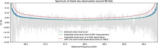
Final spectrum of a blank sky around 98 GHz (LSB) with atmospheric line emission subtracted (light blue line). We also plot (a) 1 |$\sigma$| noise level (standard deviation) derived from the timestream itself (green line), (b) 1 |$\sigma$| noise level expected to be achieved in R-SKY measurements (i.e., calculated from equation (42) with |$\alpha =1$|; red line), and (c) 1 |$\sigma$| noise level expected to be achieved with a PSW observation of the same total observation time as the FMLO observation (purple line). We derive the factor of noise contribution from correlated component removal, |$\alpha _{\rm FMLO}\sim 1.1$|, over the observed band estimated by dividing (a) by (b). Note that the two spectral dents seen at 96.3 GHz and 99.25 GHz are caused by atmospheric ozone lines, the subtraction of which is discussed in subsection 5.2. (Color online)
The achieved improvement in sensitivity of the FMLO method according to equation (43) is |$\iota =1.74$|; in other words, the FMLO observation requires only |$1/\iota ^{2}=33$|% of total observation time compared to PSW to achieve the same sensitivity of the final spectrum. In other words, we can equivalently observe with a telescope whose system noise temperature is |$(1-1/1.74)\sim 43$|% lower than the previous one.
In the actual observations, the observation efficiencies of both FMLO and PSW methods are lower than the ideal ones. For example, in the blank-sky observations we used for the verification, |$\eta _{\rm obs}^{\rm FMLO}$| and |$\eta _{\rm obs}^{\rm PSW}$| were 0.69 and 0.42, respectively. This is because, compared with typical scientific observations (on-source time of several hours), both observations were short (on-source time of 5 min) and the fraction of the overhead, such as the initial and final procedures of an observation, was large. Using the values of actual observing efficiencies, however, we achieved an improvement of |$\iota =1.65$|, which is almost the same value as the ideal one. We also note that the derived improvement, |$\iota$|, from this commissioning is the lower limit. When we conduct a scientific observation, |$\eta _{\rm obs}^{\rm PSW}$| is going to be much smaller because of the larger fraction of telescope slew time between the on- and off-points since the single observation time of each point should be short (|${<} 10$| s, for example) for better subtraction between two points.
4.5 Single-pointed observation
We observed CS |$J$| = 2–1 [hereafter CS (2–1); |$\nu _{\rm rest}=97.980953$| GHz; in LSB] of a carbon-rich star, IRC |$+$|10216, with an FM pattern whose FM width was 250 MHz and FM step 80 MHz per sample. The FM pattern fulfills the conditions above because the line width (full width at zero intensity; FWZI) of IRC |$+$|10216 is expected to be |${\sim } 40$| km s|$^{-1}$| (13 MHz) from past PSW observations (e.g., Cernicharo et al. 2010). The on-source time was |$40\times \eta _{\rm obs}^{\rm FMLO}$| s (400 samples) and the achieved noise level of the FMLO observation per spectral channel, |$\Delta T_{\rm FMLO}$|, was 0.046 K. Our references were PSW observations carried out four times at about an hour before and after the FMLO observation with the same observation conditions as the FMLO observation. Within each observation, we obtained 10 s of on- and off-point observations four times to achieve an on-source time of 40 s. The coordinates of the off-point were taken at |$6^{\prime }$| west of the on-point. The achieved noise level of the PSW observation adjacent to the FMLO observation was |$\Delta T_{\rm PSW}=0.057$| K.
Figure 11 shows the resulting FMLO spectrum of CS(2–1). We also show the PSW spectra, which were observed adjacent to the FMLO observation. These results show that the intensity can be easily changed within an hour beyond the noise level when we see a point-like source. Based on comparisons of the FMLO and PSW spectra taken at different times, however, we can still confirm that both the intensity and line shape of the FMLO spectra are consistent with those of PSW, as the intensity of the FMLO spectrum is between the minimum and the maximum of those of the PSW. To demonstrate the FMLO method for deeper spectral observation (mK order of noise level) in a future commissioning, it would be necessary to confirm the consistency of the FMLO method with the “time series” PSW measurements.
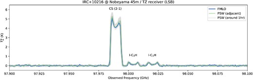
Obtained CS (2–1) spectra of IRC |$+$|10216 seen at 97.989 GHz observed with PSW (green line) and FMLO (blue one) methods at Nobeyama |$45\:$|m. We also plot various PSW spectra obtained around 60 min before and after the FMLO observation (gray lines) for monitoring typical pointing errors. Note that other two line features seen at 98.004 and 98.020 GHz are l-C|$_{3}$|H (Mauersberger et al. 1989; Agúndez et al. 2012). (Color online)
4.6 Mapping observation
4.6.1 Comparison
We made a raster-scan mapping observation of CS (2–1) toward the Orion KL |$10^{\prime \prime } \times 10^{\prime \prime }$| region using the Nobeyama |$45\:$|m telescope. We chose an FM pattern with FM width 120 MHz and FM step 40 MHz per sample. The FM pattern fulfills the conditions of the optimal FM pattern because the FWZI of Orion KL is expected to be |${\sim } 40$| km s|$^{-1}$| (15 MHz) from past PSW observations (e.g., the |$^{12}$|CO data cube of Shimajiri et al. 2011). Both conventional OTF and FMLO mapping observations were carried out with two raster-scan patterns: x-scan (each scan is made along right ascension axis) and y-scan (declination axis). The detailed parameters of the patterns are summarized in table 1. The typical system noise temperatures, |$T_{\rm sys}$|, during these observations were 230 K (LSB). As will be further described, the on-source time per spatial grid was 2.66 s (a factor of 92% is included) and the achieved noise level of the FMLO observation per spectral channel was 0.18 K (LSB) after applying map-making and basket-weaving methods (Emerson & Graeve 1988). Before and after the two FMLO mapping observations, conventional OTF mapping observations were carried out (the x-scan mapping was before them and the y-scan mapping was after). The typical |$T_{\rm sys}$| during these observations was 210 K (LSB). The on-source time per spatial grid was 2.90 s, and the achieved noise level of the FMLO observation per spectral channel was 0.15 K (LSB) after applying map-making and basket-weaving methods. The coordinates of the off-point was |$30^{\prime }$| east of the center of the mapping region.
Observational and data reduction parameters of OTF and FMLO observations.|$*$|
| OTF | FMLO | OTF | FMLO | |
|---|---|---|---|---|
| (|$10 \times 10$| arcmin|$^{2}$|) | (|$10 \times 10$| arcmin|$^{2}$|) | (|$1 \times 1$| deg|$^{2}$|) | (|$1 \times 1$| deg|$^{2}$|) | |
| |$l_{1}$| (|$^{\prime \prime }$|) | 600 | 600 | 1200 | 3600 |
| |$l_{2}$| (|$^{\prime \prime }$|) | 600 | 600 | 1200 | 3600 |
| |$\Delta l$| (|$^{\prime \prime }$|) | 6 | 6 | 6 | 6 |
| |$t_{\rm scan}$| (s) | 12 | 12 | 24 | 72 |
| |$t_{\rm off}$| (s) | 12 | 0 | 24 | 0 |
| |$t_{\rm tran}$| (s) | 5 | 5 | 5 | 5 |
| |$t^{\rm off}_{\rm tran}$| (s) | 10 | 0 | 10 | 0 |
| |$t_{\rm app}$| (s) | 5 | 5 | 5 | 5 |
| |$N_{\rm scan}^{\rm seq}$| | 3 | 101 | 1 | 601 |
| |$f_{\rm cal}$| | |$\simeq 1$| | |$\simeq 1$| | |$\simeq 1$| | |$\simeq 1$| |
| |$d$| (|$^{\prime \prime }$|) | 10 | 10 | 10 | 10 |
| |$\eta$| | 4.3 | 4.3 | 4.3 | 4.3 |
| |$t_{\rm OH}$| (s) | 15.0 | 10.0 | 25.0 | 10.0 |
| |$t^{\rm on}_{\rm cell}$| (s) | 1.45 | 1.33 | 1.44 | 1.32 |
| |$t^{\rm off}_{\rm cell}$| (s) | 20.0 | 0 | 40.0 | 0 |
| |$t^{\rm on}_{\rm total}$| (min) | 20.2 | 18.6 | 724 | 664 |
| |$t^{\rm obs}_{\rm total}$| (min) | 52.2 (58) | 37.0 (39) | 2201 | 821 |
| |$\eta _{\rm obs}^{\rm map}$| | 0.39 (0.35) | 0.50 (0.48) | 0.33 | 0.81 |
*The left two columns show the actual values used mapping observations toward the |$10 \times 10$| arcmin|$^{2}$| Orion KL region. The right two columns show the supposed values if we conduct |$1 \times 1$| deg|$^{2}$| mapping observations using OTF and the FMLO method, respectively. The three groups of rows represent: (Top) The observational parameters. If the values are different between OTF and FMLO, the better value is displayed in bold. (Middle) The parameters of map-making after obtaining mapping timestream data. |$\eta$| (not an observation efficiency) is a factor determined by the extent of the used GCF (|$\eta =4.3$| for a Bessel–Gauss GCF with default parameters). (Bottom) The derived values used for calculating observation efficiency. The values without parentheses are estimated values and those with parentheses are the actual values from timestream data and the observing logs.
After applying the basket-weaving method, we obtained a final FMLO map (3D cube) that is expected to be consistent with that of the OTF method (and also |$T_{\rm A}^{\ast }$|). Figure 12 shows the spectra obtained with the OTF and FMLO methods by averaging the spectra inside a |$30^{\prime \prime }$| radius of Orion KL. A comparison of the spectra obtained by the OTF and FMLO methods reveals that the FMLO spectrum obtained is almost consistent with that of the OTF. Figure 14 shows the integrated intensity maps of CS (2–1) created from the x-scan, y-scan, and basket-weaved 3D cubes. Comparisons between the OTF and FMLO maps of each row of figure 14 reveal that the overall spatial distribution and intensity of the FMLO maps are almost consistent with those of the OTF maps. Moreover, we demonstrate that the scanning effect (one of “correlated” components) seems to be removed in each raster scan of a single direction, while the large scanning effect remains in the the x- and y-scan of OTF maps along with their scan patterns before the basket-weaving method is used. After basket-weaving, both strong and weak structures seem to be consistent with each other. We note that the overall structures of four maps seem to be slightly shifted from each other, which indicates that there exist pointing errors between them. We estimate the maximum pointing error by comparing the pixel coordinates of the maximum intensity values; as a result, at most |$10^{\prime \prime }$| (1 pixel) of the distances can be shifted. If we observe a point-like source at 98 GHz (FWHM beam size of |$17^{\prime \prime }$|, assuming Gaussian shape) by pointing |$10^{\prime \prime }$| away from the source, the intensity will be about 30% of the intrinsic value (|${\sim }3$| times change). In the following analysis, we thus use the |$3\, \sigma$| noise level as the standard deviation value.

Mean spectra inside a |$30^{\prime \prime }$| radius of Orion KL by the observations of OTF mapping (green line) and FMLO mapping (blue line), respectively. Note that line features of sufficient signal-to-noise ratios are identified by the molecular line survey of Turner (1989). (Color online)
To confirm the consistency between OTF and FMLO mapping observations within several uncertainties (noise level, pointing errors, and intensity calibration), we create a pixel-to-pixel correlation plot between them. This approach was used by Sawada et al. (2008) to confirm the consistency between the OTF and PSW methods. We aim to confirm the consistency between the FMLO and OTF mappings within the accuracy of a relative intensity calibration of 5%, which is required for the intensity reproducibility of the standard source. Figure 13 shows the pixel-to-pixel scatter plot and a line fit of |$T_{\rm A}^{\ast } ( {\rm FMLO})= a\, T_{\rm A}^{\ast } ({\rm OTF}) + b$| to data points. The frequency range of pixels selected is the same as used for creating integrated intensity maps of basket-weaved data (|$-6.25<v_{\rm LSR}<24.25$| km s|$^{-1}$|). The |$3\, \sigma$| noise levels of OTF and FMLO are used for calculating uncertainties of (|$a, b$|) in line fittings. The results reveal that the correlation coefficient, |$a$|, is |$0.986\pm 0.005$|, which suggests that the OTF and FMLO maps are consistent within 1.4%.
![Pixel-to-pixel correlation plot between the OTF and FMLO mappings of CS (2–1) in LSB. Pixels are $d\times d\times \Delta \nu$ elements of a 3D cube with $d=10^{\prime \prime }$, $\Delta \nu =0.977$ GHz, and we plot the pixels with a velocity range of $v_{\rm LSR} = [-6.25, +24.25]$ km s$^{-1}$ around CS (2–1). A linear fit of ($y=ax+b$) is conducted by an orthogonal distance regression with $x$ and $y$ errors of a $3\, \sigma$ noise level derived from the 3D cube (see also table 2). The results of the fit are displayed at the top of the panel. (Color online)](https://oup.silverchair-cdn.com/oup/backfile/Content_public/Journal/pasj/72/1/10.1093_pasj_psz121/2/m_pasj_72_1_2_f5.jpeg?Expires=1749441154&Signature=cwVXtEfOWupORnyK5GQ7MBuGKqVf6gNOxO4bMY5HbfZ-EdrftE-CnaE7pY161yWL9DfclyTWhmE6n-ipYzABu-zvmx4updov1OISuIRcH0EQxkj-7zqYaknCH6q0o6Fq92lXKUk0AaYuxcx5Usmhj3XWP71lFva6aEZ8Kt0Kzco~KFTnsQ0KRlok1H9WOp1-wqqqcdQamBuOSe89BEW~~q-krOXUVRkVdKc8DLRiWuq-U1mdQlGtw~Wu3Wujuw9gL7Hl3TnNhjGssKobz8Ye6Wdo4V7GbdaBlGpSR6C8-I5JtEN4I3~J5zBxLxlfw7AQPoaKzUtQqW8PUQqiZd9BOw__&Key-Pair-Id=APKAIE5G5CRDK6RD3PGA)
Pixel-to-pixel correlation plot between the OTF and FMLO mappings of CS (2–1) in LSB. Pixels are |$d\times d\times \Delta \nu$| elements of a 3D cube with |$d=10^{\prime \prime }$|, |$\Delta \nu =0.977$| GHz, and we plot the pixels with a velocity range of |$v_{\rm LSR} = [-6.25, +24.25]$| km s|$^{-1}$| around CS (2–1). A linear fit of (|$y=ax+b$|) is conducted by an orthogonal distance regression with |$x$| and |$y$| errors of a |$3\, \sigma$| noise level derived from the 3D cube (see also table 2). The results of the fit are displayed at the top of the panel. (Color online)
4.6.2 Achieved improvement
Standard deviation noise levels per pixel of the OTF and FMLO final maps.|$*$|
| OTF | FMLO | |
|---|---|---|
| Expected |$\Delta T_{\rm A}^{\ast }$| (K) | 0.13 | 0.16 |
| Derived |$\Delta T_{\rm A}^{\ast }$| (K) | 0.15 | 0.18 |
| OTF | FMLO | |
|---|---|---|
| Expected |$\Delta T_{\rm A}^{\ast }$| (K) | 0.13 | 0.16 |
| Derived |$\Delta T_{\rm A}^{\ast }$| (K) | 0.15 | 0.18 |
*The expected values are derived from equation (39) using |$\alpha$|, |$t_{\rm cell}^{\rm on}$|, and |$t_{\rm cell}^{\rm off}$| of each method (|$\alpha _{\rm OTF}=1.04$| and |$\alpha _{\rm FMLO}=1.1$|, respectively). The values of |$t_{\rm cell}^{\rm on}$| and |$t_{\rm cell}^{\rm off}$| are summarized in table 1.
5 Discussion
5.1 Advantages and limitations of the FMLO method
5.1.1 In situ estimation of off-point without measurements
We confirm that removing correlated noise is applicable to (sub-)millimeter spectroscopy; this is one of the most important results of the study. This suggests that the baseline spectrum of an off-point can be variable within a typical switching interval (|${\sim } 5$|–10 s) in the PSW method and obtaining time series data more than |${\gtrsim } 1$| Hz is necessary for the application.
As the FMLO method does not need to obtain any off-point measurements, it achieves remarkable sensitivity improvements of both spectral and mapping observations of the FMLO methods (|$\iota \simeq 1.7$| and 1.1, respectively) per unit observation time and noise levels. We also confirm that the intensity and line shape of an astronomical spectral line are not affected by a correlated component removal by PCA if we choose an optimal FM pattern. The approach of in situ spectral baseline subtraction is therefore promising to remove the correlated noises from the atmosphere and obtain spectra with ideal noise levels.
Moreover, the FMLO method is an effective way for single-dish mapping observations: an FMLO observation does not suffer from emission-line contamination of an “off-point,” which is sometimes the case for abundant molecules such as CO. As partially demonstrated in figure 14, the FMLO method eliminates a “scanning effect” in a mapping observation only with a single scan pattern, which may also improve the sensitivity.
![Integrated intensity maps of CS (2–1) of the $10\times 10$ arcmin$^{2}$ Orion region. The upper four panels are maps of single scan directions with both the OTF and FMLO methods. The velocity range used for the integration is $v_{\rm LSR}=[-16.25, +34.25]$ km s$^{-1}$, which contains both line and line-free velocity channels. The bottom two panels are maps with both OTF and FMLO methods after basket-weaving derived from maps of two different scan directions in order to minimize the scanning effect. The velocity range used for the integration is $v_{\rm LSR}=[-6.25, +24.25]$ km s$^{-1}$. (Color online)](https://oup.silverchair-cdn.com/oup/backfile/Content_public/Journal/pasj/72/1/10.1093_pasj_psz121/2/m_pasj_72_1_2_f6.jpeg?Expires=1749441154&Signature=x~~jCd0fPDI9TM6pBqGNJKNkbdFDDC-rYiw4t6Csqw2ft44uxo0FYMxjGHXJMXgjkhFOm9wsHAfl5EL4AZL2EPNO2sRrgLqAYgw-y3lyNpdlVqfz3Iwc9NhB3GLPcFQftQ5olKkGOUcHh3vlmoIUSMCNs9AC3A6olsdJ9J5OUxmxhMJQRIwlLLMUVxxstqGxXq7jNGFr~xplomhE2wDG-MYrhPWwCQ2m9rSMcI~3ylZNNch2Bf6B1IjG5FcFmu5idyBGWPtZ2whrivs5Stku6wE3IRdExifUMXHQKN9sylkyGaczUoOjnH-1QDl2fDbpzRQeda2QrG8ZynsMHlwcAg__&Key-Pair-Id=APKAIE5G5CRDK6RD3PGA)
Integrated intensity maps of CS (2–1) of the |$10\times 10$| arcmin|$^{2}$| Orion region. The upper four panels are maps of single scan directions with both the OTF and FMLO methods. The velocity range used for the integration is |$v_{\rm LSR}=[-16.25, +34.25]$| km s|$^{-1}$|, which contains both line and line-free velocity channels. The bottom two panels are maps with both OTF and FMLO methods after basket-weaving derived from maps of two different scan directions in order to minimize the scanning effect. The velocity range used for the integration is |$v_{\rm LSR}=[-6.25, +24.25]$| km s|$^{-1}$|. (Color online)
5.1.2 Mitigation of instrumental noise and IF interference
Another advantage of correlated component removal is that it enables the detection of spectral features that appear at a fixed IF frequency or over the entire observed waveband. As demonstrated in figure 9, it effectively subtracts periodic baseline bobbing caused by vibration of a mechanical chiller for a heterodyne receiver. It would also be effective to mitigate a spurious signal at a certain spectrometer channel and artificial interference by wireless communication in the IF band.
5.1.3 Continuum and broader line observations
The optimal FM pattern for an FMLO observation depends on the line width (FWHM) of a target. This, however, suggests that we need to know the intrinsic line width of a target by any means. Although we can always choose and create an FM pattern of the largest FM width and step as the optimal one, we should carefully consider the case where the signal of an emission line occupies a large amount of the total bandwidth of a spectrometer. As an example, consider the spectral observation of a |$\Delta v=300$| km s|$^{-1}$| CO line (assuming an extragalactic source). This is equivalent to |${\sim } 0.1$| GHz for an observation of CO (1–0), and it is narrow enough (|${\sim } 6$|%) for the total bandwidth of the SAM45 spectrometer (Kamazaki et al. 2012; 2000 MHz). On the other hand, that is equivalent to |${\sim } 0.3$| GHz for an observation of CO (3–2), and it occupies |${\sim } 70$|% of the total bandwidth of the MAC spectrometer (Sorai et al. 2000; 512 MHz), which causes a little sensitivity loss at the edges of the line (see figure 15). In order to eliminate such loss, the total bandwidth of a spectrometer should be at least twice as wide as the line width. As a consequence, obtaining continuum emission with an FMLO observation (corresponding line width |$\gg$| observing bandwidth) is challenging. With a multi-pixel heterodyne receiver such as FOREST (Minamidani et al. 2016) or HERA (Schuster et al. 2004), however, it may be possible to obtain the continuum emission because not only are the astronomical signals modulated in the frequency domain, but also a spatial axis like a (sub-)millimeter continuum camera is used.
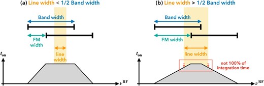
Schematic diagram of the requirements of the spectrometer’s bandwidth for spectral line observation. The top black bars show the bandwidth of a spectrometer with frequency modulation. The bottom graphs show total on-source time achieved with a zigzag FM pattern as a function of the observed RF frequency. (a) The case where the line width |$<$| 1/2 bandwidth: all the samples of a timestream fully cover the line width (FWHM) and sensitivity loss does not occur. (b) The case where the line width |$>$| 1/2 bandwidth: some samples of a timestream do not cover the line width (FWHM), and sensitivity loss occurs at the edges of the line. (Color online)
We note that such sensitivity loss may not affect the band center much because it is only proportional to the square root of the total on-source time, even though on-source time itself drops linearly if we use a zigzag FM pattern. We also note that this is not the case with a spectral line survey, which obtains a frequency range of several GHz over the instantaneous bandwidth of a spectrometer. In this case, we can set the FM width to be wider than half of the bandwidth, which may be an efficient way to conduct the survey compared to conducting PSW observations several times by changing the center frequencies.
5.2 FMLO method in more generalized cases
5.2.1 Modeling atmospheric line emission
5.2.2 FM-dependent gain correction
The conventional non-FM position-switching method assumes that the gain, |${\boldsymbol G}$| (also known as bandpass), does not change between the on-point and hot load measurements (i.e., |${\boldsymbol G}^{\rm on}\simeq {\boldsymbol G}^{\rm load}$|). In the FMLO method, however, the timestream of the on-point gain is modulated and thus has a dependence on the observed frequencies, as mentioned in subsection 4.3. Before the absolute intensity calibration is performed, it is necessary to estimate the FM-dependent gain, |${\boldsymbol G}^{\rm FM}$|, and to separate it from |${\boldsymbol G}^{\rm on}$| to obtain the FM-independent bandpass. In order to correct for the FM-dependent gain, we have two strategies:
To obtain a timestream of the on-point with the FMLO method and a non-FM spectrum of the hot load (the method we adopt in this paper). The FM-dependent gain is then estimated from the on-point timestream itself by smoothing the FM-dependent gain curve (as an analogy of self-calibration in an interferometric observation).
To obtain the timestreams of both the on-point and hot load. The FM-dependent gain is then estimated from the hot load measurements.
In FMLO observations with the TZ receiver, the period of the gain curve is |${\sim } 250$| MHz, which is comparable to the typical line width of extragalaxies (FWHM |$\sim 500$| km s|$^{-1}$|). If we observe such targets, the latter method would be essential to distinguish the FM-dependent gain from the signal. We will discuss both strategies using the observed FMLO data with the FOREST receiver in the next study.
5.3 Improvement of sensitivity and efficiency
5.3.1 Effect of correlated component removal
In subsection 4.4 we demonstrated that PCA properly estimates correlated components, and a cleaned timestream can be obtained after such components are subtracted. There exists, however, an important issue regarding the contribution of noise from the correlated components themselves, which is expressed as the factor |$\alpha _{\rm FMLO}\simeq 1.1$|. Although it is smaller than the factor of position switching (|$\alpha _{\rm PSW}=\sqrt{2}$|), it would be better to minimize such a contribution (i.e., |$\alpha _{\rm FMLO}\rightarrow 1$|). One possible solution is smoothing the correlated components. Bailey (2012) discusses the possibility of “smoothed EMPCA,” i.e., smoothing the basis vectors at each estimation step, and concludes that, compared to the smoothing of noisy eigenvectors, it will result in optimal smooth eigenvectors. This, however, requires that the length scale of the intrinsic correlated components be larger than that of the noise, i.e., the correlated component should have a regular rather than a random spectral shape during an observation. For such an approach, we should obtain data from different observation seasons to monitor the robustness of the modes of correlated components. We may also derive an optimal window length for smoothing using the strategy of smoothed bandpass calibration (Yamaki et al. 2012).
5.3.2 Optimization of the modulation frequency
We use the modulation frequency (|$=$| dump rate of a spectrometer) of 10 Hz throughout the study. While it is determined by an estimate of the timescale of sky variation, the PSD plot in figure 9 suggests that correlated noise dominates at lower frequencies than 0.1 Hz in the case of the Nobeyama |$45\:$|m telescope. As the dwell time of a frequency sweep is fixed (subsection 3.1), the observation efficiency of FMLO would improve with a lower dump rate (for example, |$\eta _{\rm obs}^{\rm FMLO}$| is 0.984 if the dump rate is 2 Hz, which results in |$\sim$|7% improvement). On the other hand, as also shown in the PSD plot, the existance of periodic vibration higher than 1 Hz should also be considered, otherwise it may worsen the sensitivity. The choice of the modulation frequency is therefore a trade-off. The optimization of it for a telescope will be discussed in the next study.
5.3.3 Application to large mapping observations
In subsection 4.6 we demonstrated that the sensitivity improvement of the FMLO mapping is |$\iota \sim 1.1$| (10% improvement) compared to OTF, which seems to be quite small in the case of a single-pointed observation of the FMLO method (|$\iota \sim 1.7$|). This is because, while the on-point observation of the FMLO is 20%–30% more efficient, the noise contribution from the off-point, |$\alpha _{\rm FMLO}$|, is 5% worse than from the OTF. If |$\alpha _{\rm FMLO}$| does not increase, |$\alpha _{\rm OTF}/\alpha _{\rm FMLO}$| worsens (less than unity) for a wider mapping area such as several square-degree surveys. It is, however, expected that we will still obtain a better |$\iota$| for a wider mapping area because there exists an upper limit on the scan length, |$l_{1}$|, of an OTF mapping observation owing to the upper limit of the observed time per scan, |$t_{\rm scan}$|, while an FMLO observation has no such limit. According to “OTF Observations with the |$45\:$|m Telescope” from the Nobeyama |$45\:$|m website,10|$t_{\rm scan}$| should be 10–30 s and an off-point observation should be performed every 10–30 s for a mapping observation of the Nobeyama |$45\:$|m because (1) a larger time interval between off-points causes a baseline wiggle similar to that observed with the PSW method, and (2) a longer |$t_{\rm scan}$| (i.e., longer observation time of an entire map) no longer guarantees the uniformity of a map.
Furthermore, there exists a lower limit for the scan speed, |$v_{\rm scan}$|, where the spatial sampling interval should be |$1/3$|–|$1/4$| of the beam size (HPBW). For a 115 GHz observation of the CO (1–0) line (a beam size of |$15^{\prime \prime }$|) using the Nobeyama |$45\:$|m, for example, |$v_{\rm scan}$| should be 50–60 arcsec s|$^{-1}$|, which yields an upper limit of |$l_{1}= 1000^{\prime \prime }$|–|$1200^{\prime \prime }$|. If we conduct a |$1\times 1$| degree|$^{2}$| mapping observation using both the OTF and FMLO methods, for the OTF method it is necessary to split the mapping area into nine different |$20\times 20$| arcmin|$^{2}$| subregions. This yields an observation efficiency of |$\eta _{\rm obs}^{\rm map}=0.31$|, while the FMLO achieves |$\eta _{\rm obs}^{\rm map}=0.81$|, a much higher value if we use the parameters described in table 1. Together with the noise contribution factor, the sensitivity improvement is |$\iota =1.45$| (45% improvement) and the efficiency improvement per unit noise level is |$\iota ^{2}=2.10$| (110% improvement). This is because we assume that the FMLO mapping can break the upper limit of |$t_{\rm scan}$| and sweep a scan length of |$1^{\circ }$| at a time (|$t_{\rm scan}=72$| s). We note that the derived |$\iota$| is a lower limit. In actual observations, we expect that the baseline wiggles and/or scanning effects are subtracted by correlated component removal, which will result in a much higher |$\iota$| and thus guarantees the uniformity of a map with an even longer scan length.
5.4 Computation cost for data reduction
In a data reduction of the FMLO method, estimating correlated components by PCA takes a large amount of time. A standard PCA requires a computation cost of |$\mathcal {O}[\min (N^{3}, D^{3})]$|, where |$\mathcal {O}$| is big O notation to express the order of a function. If one needs to obtain only the first |$K$| correlated components by singular value decomposition (SVD), the cost would be reduced to |$\mathcal {O} [\min (ND^{2}, N^{2}D)]$|. The typical size of a timestream in the study is |$N=600$|, |$D=2048$|. For the first five correlated components (|$K=10$|), an estimate takes |$\sim$|220 ms (using Mac Pro Late 2013 with 3.5 GHz 6-core Intel Xeon E5). Including any overheads such as loading data and other data reduction steps, the total reduction time of the single-pointed observation of IRC |$+$|10216 (subsection 4.5) was |$\sim$|20 s with 16 iterations. The total reduction time of the mapping observation of Orion KL (subsection 4.6) is much longer than that of IRC +10216; the data size is thirty times larger (|$N\sim 12000$|) and the cube-making takes a much longer time than the spectrum-making. As a result, the total reduction time of a map with a scan pattern was |$\sim$|7 min with 9 iterations and 20 time chunks.
We note that some digital spectrometers already have |$D>10^{4}$| channels (e.g., XFFTS: Klein et al. 2012; PolariS: Mizuno et al. 2014), where correlated component removal becomes time consuming. In such cases, EMPCA would also be a good solution to reduce the computation cost. According to Bailey (2012), the computation cost of EMPCA is |$\mathcal {O}(MNK^3+MNKD)$|, where |$M$| is the number of iterations within an EM algorithm (not iterations of a data reduction procedure). With the number of channels of XFFTS (|$D=2^{15}$|) and a typical iteration time of |$M=10^{2}$|, the computation cost of EMPCA is much smaller than that of PCA by about two orders of magnitude. The reduction of the computation cost by EMPCA will be demonstrated in the next study.
6 Conclusions
In this paper we propose a new observing method for millimeter and submillimeter spectroscopy to achieve high observation efficiency (|$\eta _{\rm obs}>0.9$|) and baseline stability based on a correlated noise removal technique. FMLO, our proposed method, employs spectral correlation of sky emission for instantaneous removal of the emission on a timestream, while astronomical signals are frequency modulated by an LO whose frequency is fast swept (|$\sim$|10 Hz). The conclusions are as follows:
We show that the correlated noise removal technique used in continuum imaging and CMB experiments can be applied to (sub-)millimeter spectroscopy by frequency modulation of a spectral band, which is realized by an FMLO.
We establish the principle of the FMLO method by introducing a mathematical expression of a timestream and its modulation and demodulation. As a specific advantage of the FMLO method, we also express the software-based sideband separation as a result of reverse demodulation of a timestream.
We develop an FMLO observing system and install it on the TZ front-end receiver of the Nobeyama |$45\:$|m telescope. We achieve accurate time synchronization between the telescope’s 1 pps clock and frequency modulation of a digital signal generator that generates the first LO signal of the TZ.
We develop a software-based data reduction procedure for the FMLO method, which employs PCA for the correlated noise removal and an iterative algorithm for accurate estimation of both correlated components and astronomical signals in a timestream.
We conduct single-pointed and mapping observations of Galactic sources with both the FMLO and PSW methods. We demonstrate that the observation efficiency of the FMLO method is dramatically higher than the PSW method: it is at least 3.0 times and 1.2 times better in single-pointed observations and mapping observations, respectively, while the obtained intensities of spectra or maps are consistent between the two methods. The efficiency of the mapping observation could be improved in a larger-scale (|$\sim$|deg|$^{2}$|) mapping, based on our calculation of mapping design.
We find that the estimated correlated components contribute noise to a cleaned timestream, although it is a small contribution compared with that of an off-point measurement. We also have to consider the effect of atmospheric line emission in some observing frequencies. It will be necessary to introduce the weighted PCA method so that correlated components can be smoothed or the atmospheric line emission deweighted, which will be further investigated in the next study.
Acknowledgements
We thank the anonymous referee for fruitful comments. We thank Prof. M. Saito, Assoc. prof. S. Asayama, and Dr. Y. Tatamitani for great support to the FMLO project including implementation and commissioning of the system. This work is supported by KAKENHI (Nos. 23840007, 25103503, 15H02073, 17H06130, and 15J05101). This paper makes use of data taken by the Nobeyama |$45\:$|m radio telescope. The Nobeyama |$45\:$|m radio telescope is operated by the Nobeyama Radio Observatory, a branch of the National Astronomical Observatory of Japan. We made use of SciPy,11 NumPy (Van der Walt et al. 2011), xarray (Hoyer & Hamman 2017), Numba (Lam et al. 2015), scikit-learn (Pedregosa et al. 2011), Astropy (Astropy Collaboration 2013, 2018), and matplotlib (Hunter 2007) for the development of FMFlow. We made use of CASA (McMullin et al. 2007) for making integrated intensity maps and spectra of both OTF and FMLO mapping observations.
Footnotes
We hereafter use the term “single-pointed” when a telescope tracks a celestial coordinates (i.e., an observation of a point-like source). In contrast to single-pointed, the term “mapping” is used when a telescope scans a certain region.
We hereafter define the term “on-point” as the celestial coordinates of an astronomical source and “off-point” as those without any sources.
Hereafter, a symbol with a tilde denotes a demodulated variable.
Hereafter, a symbol with a superscript of i denotes a variable of the image sideband.
Hereafter, an equations like |$\boldsymbol {X}^{\rm (,i)}=\boldsymbol {Y}^{\rm (,i)}+{\boldsymbol Z}^{\rm (,i)}$| bundles two equations for the signal and image sidebands (i.e., |$\boldsymbol {X}=\boldsymbol {Y}+{\boldsymbol Z}$| and |$\boldsymbol {X}^{\rm i}=\boldsymbol {Y}^{\rm i}+{\boldsymbol Z}^{\rm i}$|, respectively).
〈https://github.com/fmlo-dev/fmflow〉 (doi: 10.5281/zenodo.3433962).
Hereafter, a symbol with a hat denotes a variable of an estimate.
Here, “model” does not mean to obtain an estimate of the true value; rather, it means to make a best-effort and noise-free one at each iteration to be used for the next one.
The Frobenius norm of a matrix, |$|\boldsymbol {X}|_{\rm F}$|, is defined as |$|\boldsymbol {X}|_{\rm F} \equiv \left({\sum _{d=1}^{D}\sum _{n=1}^{N}X_{dn}^{2}}\right)^{1/2}$|.
Jones et al. 2001, Scipy: Open Source Scientific Tools for Python 〈https://www.scipy.org〉.
References
