


Abstract
Structures of X-ray emitting magnetic polar regions on neutron stars in X-ray pulsars are studied in the accretion rate range 1017 g s−1–1018 g s−1. It is shown that a thin but tall, radiation-energy-dominated, X-ray emitting polar cone appears at each of the polar regions. The height of the polar cone is several times as large as the neutron star radius. The energy gain due to the gravity of the neutron star in the polar cone exceeds the energy loss due to photon diffusion in the azimuthal direction of the cone, and a significant amount of energy is advected to the neutron star surface. Then, the radiation energy carried with the flow should become large enough for the radiation pressure to overcome the magnetic pressure at the bottom of the cone. As a result, the matter should expand in the tangential direction along the neutron star surface, dragging the magnetic lines of force, and form a mound-like structure. The advected energy to the bottom of the cone should finally be radiated away from the surface of the polar mound and the matter should be settled on the neutron star surface there. From such configurations, we can expect an X-ray spectrum composed of a multi-color blackbody spectrum from the polar cone region and a quasi-single blackbody spectrum from the polar mound region. These spectral properties agree with observations. A combination of a fairly sharp pencil beam and a broad fan beam is expected from the polar cone region, while a broad pencil beam is expected from the polar mound region. With these X-ray beam properties, basic patterns of pulse profiles of X-ray pulsars can be explained too.
1 Introduction
Soon after periodic X-ray variations were discovered from Cen X-3 (Giacconi et al. 1971) and Her X-1 (Tananbaum et al. 1972), accretion environments of such sources were theoretically discussed by Pringle and Rees (1972) and Lamb, Pethick, and Pines (1973). Since then, a large number of X-ray pulsars have been found and theoretical attempts have continuously been being done to explain the observational appearances of X-ray pulsars. We now have a general consensus on the situations of X-ray pulsars, the settings of which could sequentially be summarized as follows:
(1) a close binary of a strongly magnetized neutron star + a “normal” companion star,
(2) an accretion flow from the companion star to the neutron star,
(3) a magneto-boundary surface at ∼108 cm from the neutron star where the magnetic pressure stops the accretion flow,
(4) two channeled flows along magnetic funnels towards the magnetic poles on the neutron star surface,
(5) very hot regions at the bottoms of the channeled flows, after energy conversions of the kinetic energies to thermal energies through standing shocks,
(6) X-ray emissions from the polar regions near the neutron star surface,
(7) an oblique rotation of the magnetic axis, causing X-ray pulsations.
Pioneer studies on the properties of the X-ray emitting regions had already done by some authors by the mid-1970s. Davidson (1973) proposed a situation that a hot, dense mound should be formed above each magnetic pole and that infalling material would be decelerated by the radiation pressure of photons trapped inside the mound. He further argued that energy released above the mound should diffuse out as moderately hard X-rays and that energy released within the mound should emerge as soft X-rays from the whole surface of the neutron star. By extending the idea of the radiation-pressure dominant polar mound to cases of high accretion rate, Inoue (1975) studied a structure of a radiation-pressure dominant polar cone above each magnetic pole by taking account of the effect of the gravity there. He discussed that the gravitational energy released in the polar cone should be radiated away from the surface of the cone as a multi-color blackbody emission. Basko and Sunyaev (1975), on the other hand, discussed the generation and diffusion of radiation in a plasma with a strong magnetic field at the bottom of a magnetic funnel, supposing a fairly low accretion rate corresponding to the X-ray luminosity ≪1037 erg s−1.
Even at this early stage in the middle of 1970’s, a general picture of X-ray emission regions on each magnetic pole of X-ray pulsars was suggested. It was that two regions should exist; the primary region where the kinematic energy of the infalling matter is converted to thermal energy and photons generated there or from the bottom side diffuse out upward suffering various interactions with matter in a magnetized plasma, and the secondary region where the accreted matter still gradually falls, being braked by the radiation pressure, and the gravitational energy gained there finally diffuses out from its surface and/or the adjacent neutron star surface as blackbody emissions. Studies on the primary region have since been done by several authors (e.g., Becker & Wolff 2007; Wolff et al. 2016) but the secondary region has not been studied in more detail than by the work of Inoue (1975).
In this paper, we study the nature and structure of the secondary region as a function of |$\dot{M}$| more precisely than such simple arguments given above. Based on the results, we then discuss observational appearances of X-ray emissions from there, focusing on cases of fairly high accretion rates corresponding to X-ray luminosities of 1037–1038 erg s−1. In section 2, the basic assumptions of studying the accretion flow along the magnetic funnel are presented and structures of the X-ray emitting regions around the magnetic pole are solved through approximate equations. In section 3, we discuss observational appearances of X-ray spectra and pulse profiles expected from the magnetic polar regions as studied in section 2. Summary and discussions are given in section 4.
2 Structures of magnetic polar regions
2.1 Magneto-boundary surface
Following the general consensus summarized in the previous section, we consider a situation that matter flows from a companion star into a region governed by the gravitational field of a neutron star with magnetic field as strong as 1012–1013 gauss at its surface. The magnetic field halts the matter from further falling around the magneto-boundary surface at the distance ∼108 cm from the neutron star. The matter then flows along the magneto-boundary surface towards the magnetic poler regions and falls on to the neutron star through two funnel-like tubes guided by the magnetic lines of force.
The picture of the magneto-boundary surface was historically first studied in the case of roughly spherical accretion by a strongly magnetized compact star (e.g., Lamb et al. 1973; Inoue & Hōshi 1975; Arons & Lea 1976; Elsner & Lamb 1977), where the magnetic field is considered to be confined inside the magneto-spheric cavity as a result of complete screening of the stellar magnetic field from the outside plasma by currents in the transition region between the magneto-boundary surface and the plasma.
In the case that a thin disk extends down to the magneto-bounding surface, which should be more realistic in most of X-ray pulsars than the spherical flow, the accretion flow from the disk to the neutron star surface was studied in detail by Ghosh, Lamb, and Pethick (1977) and Ghosh and Lamb (1978, 1979). It is shown that the stellar magnetic field penetrates the inner part of the disk through the Kelvin–Helmholtz instability, turbulent diffusion, and so on, and that a transition zone arises in which magnetic coupling between the star and the disk transfers the angular momentum from the disk to the star. The accreted matter is thus considered to flow from the innermost region of the disk along the lines of force of the stellar magnetic field on to the polar regions of the stellar surface by getting over the barrier of the centrifugal force through the angular momentum transfer.
In the scheme of Ghosh and Lamb (1978, 1979), only a thin disk is assumed to extend down to the magneto-boundary region and |$\sim 20\%$| of the stellar magnetic field is considered to remain outside the inner edge of the disk. Recent observations, however, indicate that a geometrically thick flow could exist in parallel to the thin disk from the outermost part of the accretion disk (Churazov et al. 2001; Sugimoto et al. 2016; H. Inoue in preparation). If so, the thick flow should completely screen the remaining magnetic field and thus such a configuration as is seen in figure 1 could be expected. As discussed by Ghosh and Lamb (1978, 1979), a fraction of the magnetic field should penetrate the inner part of the thin disk and the matter should flow along the lines of force of the field threaded in the disk by losing its angular momentum through the magnetic stress force. A small fraction of the magnetic field could remain outside the transition layer in which the matter is flowing from the thin disk but it should completely be compressed and screened by the plasma in the thick disk. The matter in the thick disk could go into the transition layer through instabilities such as the Reyleigh–Taylor instability (Arons & Lea 1976; Elsner & Lamb 1977), and flow together with the matter from the thick disk on to the neutron star surface. As a result, the outer surface of the transition layer could have a shape similar to those obtained by Arons and Lea (1976) and Elsner and Lamb (1977), as schematically drawn in figure 1, where two cusps appear on the magnetic axis. Here, we assume for simplicity that the magnetic axis and the rotational axis of the neutron star are aligned with each other and are perpendicular to the disk plane, as is done in the above literatures.
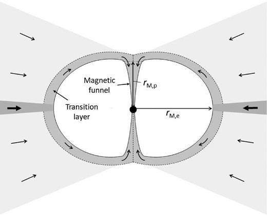
Schematic cross-section of the magneto-boundary surface considered in this paper.
2.2 Overall picture of the magnetic polar regions
As the matter falling in the magnetic funnel finally hits the neutron star surface, a standing shock should appear at a certain height from the stellar surface. The matter can be approximated to flow with the free-fall velocity on the upper-stream side of the shock. We call this region the free-fall region.
The kinetic energy of the inflowing matter should be converted to the thermal energy through the shock. Thermal emissions are expected mainly in the X-ray band from the region between the shock and the stellar surface. We call this X-ray emitting region the polar cone. The thermal pressure is lower than the magnetic pressure in the polar cone, and the matter falls inwards along the magnetic lines of force there.
At the bottom of the polar cone, however, the matter pressure comes to exceed the magnetic pressure and the matter flows out along the stellar surface from the polar cone by dragging the magnetic lines of force. A mound-like structure appears at each of the two polar surface regions and additional X-ray emissions are expected from there. We call these mound-like structures the polar mounds hereafter.
Figure 2 shows the schematic diagram of the magnetic polar regions considered in this paper.
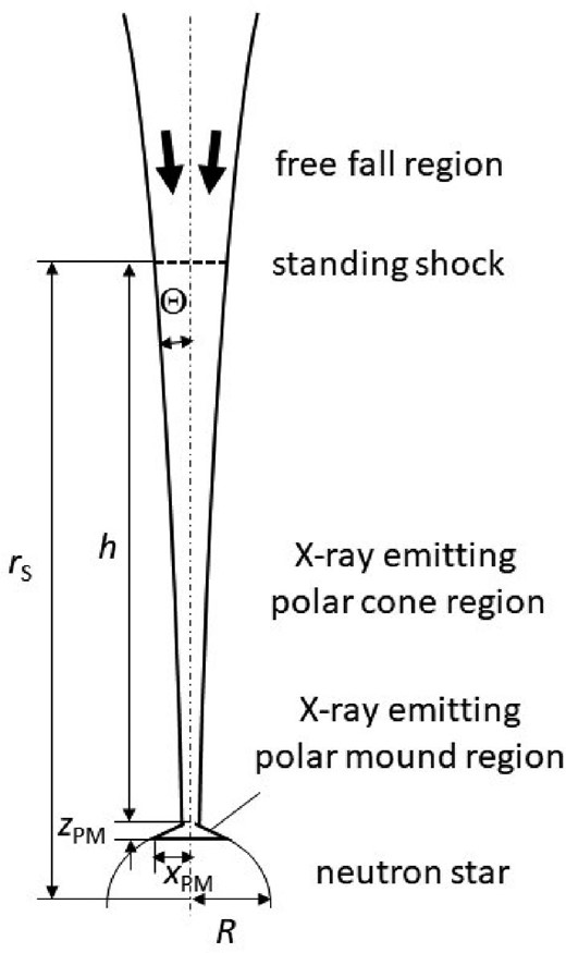
Schematic diagram of magnetic polar regions considered in this paper.
2.3 Free-fall region
2.4 X-ray emitting polar cone region
2.4.1 Dominance of the radiation energy in the polar cone
As shown in equation (25), the optical depth is larger than unity even in the free-fall region in front of the shock. The density behind the shock front must be larger than the density in the free-fall region and the density gets larger and larger as the matter infalls in the polar cone. Thus, we can say that polar cone is sufficiently optically thick.
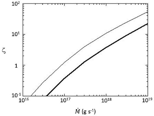
ζ-value, which indicates the dominance of the radiation energy density behind the shock, as a function of |$\dot{M}$|. The thick and thin lines correspond to cases of μM = 1030 gauss cm3 and μM = 1031 gauss cm3, respectively.
2.4.2 Energy loss due to side-say diffusion of photons
2.4.3 Structure of the polar cone
Based on the above arguments, equations determining structures of the polar cone are as follows.
The first is the continuity equation which is given in equation (23) by replacing |$v$|T with |$v$|. Here, we assume for simplicity that ρ and |$v$| are uniform on a cross-section in the azimuthal direction of the polar cone.
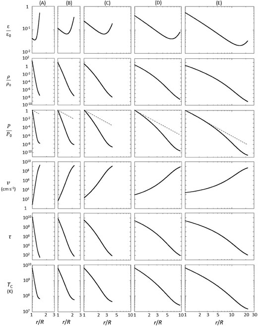
Solutions of equations (42) and (43) have been found with the procedures described above in various cases of |$\dot{M}$|, where we have adopted M = M|$_{\odot}$|, R = 106 cm and two cases of Br,* as 1012 G and 1013 G. The obtained ϵ, ρ, P, |$v$|, τ, and TC as functions of r are shown for five cases of |$\dot{M}$| for Br,* = 1012 G in figure 4 and for Br,* = 1013 G in figure 5, respectively. Here, |$v$| has been calculated from the continuity equation. τ is the optical depth for the Thomson scattering in the tangential direction of the polar cone. TC is the typical temperature of the matter in the polar cone and has been calculated by an equation as TC = (ρ ϵ/a)1/4, where a is the first radiation constant. The normalization parameters in the figures are defined as ϵ0 = GM/R, |$\rho _{0} = 3 B_{\rm r, *}^{2} R / (8 \pi GM) \sim 9 \times 10^{2} (B_{\rm r, *}/10^{12}\:$|G)2(M/M|$_{\odot}$|)−1(R/106 cm) g cm−3, and P0 = P* in equation (45).
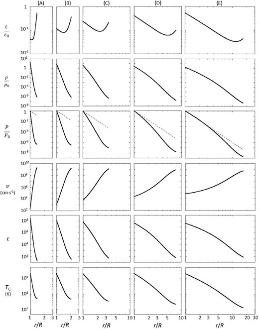
Solved distributions of ϵ, ρ, P, |$v$|, τ, and TC as functions of r in five |$\dot{M}$| cases for Br, * = 1012 G. Columns (A), (B), (C), (D), and (E) correspond to cases of |$\dot{M} = 3 \times 10^{16}\:$|g s−1, 1017 g s−1, 3 × 10¹⁷ g s−1, 1018 g s−1, and 3 × 10¹⁸ g s−1, respectively. Dashed lines in the row of P represent the r-dependence of the magnetic pressure as ∝ r−6.
Same as figure 4 but for Br,* = 1013 G.
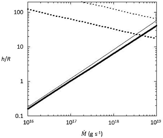
Height of the polar cone region as a function of |$\dot{M}$| (solid lines). Dotted lines indicate positions of rM,p. The thick and thin lines correspond to cases of Br,* = 1012 G and 1013 G. respectively.
2.4.4 Energy loss from the polar cone
From figures 4 and 5, we see, irrespectively of |$\dot{M}$|, that ϵ decreases as r decreases from rS but that it increases after r gets smaller than a certain value. The variation of ϵ is determined by equation (42), in which the first term and the second term on the right-hand side are the energy loss rate through the radiative diffusion and the energy gain rate from the gravitational energy, respectively. In the upper region near the shock, the radiative cooling rate is dominant compared to the energy gain rate and ϵ decreases as the matter flows downwards. The energy gain rate through the gravitational acceleration, however, becomes dominant compared to the energy-loss rate and ϵ starts increasing with r-decrease when r gets smaller than the boundary distance, rB, where dϵ/dr = 0. Hereafter, the region where r > rB and that where r < rB are called as the upper polar cone region and the lower polar cone region respectively.
Figure 7 shows respective portions of the three amounts of the energy |$w$|U, |$w$|L, and |$w$|* to the sum of the three, as functions of |$\dot{M}$| in the case of Br,* = 1012 G. The result is about the same in the case of Br,* = 1013 G. We see that |$w$|H is dominant when |$\dot{M} \lesssim 10^{17}\:$|g s−1, the three are comparable to one another when 1017 g s−1|$\lesssim \dot{M} \lesssim 10^{18}\:$|g s−1, and |$w$|* is dominant when |$\dot{M} \gtrsim 10^{18}\:$|g s−1.
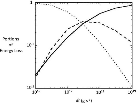
Portions of energy loss in the upper polar cone region (dotted line), the lower polar cone region (dashed line) and in the mound region (thick line) as functions of |$\dot{M}$| in the case of Br,* = 1012 G.
2.5 X-ray emitting polar mound region
The accreted matter still tends to flow downwards with a significant amount of the thermal energy at the bottom of the polar cone, but the thermal pressure should get stronger than the magnetic pressure of the surrounding magnetic funnel if the matter flows further below the bottom boundary. Thus, the matter should start expanding along the surface of neutron star, dragging the magnetic lines of force. We call this tangentially expanding region the polar mound region. The schematic cross-section of the polar mound is drawn in figure 8.
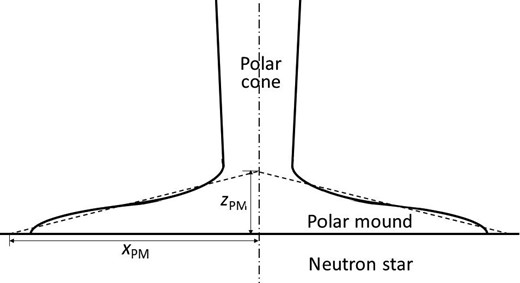
Schematic cross-section of the polar mound. The shape is approximated by a low cone, as indicated with dashed lines, with a radius xPM of the base and a height |$z$|PM at the center, in order to roughly estimate the sizes of the polar mound.
The structure of the polar mound should be determined from the following two conditions.
By seeing α from the P distribution in the polar cone as a function of |$\dot{M}$|, shown in figures 4 and 5, and solving simultaneous equations (55) and (59), we obtain xPM and |$z$|PM as functions of |$\dot{M}$| in two cases of B*. The results in the case of B* = 1012 gauss are plotted in figure 9. Those in the case of B* = 1013 gauss are almost identical. When |$\dot{M}$| becomes larger than 1018 g s−1, xPM comes to be as large as or even larger than R and simple arguments as done above become inapplicable.
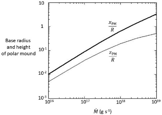
Base radius (the thick line) and height (the thin line) of the polar mound, in units of stellar radius, as a function of |$\dot{M}$|.
3 X-ray emissions from the magnetic polar regions
We have seen the portions of energy loss from the upper polar cone region, the lower polar cone region, and the polar mound region in sub-subsection 2.4.4. Since the energy lost from these regions should be emitted mainly in X-rays from their surfaces, the portions of the energy loss from the three regions as shown in figure 7 correspond to those of the local X-ray luminosities.
As seen in the top panels of figures 4 and 5, two local maxima of ϵ appear, and the locally most luminous positions in the polar cone are the top of the polar cone just behind the shock and the bottom of the polar cone just on the neutron star surface. The most luminous place, however, depends on |$\dot{M}$|. When |$\dot{M} \lesssim 10^{17}\:$|g s−1, the top of the polar cone is the most luminous, when |$\dot{M} \simeq 3 \times 10^{17}\:$|g s−1, the top and the bottom of the polar cone are comparably luminous, and when |$\dot{M} \gtrsim 10^{18}\:$|g s−1, the bottom is the most luminous.
The relative amount of the differential luminosity between the top and bottom of the polar cone is seen to depend on |$\dot{M}$| in figure 7 too. This figure further reminds us that the polar mound region is the most luminous when |$\dot{M} \gtrsim 3 \times 10^{17}\:$|g s−1.
3.1 Properties of X-ray spectrum
When |$\dot{M} \lesssim 10^{17}\:$|g s−1, X-ray emission from the upper polar cone is the most luminous. As seen from the top panels of figures 4 and 5, the logarithmic slope of ϵ against r, ν, is much larger than unity, and thus a single blackbody spectrum is expected in this |$\dot{M}$| range within the simplified arguments in this study. Since the establishment of the radiation field is thought to be insufficient behind the shock as in figure 3, however, Comptonization of bremsstrahlung photons and blackbody photons produced around there should be taken into account to consider properties of X-ray spectrum from there; this was already studied by Becker and Wolff (2007) and Wolff et al. (2016). We do not go into detail on this low-|$\dot{M}$| range here.
When |$\dot{M} \gg 10^{17}\:$|g s−1, on the other hand, the X-ray emissions from the upper polar cone region get less luminous than those from the lower polar cone region and the polar mound region. Furthermore, since the distance of the shock front, rS, is several times as large as the neutron star radius in the case of |$\dot{M} \simeq 10^{18}\:$|g s−1 (see figure 6), the temperature of the emission from the upper polar cone region should be much lower than those from the two regions near the neutron star surface. Thus, we neglect the contribution of the emission from the upper polar cone region here because our present concern focuses on the properties of the X-ray spectrum in the energy range above a few keV in the |$\dot{M}$| range around 1018 g s−1.
From the lower polar cone region, we can expect a multi-color blackbody spectrum, which should be expressed with the p-free disk model (Kubota & Makishima 2004). This model was developed to reproduce X-ray spectra from accretion disks and the surface blackbody temperature is assumed to be distributed as a function of an orbital radius in a disk as in equation (64). In the present case considered here, the p parameter is given by equation (68). The value of ν, which is defined as the logarithmic slope of ϵ against r in equation (65), can be calculated from the radial distribution of ϵ solved in sub-subsection 2.4.3, and is ∼−1.3 near the bottom of the polar cone when |$\dot{M}$| is around 1018 g s−1. Then, p is estimated to be ∼0.7, taking account of η = 0.5 as assumed in equation (20), and we set ω = 0 for simplicity. The highest apparent temperature in the multi-color component can be estimated from equation (63) by setting ϵ = ϵ*, r = R, and Θ = Θ*, and assuming |$\tau _{\rm a}^{1/4} \simeq 2$| (e.g., Shimura & Takahara 1995). Since ϵ* ≃ 0.4ϵ0 when |$\dot{M} = 10^{18}\:$|g s−1, as seen both in figures 4 and 5, we get the highest apparent temperature (∼5 keV) around that accretion rate.
From the polar mound region, a quasi-single blackbody spectrum should be detected. The apparent temperature, Ta,PM, is calculated from equation (70) again to be ∼5 keV when LPM ≃ 1038 erg s−1 and χ−1/4(xPM/R)−1/2 ≃ 2.
According to the above arguments, we can expect a hybrid spectrum composed of the multi-color blackbody spectrum from the lower polar cone region and the quasi-single blackbody spectrum from the polar mound region, for X-ray emissions in the energy range above a few keV, in the case of |$\dot{M} \gg 10^{17}\:$|g s−1.
From these considerations, the fact that an NPEX model consisting of two spectral components—the cut-off power law spectrum and the single blackbody-like spectrum—can reproduce the continuum spectra observed from many X-ray pulsars well could be considered to support strongly the present model, which predicts the presence of two other spectral components, the multi-color blackbody spectrum from the polar cone region and the quasi-single blackbody spectrum from the polar mound region. It should be noted that the temperatures obtained with the NPEX model fits to X-ray spectra observed from several sources by Makishima et al. (1999) are distributed around 5 keV, which agree to the values estimated above in the present study.
Furthermore, K. Kondo, T. Dotani, and H. Inoue (in preparation) have recently analyzed phase-resolved spectra observed from Her X-1 with Suzaku and have successfully resolved the continuum spectra into three components, each of which keeps its respective spectral shape constant and varies only its normalization factor in association with the pulse-phase change, independently of the other components. A remarkable thing is that the two components resolved in the energy range above ∼2 keV are well reproduced with the multi-color blackbody spectrum and the single blackbody spectrum respectively, although they have been obtained in a model-independent way.
3.2 Properties of X-ray pulse profile
Here, we discuss pulse profiles expected from the presently considered configurations in the magnetic polar regions in the case of |$\dot{M} \gg 10^{17}\:$|g s−1.
As seen in figure 12c in Makishima et al. (1999), the crossover energy, where the two components in the NPEX model in equation (71) cross over, generally exists around 10 keV. Thus, we can consider that the multi-color blackbody component, identical to the first component in the NPEX model, from the lower polar cone should mainly govern the pulse profile in an energy range of, say, 2 to 6 or 7 keV. On the other hand, in an energy range above, say, 15 or 20 keV, the single blackbody component, identical to the second component in the NPEX model, from the polar mound region should be the main component in the pulse profile.
We discuss pulse profiles expected for X-rays from the polar cone and the polar mound below. In calculating the pulse profiles, we take into account two effects deforming the profiles; occultation of the emission regions by the neutron star body and influences of relativistic light bending. They are explained in the Appendix.
3.2.1 Directional distributions of X-ray emissions from the polar cone
X-rays from the polar cone mainly form the pulse profile in 2 to 6–7 keV.
Several X-ray pulsars exhibit absorption features at Cyclotron resonance energies around 20–40 keV in their X-ray spectra (e.g., Makishima et al. 1999). Since the X-ray energies of 2 to 6–7 keV now considered are significantly lower than these cyclotron energies, X-rays in this energy range cannot move electrons in the direction perpendicular to the magnetic lines of force. Hence, when X-rays diffuse out in the azimuthal direction of the polar cone, those with a linear polarization perpendicular to the magnetic lines of force (“ordinary photons”) can easily go out of the surface layer without suffering from electron scattering, but those that have another polarization in the direction towards the line of forces (“extraordinary photons”) cannot escape without a number of electron scatterings from the surface layer. Even the extraordinary photons, however, become free from electron scattering, if they are scattered in the direction towards the magnetic lines of force. Therefore, the extraordinary photons should gradually be focused in the direction to the magnetic lines of force through a number of electron scatterings. This beaming effect was first pointed out by Basko and Sunyaev (1975).
3.2.2 Directional distributions of X-ray emissions from the polar mound
X-rays from the polar mound mainly form a pulse profile in the energy range above ∼20 keV.
3.2.3 Expected pulse profiles
The pulse profile of X-rays from the polar cone and the polar mound can be obtained from equation (76) and equation (77), respectively, by substituting φ derived from φ’, which periodically varies in association with the neutron star rotation, taking account of the light-bending effect as shown in the Appendix. φ’ is calculated with an inclination angle, i, of the line of sight to the rotational axis, an angle, θR, of the magnetic axis of the neutron star to the rotational axis, and a rotational angle, ψ, of the magnetic axis around the rotational axis. Figure 10 indicates (A) angular relations among the rotational axis, the magnetic axis, and the line of sight, and (B) a relation between φ and φ’ reflecting the light bending effect. Note that the opening angle of the polar cone and the height of the polar mound are both assumed to be negligibly small in the pulse-profile computations and that all the angular distributions of the emissions from them are given as functions of φ, referring to the magnetic axis.
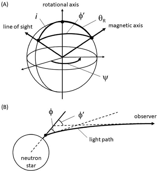
(A) Angular relations among the rotational axis, the magnetic axis and the line of sight, and (B) a relation between φ and φ’ reflecting the light-bending effect.
Figure 11 show two-dimensional distributions of the flux from the polar cone and the polar mound, respectively, as functions of i and ψ, in three cases of θR. Fluxes in figures 11 through 15 are given as fluxes relative to those in cases of isotropic emission, by normalizing dFPC/dr in equation (76) by (dLPC/dr)/(4πD2) for the polar cone component, and FPM in equation (77) by LPM/(4πD2) for the polar mound component, respectively.
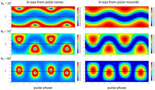
Two-dimensional distributions of flux from the polar cone (left) and the polar mound (right) on pulse phases and inclinations in three cases of θR. ξ = 5, θR = 30°, and φC = 60° are assumed. (Color online)
Since emissions from both the polar cone and the polar mound are mainly focused in the directions of the two magnetic axes corresponding to the N and S poles, two enhancements of the flux appear in each of these maps. In case of emissions from the polar mound, each enhancement has a flux-peak at a position where the line of sight is only directed towards the N or S pole. In the case of those from the polar cone, however, each enhancement has a crator-like hole at its center surrounded by a circular wall with an angular radius of φP as defined in equation (75).
Hereafter, we discuss properties of the pulse profiles only in the range of i ≤ 90° and let the magnetic axis closer to the line of sight be the N pole.
In case of those from the polar mound, pulse profiles in terms of i are somewhat simpler than those of the polar cone. When i is larger than a boundary value, two peaks are exhibited; a stronger peak from the N-pole side and a weaker peak from the S-pole side. When i is smaller than the boundary value, on the other hand, we see only one peak from the N-pole side. The boundary i-value depends on θR and gets larger as θR gets smaller.
The similar trend of the overall flux-enhancements is seen in pulse profiles of X-rays from the polar cone. Sub-peaks, however, appear in some ranges of i in these cases.
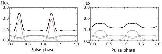
Figure 12 shows some examples of pulse profiles of emissions expected from the present model configurations for different combinations of i and θR. Those of emissions from the polar cone and the polar mound are respectively presented in parallel there. In a relatively soft X-ray band, say, in 2–5 keV, X-rays from the polar cone are dominant, while those from the polar mound are thus in a relatively hard X-ray band, say, in 20–50 keV. Thus, the left- and right-hand panels in figure 12 can be considered to represent pulse profiles expected in the soft and hard bands, respectively.
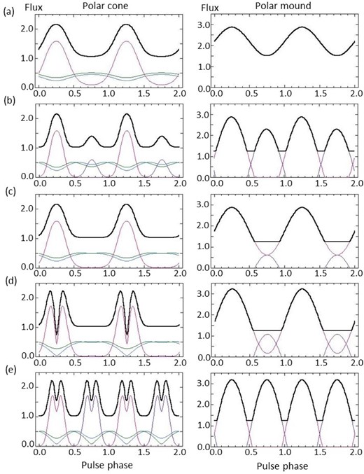
Pulse profiles of fluxes from the polar cone (left) and the polar mound (right) in five cases for the combination of i and θR. (a) through (e) corresponds to cases of (50°, 20°), (80°, 50°), (60°, 30°), (50°, 50°), and (90°, 80°), respectively. If we replace the values of i and θR with each other, the profile is the same. ξ = 5, σE = 30°, and φC = 60° are assumed. The red, purple, blue, and green lines in the polar cone component are profiles of the pencil beam component from the N pole, that from the S pole, the fan-beam component from the N pole, and that from the S pole, respectively. The red and purple lines in the polar mound component are the profiles from the N pole and S pole, respectively. (Color online)
Pulse profiles observed from X-ray pulsars are classified into five groups by Nagase (1989). His classifications are shown (with slight changes to the original wording) as follows:
(a) single sinusoidal-like shapes both in the soft and hard bands,
(b) sinusoidal-like double peaks with little energy dependence, where the amplitudes of the two peaks are usually different,
(c) an asymmetric single peak with some features,
(d) a single sinusoidal-like peak in the high-energy band and close adjacent double peaks in the soft energy band, and
(d) double sinusoidal-like peaks in the high-energy band and complex five peaks in the soft energy band.
Although the sources on which the Nagase’s classifications are based have a wide range of X-ray luminosities, we can assign sources with X-ray luminosities ≳ 1037 erg s−1 to groups (a)–(d); LMC X-4 (e.g., Hung et al. 2010) to (a), SMC X-1 (e.g., Raichur & Paul 2010) to (b), Cen X-3 (e.g., Raichur & Paul 2010) to (c) and Her X-1 (e.g., Deeter et al. 1998) to (d). Vela X-1 (e.g., Makishima et al. 1999) is the representative source of group (e) but its luminosity is as low as ∼1036 erg s−1.
The present model can explain the basic features of the profiles (a) through (d), as seen from figure 12, where each pair of profiles (a) through (d) is shown as a typical example for the respective group (a) through (d). Even for the group (e), we see the presence of multiple peaks in the profile of the polar cone component in figure 12e, although the number of peaks is not five but four.
Even though the pulse profiles are mainly reproduced by adjusting two parameters, θR and i, simultaneous adjusting of the other model parameters should be necessary in order to have the model profile fit to the observed profile as accurately as possible.
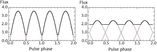
The beam-width parameter, σE, determines the width of the main peak in the pulse profile of the polar cone component. Figure 13 shows the pulse profiles of the polar cone component when we change only the value of σE from 30° to 20° to 40° keeping the other parameters in the case of figure 12c. We can see that the peak profile gets significantly sharper with the σE decrease. In rough comparisons of the models with the observations, σE around 30° seems appropriate.
Examples of pulse profile variations in terms of σE. The pulse profile of the polar cone component in figure 12c in which σE = 30° changes to the left- and right-hand profiles in this figure by replacing σE with 20° and 40°, respectively. (Color online)
The relative distance, ξ, of the X-ray emitting position, normalized by the Schwarzschild radius of the neutron star mass, determines the effects of the relativistic light-bending on pulse profiles. One of the effects appears in the depth of the hollows between pulse peaks of the polar mound component. Figure 14 shows respective pulse profiles of the polar mound component in cases of ξ = 10 and 2.5 when the other parameters are the same as those in figure 12e, in which ξ = 5. We see that the smaller ξ makes the hollow shallower, suffering the larger light bending.
Examples of pulse profile variations in terms of ξ. The pulse profile of the polar cone component in figure 12e in which ξ = 5 changes to the left- and right-hand profiles in this figure by replacing ξ with 10 and 2.5, respectively. (Color online)
The other effect produces small humps between main peaks in combination with the parameter φC, which expresses the degree of the obscuration of X-rays by the neutron star body, defined in the Appendix. Two examples are shown in figures 15. A low plateau begins to appear between two adjacent peaks when we change ξ from 5 to 10 for the profile of the polar cone component in figure 12c, as in figure 15A (left). It gets more significant if we add a change of φC from 60° to 30°, as in figure 15A (right). This feature could explain the presence of a small hump only in the soft band in the observed pulse profile of Cen X-3 (see figure 12 in Raichur & Paul 2009).
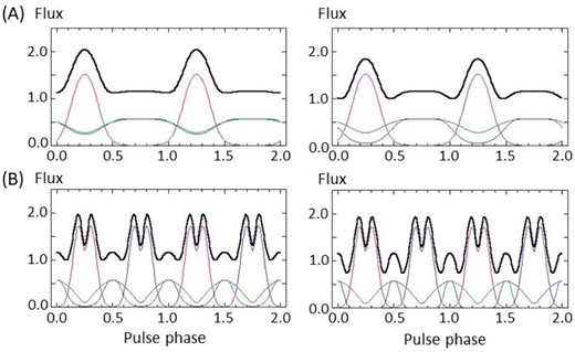
Two examples of pulse profile variations in terms of a combination of ξS and φC. (A) The pulse profile of the polar cone component in figure 12c in which ξ = 5 and φC = 60° changes to the left-hand profile by replacing ξ to 10, and further changes to the right profile by replacing φC to 30°. (B) The pulse profile of the polar cone component in figure 12e in which ξ = 5 and φC = 60° changes to the left- and right-hand profiles by replacing (ξ, φC) to (10, 30°) and further to (10, 15°), respectively. (Color online)
If we change the combination of ξ and φC from (5, 60°) to (10, 30°), the pulse profile of the polar cone component in figure 12e also converts to that of figure 15B (left) and a small peak starts to appear. It gets higher when we further change φC to 15° as seen in figure 15B (right), where we can now present six peaks in the model pulse profile.
As seen above, various combinations of the model parameters can produce variety in the pulse profiles but cannot form an asymmetry of a pulse peak around the center of the peak. Such asymmetries are often seen in observed pulse profiles, and a typical example is the pulse profile of Cen X-3. A similar asymmetry is seen in the pulse profile of Her X-1. It is known, in the case of Her X-1, that the pulse profile changes between the main-on phase and the mid-on phase of the 35-day on–off cycles. Deeter et al. (1998) and Scott, Leahy, and Wilson (2000) propose that the central X-ray emission regions are periodically obscured by the outer boundary of the magnetic funnels located at the inner edge of a precessing accretion disk, and that the pulse phase of the obscuration varies in association with geometry changes due to the disk precession. By introducing such periodic obscuration by the outer boundaries of the magnetic funnels co-rotating with the central neutron star, we could interpret the asymmetries seen in the pulse profiles from Cen X-3 and Her X-1 in the present model frame.
Obscuration could be done even by matter flowing along the magnetic funnels toward the neutron star surface, since the optical depth for the electron scattering of the free-fall region in the magnetic funnel is calculated in equation (25) to be larger than unity unless r ≫ 107 cm. In this case, the obscuration could be observed as an absorption dip in a pulse profile and could interpret some of the features in the complex multiple peaks as seen in the group (e).
4 Summary and discussions
Structures of X-ray emitting magnetic polar regions of neutron stars in X-ray pulsars are studied, and the expected properties of X-ray emissions from them are compared with observations.
The matter flow in the polar cone is solved on several such assumptions as follows:
(1) The flow is one-dimensional in the radial direction, steady and sufficiently subsonic.
(2) The opening angle of the cone is sufficiently smaller than unity and the physical quantities can be represented by respective typical values over the cross-section of the cone.
(3) The optical depth in the tangential direction of the cone is sufficiently large and the radiation energy density is greatly dominant compared to the gaseous one.
(4) The energy loss of the flow is governed by photon diffusion in the tangential direction of the cone.
We discuss the validity of these assumptions below.
Equations (42) and (43) do not include the opening angle parameter, Θ, and thus the solutions on the basic structure of the polar cone do not depend on the assumption of Θ in equation (20). That assumption is necessary only to calculate the inflow velocity and the optical depth in the azimuthal direction.
As seen in figure 6, the height of the polar cone is close to the position of the magneto-boundary surface with the distance of rM,p, when |$\dot{M}$| gets as large as several times 1018 g s−1. Since Θ = 0.32 at rM,p, as obtained in equation (18), Θ ≪ 1 can be assured in the polar cone unless |$\dot{M}$| is close to 1019 g s−1. The solved infall velocities are displayed in figures 4 and 5, while the sound velocities in the polar cones should be 109–1010 cm s−1. These confirm that the flow in the polar cone is sufficiently subsonic. The sufficiently large optical depth can be recognized in figures 4 and 5.
The radiation temperatures of the polar cone are plotted in figures 4 and 5, while the gaseous temperature should be 1011–1012 K in order for the gaseous energy density to comparable to the radiation energy density. Thus we see that the radiation energy is greatly dominant compared to the gaseous one in the polar cone. The establishment of the radiation field just behind the shock front (the upper boundary) has been discussed in sub-subsection 2.4.1.
The temperature at the bottom of the polar cone is simply calculated by the lower boundary condition as |$P = B_{\rm r, *}^{2} / 8\pi$| to be 2.0 × 10⁹ for Br, * = 1012 G, and the average energy of photons is ∼170 keV. Since this energy is much larger than the cyclotron energy, ∼12 keV for Br, * = 1012 G, the reduction of the electron-scattering opacity for photons passing along the magnetic lines’ force should not take place in the main part of the polar cone. Thus, we can say that the simple geometry with Θ ≪ 1 determines the direction of the photon diffusion, which should be the sideways direction.
In practice, however, the term of GM/r on the right-hand side of equation (42) cannot be neglected, and rather plays the more important role with the larger accretion rate. When |$\dot{M}$| is as low as 1016 g s−1, the energy carried with the free-fall matter is almost released soon after the shock. However, when |$\dot{M}$| is as large as 1018 g s−1 or larger, the gravitational energy gain exceeds the energy loss due to the photon diffusion and a significant amount of energy piles up on the bottom side of the polar cone. In section 1 it was mentioned that the presence of the two regions, the primary and secondary regions, were already introduced even in the middle of the 1970s. This paper quantitatively clarifies that X-ray emissions from the primary region is dominant when |$\dot{M} \lesssim 10^{17}\:$|g s−1, and that those from the secondary region become dominant when |$\dot{M}$| exceeds 1017 g s−1.
As the accretion rate increases to 1017–1018 g s−1, the specific radiation energy remaining at the bottom of the polar cone increases. Then, the radiation pressure should increase and exceed the magnetic pressure which holds the flow within the polar cone. As a result, the matter should expand in the tangential direction along the neutron star surface, dragging the magnetic lines of force, and form a mound-like structure (the polar mound region). By assuming that the matter settles on the neutron star surface after losing its remaining energy through photon diffusion in the polar mound and the excess radiation pressure balances with magnetic pressure enhanced by dragging, the structure of the polar mound is simply calculated and the results are reasonable unless |$\dot{M} \gg 10^{18}\:$|g s−1. Davidson (1973) originally introduced the concept of the mound as the optically thick region at the bottom of the magnetic funnel. It is here generalized to be composed of the polar cone and the polar mound, the structures of which vary with the accretion rate.
From such configurations as discussed above, we can expect an X-ray spectrum composed of a multi-color black-body spectrum from the polar cone region and a quasi-single black-body spectrum from the polar mound region from X-ray pulsars with |$\dot{M} \gtrsim 10^{17}\:$|g s−1. These spectral properties basically agree with observations as discussed in subsection 3.1. For further confirmations of the validity of the present model, the following two analyses are expected. One is the analyses of spectral variations linked with the pulse phase, as done by Kondo, Dotani and Inoue (in preparation) for Her X-1. This could resolve the overall spectrum of an X-ray pulsar into several components, which keep a constant spectral shape but change their normalization factors with the pulse phase. The other is to see a spectral change of an X-ray pulsar associated with the flux. The spectrum should get harder as the accretion rate increases, since the relative flux of the quasi-single blackbody component to the multi-color blackbody component increases with the accretion rate.
A fairly sharp pencil beam is expected together with a broad fan beam from the polar cone region, while a broad pencil beam from the polar mound region is expected. With these X-ray beam properties, basic patterns in X-ray pulse profiles observed from X-ray pulsars can be explained too.
The fairly sharp pencil beam is formed when the emitted photon energy is considerably lower than the cyclotron energy at the surface of the pencil beam. The cyclotron energies observed from several X-ray pulsars are around 20 keV (e.g., Makishima et al. 2000), while the typical X-ray energies from the polar cone are around a few keV. This confirms the above condition for the fairly sharp pencil beam to appear. If we see softer X-rays from an X-ray emitting place in the polar cone far from the stellar surface, however, the cyclotron energy rapidly decreases in proportion to r−3 while the surface temperature largely does not. Hence, the beaming effect should tend to weaken in the spectral range below 1 keV.
We have a number of freedoms in the present phenomenological model for the pulse profiles in order to fine-tune the model pulse profile to reproduce an observed pulse profile. In particular, there could be large uncertainties in the periodic obscuration by the outer boundary and the lower side of the free-fall region of the magnetic funnel. The magnetic funnel should be bent in the rotational direction around the axis of the total angular momentum of the accreted matter at the magneto-boundary surface, since the angular momentum should be transferred though the magnetic stress to the neutron star within the magneto-boundary surface. The degree of the bend of the magnetic lines of force depends on the amount of the angular momentum to be transferred (see, e.g., Inoue 1976). Thus, if the amount of the angular momentum changes, the pulse phase at which obscuration by the magnetic funnel takes place should change. In fact, Her X-1 exhibits the pulse-profile change linked with the 35-day on-off cycle. The super-orbital modulation of the X-ray flux can be explained well by the precession of the accretion disk (Inoue 2019). If so, the angular momentum axis of the accreted matter changes with the precession, and the periodic phase-shift of the obscuration place in the pulse profile could be understandable. It could be possible to resolve the practical configurations of the magnetic funnel by changing the model pulse profile to an observed profile.
This model can explain basic features in the pulse-profiles of many X-ray pulsars, as discussed in sub-subsection 3.2.3, but it has not yet been done to show good evidence that the present model can reproduce an observed pulse profile precisely. This should be done in future.
In this paper, we have basically dealt with cases of the accretion rate in the range of 1017–1018 g s−1. In this accretion rate range, we have seen that the fairly tall polar cone stand and the fairly wide polar mound extends from the bottom of the polar cone on each of the magnetic polar regions of the neutron star. The strength of the magnetic field of the neutron star has been assumed to be 1012–1013 gauss at its surface and the obtained configurations of the X-ray emitting polar region do not largely depend on it around this magnetic field range.
When the accretion rate is as low as 1016 g s−1 or less, the height of the polar cone becomes as low as or lower than a tenth of the neutron star radius. Thus, such cases do not fit to the main assumption of the present study that the photon diffusion in the tangential direction plays the main role in constructing the polar cone. Several studies have, however, been done on this low accretion rate case by several authors (e.g., Becker & Wolff 2007; Wolff et al. 2016, and references therein) since the pioneer works of Davidson (1973) and Basko and Sunyaev (1975).
When the accretion rate is as high as 1019 g s−1 or higher, on the other hand, the luminosity largely exceeds the Eddington luminosity of 1 M|$_{\odot}$|. Although the solution can exist in the present scheme of the magnetic polar regions even in the case of |$\dot{M} \simeq 10^{19}\:$|g s−1, some obtained parameters are inconsistent with the approximations in this study.
The first issue is on the base radius of the polar mound, xPM, as shown in figure 9. We see that it exceeds the stellar radius when |$\dot{M}$| gets close to 1019 g s−1. Although this is the result from the very simplified treatment, it could be understood as a tendency for the polar mound to extend over the entire surface of the neutron star as the accretion rate increases. Taking account of the fact that the portion of the energy loss rate from the polar mound gets close to unity when |$\dot{M}$| gets close to 1019 g s−1, as seen in figure 7, most of the super-Eddington luminosity should quasi-spherically be emitted from the entire surface of the neutron star with this accretion rate. It could, therefore, be difficult for the polar mound to maintain the steady state under the super-Eddington radiation pressure. The effect of the radiation pressure might, however, be weakened due to the reduction of the Thomson scattering cross-section under the strong magnetic field on the surface of the neutron star.
The second issue is on the height of polar cone. It becomes as high as or higher than that of the magneto-boundary surface when |$\dot{M} \gtrsim 10^{19}\:$|g s−1, as shown in figure 6. If the upper boundary of the polar cone reaches the magneto-boundary surface, the matter trying to flow into the magnetic funnel should flood over the magneto-boundary surface. In that case, the approximations around the upper boundary of the polar cone in the present study become inapplicable and we will need some new treatments for them.
This estimation is, however, made on the assumption that the magnetic axis aligns with the rotational axis of the neutron star and both axes are perpendicular to the equatorial plane of the accretion disk. In practical cases of X-ray pulsars, the magnetic axis must be oblique to the rotational axes, and thus the matter distribution in the transition layer should be biased to the equatorial plane of the disk. In those cases, a part of the transition layer could be optically thin and steady accretion, in which the matter inflow and the photon outflow segregate from each other, might be possible even if the luminosity exceeds the Eddington limit.
These issues in the case of |$\dot{M} \gtrsim 10^{19}\:$|g s−1 as discussed above are quite interesting in relation to ultra-luminous X-ray pulsars recently discovered one after another (Bachetti et al. 2014; Fürst et al. 2016; Israel et al. 2017; Carpano et al. 2018), and await future studies.
This study presents several clues to resolve observational evidence of X-ray pulsars from various viewpoints, but is still based on several simplified assumptions and approximations. Further theoretical and observational studies of X-ray pulsars are largely expected.
Acknowledgements
The author greatly appreciates the referee for his or her critical comment on the original manuscript.
Appendix. Deformations of pulse profiles by the central neutron star
We discuss two effects deforming the pulse profile of X-ray pulsars owing to the central neutron star.
Here, φ is an angle, at which the light is emitted from a place with a relative distance, ξ, to the radial direction from the gravity center, and φ′ is an angle at which the light is observed at infinity, to the original radial direction.
References
