


Abstract
We conducted an exploration of 12CO molecular outflows in the Orion A giant molecular cloud to investigate outflow feedback using 12CO (|$J = 1\!-\!0$|) and |${}^{13}$|CO (|$J = 1\!-\!0$|) data obtained by the Nobeyama 45 m telescope. In the region excluding the center of OMC 1, we identified 44 12CO (including 17 newly detected) outflows based on the unbiased and systematic procedure of automatically determining the velocity range of the outflows and separating the cloud and outflow components. The optical depth of the 12CO emission in the detected outflows is estimated to be approximately 5. The total momentum and energy of the outflows, corrected for optical depth, are estimated to be |$1.6 \times 10^{2}\, M_{\odot }\:$|km|$\:$|s|$^{-1}$| and |$1.5\times 10^{46}\:$|erg, respectively. The momentum and energy ejection rate of the outflows are estimated to be 36% and 235% of the momentum and energy dissipation rates of the cloud turbulence, respectively. Furthermore, the ejection rates of the outflows are comparable to those of the expanding molecular shells estimated by Feddersen et al. (2018, ApJ, 862, 121). Cloud turbulence cannot be sustained by the outflows and shells unless the energy conversion efficiency is as high as 20%.
1 Introduction
During the early phase of star formation, molecular outflows are ubiquitous phenomena in both low- and high-mass star-forming regions (e.g., see Lada 1985; Arce et al. 2007). Outflows inject energy and momentum into the parent molecular cloud and may play an important role in the self-regulation of star formation (e.g., see Norman & Silk 1980; Bally 2016). This substantial injected energy can affect the cloud structure and evolution (Solomon et al. 1981). Feedback from outflows may maintain the turbulence in molecular clouds (Shu et al. 1987; Nakamura & Li 2007), protecting the clouds from gravitational collapse (Shu et al. 1987).
In the past decade, many researchers have investigated molecular outflows and their feedback in parent molecular clouds by comparing the energy ejection rates of outflows and the energy dissipation rates of cloud turbulence. For example, Arce et al. (2010) conducted an outflow survey in Perseus and concluded that the outflows had sufficient energy to feed the observed turbulence in the entire Perseus cloud complex (see also Hatchell et al. 2007, 2009). Nakamura et al. (2011a, 2011b) investigated the outflows in the L1688 cloud of the |$\rho$| Ophiuchi regions and the Serpens South cloud, and they found that the energy ejection rate of outflows in each cloud was comparable to the energy dissipation rate of the cloud turbulence (see also White at al. 2015). Li et al. (2015) conducted an unbiased outflow survey in Taurus and concluded that the outflow feedback was sufficient to maintain the observed turbulence in the current epoch. The above-mentioned studies were all conducted in relatively low-mass (|$\le 10^{4}\, M_{\odot }$|; Enoch et al. 2006) molecular clouds containing low-mass star-forming regions. In this study, we investigate the feedback of outflows in the Orion A giant molecular cloud (referred to simply as Orion A hereafter), which contains high-mass star-forming regions.
Orion A is the nearest high-mass star-forming region, with a distance estimated to be |$414 \pm 7\:$|pc by Menten et al. (2007). Orion A is often divided into several subregions (e.g., see Bally 2008; Feddersen et al. 2018). OMC 2/3 is an intermediate-mass star-forming region located in the northernmost part of Orion A (Chini et al. 1997). More than 500 young stellar objects (YSOs) have been found in this region in previous observations (e.g., see Chini et al. 1997 and Megeath et al. 2012). OMC 1 has the brightest intensity and the largest velocity width. This region contains the H ii region M42 created by the Trapezium cluster as well as the BN/KL Nebula. OMC 4/5 is located south of OMC 1. Shimajiri et al. (2015a) identified 225 cores in dust continuum at |$\lambda =1.1\:$|mm in this region. L1641-N and NGC 1999 contain well-known young clusters such as L1641-N and V380 Ori, respectively. Approximately 80 YSOs have been identified in the L1641-N cluster (Fang et al. 2009). The V380 Ori cluster contains many Harbig–Haro (HH) objects (Allen & Davis 2008).
Previous outflow surveys of Orion A were limited to particular subregions, such as OMC 2/3 (e.g., Chini et al. 1997; Aso et al. 2000; Williams et al. 2003; Takahashi et al. 2008; Berné et al. 2014), V380 Ori (Davis et al. 2000), and L1641-N (Stanke & Williams 2007; Nakamura et al. 2012). In particular, the OMC 2/3 regions were observed relatively well. Aso et al. (2000) and Williams et al. (2003) conducted outflow surveys of OMC 2/3 in 12CO (|$J = 1\!-\!0$|) with angular resolutions of |$\sim {20^{\prime \prime }}$| and |$\sim {10^{\prime \prime }}$|, and they identified eight and nine outflows, respectively. Williams et al. (2003) found that the energy ejection rate of the outflows was comparable to the energy dissipation rate of the cloud turbulence in OMC 2/3. Takahashi et al. (2008) also conducted a survey of the same region with 12CO (|$J = 3\!-\!2$|) and detected 14 outflows. They identified outflows from the analyses of channel maps and position–velocity diagrams. Despite their efforts, the search procedures of outflows in these studies were not systematic.
In this paper, we present the results of our systematic outflow survey across the entirety of Orion A cloud and discuss the impact of the outflows on their parent molecular cloud. This work is part of the “Star Formation Legacy Project” using the Nobeyama 45 m telescope; an overview of the project is given in a separate paper (Nakamura et al. 2019). An outline of the remainder of this paper is as follows. Section 2 describes the details of our Nobeyama 45 m observations and data. In section 3, we present a systematic procedure for searching outflows. The results of our outflow search and the physical parameters of the identified outflows are given in section 4. In section 5, we discuss the outflow feedback into Orion A. Section 6 summarizes the main results of this study.
2 Observations and data
We conducted |$2\:$|deg|$^{2}$| mapping observations of 12CO (|$J = 1\!-\!0$|, 115.271202 GHz) and |${}^{13}$|CO (|$J = 1\!-\!0$|, 110.201354 GHz) of Orion A using the FOREST (Minamidani et al. 2016) receiver mounted on the National Radio Observatory (NRO) 45 m telescope. The observations were made between 2014 December and 2017 March. The telescope beam size (HPBW) was |$\sim {14^{\prime \prime }}$| at |$115\:$|GHz and the typical pointing accuracy was |${3^{\prime \prime }}$|. We employed the On-The-Fly (OTF) scan mode (Sawada et al. 2008) for the mapping observations. We adopted a spheroidal function with a spatial grid size of |${7{^{\prime \prime }_{.}}5}$| as a convolution function. To improve sensitivity and coverage, we combined the FOREST data and with previously published data (Shimajiri et al. 2011, 2014, 2015b; Nakamura et al. 2012) collected by the BEARS receiver (Sunada et al. 2000). The final maps of the 12CO and |${}^{13}$|CO have an effective resolutions (FWHM) of |$\sim{22^{\prime \prime }}$|, corresponding to |$\sim 0.05\:$|pc at a distance of |$414\:$|pc, and an effective velocity resolution of |$\sim 0.2\:$|km|$\:$|s|$^{-1}$|. The typical root mean square (rms) noise levels of the 12CO and |${}^{13}$|CO cubes are |$0.47\:$|K and |$0.18\:$|K in units of |$T_{\rm MB}$|, respectively. Table 1 summarizes the observations and data. More details on the observations and data reduction are described by Kong et al. (2018) and Nakamura et al. (2019).
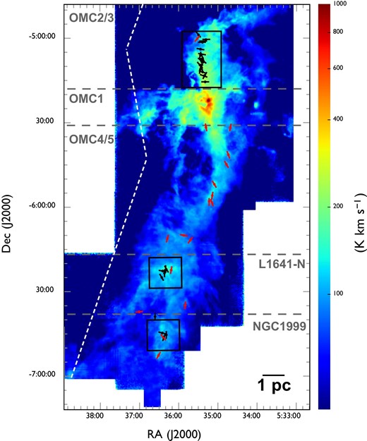
Figures 1 and 2 show the total integrated intensity maps of the 12CO (|$J = 1\!-\!0$|) and |${}^{13}$|CO (|$J = 1\!-\!0$|) emissions of Orion A, respectively. An integral-shaped filament is clearly seen for both 12CO and |${}^{13}$|CO. The averaged line profiles of the 12CO and |${}^{13}$|CO in each subregion are shown in figure 3. The peak velocities of the 12CO and |${}^{13}$|CO spectra in figure 3 shift from |$11\:$|km|$\:$|s|$^{-1}$| to |$8\:$|km|$\:$|s|$^{-1}$| in the north-to-south direction. The averaged velocity widths at OMC 2/3, OMC 1, OMC 4/5, L1641-N, and NGC 1999 are |$3.1,\ 4.7,\ 3.8, 4.0$|, and |$3.3\:$|km|$\:$|s|$^{-1}$| for |$^{12}$|CO and |$2.1,\ 4.0,\ 3.1,\ 3.5$|, and |$2.8\:$|km|$\:$|s|$^{-1}$| for |$^{13}$|CO, respectively. These values are obtained from Gaussian-fitting to each spectrum, as shown in figure 3. More details on the data, including the first and second moment maps and channel maps of the 12CO (|$J = 1\!-\!0$|) and |${}^{13}$|CO (|$J = 1\!-\!0$|), are provided by Kong et al. (2018) and Nakamura et al. (2019).
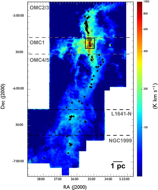
Outflow driving source candidates superposed on the 12CO (|$J = 1\!-\!0$|) total integrated intensity map of Orion A. The integrated velocity ranges from |$2.0\:$|km|$\:$|s|$^{-1}$| to |$20.0\:$|km|$\:$|s|$^{-1}$| in |$v_{\rm LSR}$|. The open circles, filled circles, and filled crosses indicate the positions of the protostars without H|$_2$| jets, protostars with H|$_2$| jets, and pre-main-sequence stars with H|$_2$| jets, respectively (Megeath et al. 2012; Davis et al. 2009). The black square represents the center of OMC 1. (Color online)
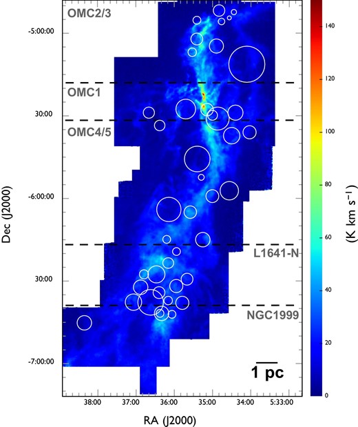
|${}^{13}$|CO total integrated intensity map of Orion A. The integrated velocity ranges from |$2.0\:$|km|$\:$|s|$^{-1}$| to |$20.0\:$|km|$\:$|s|$^{-1}$| in |$v_{\rm LSR}$|. The white circles indicate molecular shells identified by Feddersen et al. (2018). The size of each circle reflects the shell size. (Color online)
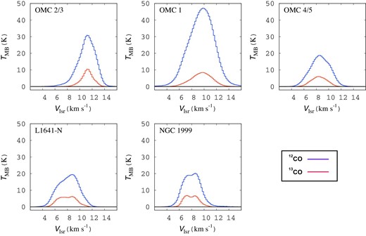
Averaged spectra of 12CO (|$J = 1\!-\!0$|) (blue) and |${}^{13}$|CO (|$J = 1\!-\!0$|) (red) in each subregion. All spectra are presented for emissions detected above |$5\sigma$|. (Color online)
The black square shown in figure 1 is the center of OMC 1 and indicates the area that is excluded from the following analysis because the identification of the outflows there is difficult with our method (see section 3). There are two reasons why we excluded this area from our procedure. (1) YSOs in this region are so crowded that we cannot judge which YSO is responsible for any particular high-velocity component or is a candidate for outflows. (2) The local velocity width of the molecular clouds around each YSO is so broad that we cannot separate the outflow components from the main cloud components.
3 Method for identifying molecular outflows
To investigate the outflow feedback into the parent cloud, we identify the CO outflows and estimate their physical parameters based on the data cube of the 12CO (|$J = 1\!-\!0$|) emission line. In this section, we describe our outflow search procedure.
3.1 Outflow driving source candidates
To identify the molecular outflows in the vicinity of YSOs, we summarize a set of YSO candidates in our observed region. We made a sample of candidate outflow driving sources from the Spitzer YSO catalog produced by Megeath et al. (2012). The YSOs were divided into two categories based on their infrared photometry: protostars and pre-main-sequence (PMS) stars with a circumstellar disk. We selected protostars as candidate driving sources of outflows because outflows tend to appear in an early phase of star formation. In our observed region, Megeath et al. (2012) identified 198 protostars, including 32 protostars in the center of OMC 1.
We also supplemented the candidates with sources that appear to drive H|$_2$| jets. Davis et al. (2009) conducted an unbiased survey of the molecular hydrogen emission line of |$v = 1\!-\!0$| S(1) at |$2.12\, \mu$|m originating from shocks in outflows (see also Stanke et al. 2002). Davis et al. (2009) also identified driving sources of H|$_2$| jets from the Spitzer YSO catalog based on the jets’ morphologies and/or alignments, arguing that 65 YSOs were associated with H|$_2$| jets in our observed region. Among the 65 YSOs, 53 were categorized as protostars and 12 were categorized as PMS stars.
We eventually focused on 178 candidates outflow driving sources selected from Megeath’s catalog, 65 of which Davis described as YSOs associated with jets. Table 2 summarizes the number of candidates in each category, and figure 1 shows all candidate driving sources of the outflows superposed on the 12CO (|$J = 1\!-\!0$|) integrated intensity map.
Observed lines and data sensitivity.
| Molecule | Transition | Rest frequency | Effective resolution | Velocity resolution | Noise level |
|---|---|---|---|---|---|
| (GHz) | (|$^{\prime \prime }$|) | (km|$\:$|s|$^{-1}$|) | (K) | ||
| |$\rm {}^{12}CO$| | |$J = 1\!-\!0$| | 115.271202 | 21.6 | 0.20 | 0.47 |
| |$\rm {}^{13}CO$| | |$J = 1\!-\!0$| | 110.201354 | 22.0 | 0.22 | 0.18 |
Categorization of candidate outflow driving sources.
| Categories | ||||
|---|---|---|---|---|
| Protostar | PMS star | Total | ||
| H|$_2$| jet | Yes | 53 | 12 | 65 |
| No | 113 | 0 | 113 | |
| Total | 166 | 12 | 178 | |
| Categories | ||||
|---|---|---|---|---|
| Protostar | PMS star | Total | ||
| H|$_2$| jet | Yes | 53 | 12 | 65 |
| No | 113 | 0 | 113 | |
| Total | 166 | 12 | 178 | |
3.2 Search procedure
We searched for 12CO molecular outflows around candidates of driving sources using the following procedure.
Next, we produced the integrated intensity maps (|$10^{\prime }$||$\times$||$10^{\prime }$|) of the blueshifted emission (|$v_{\rm sys} -v_{\rm lsr} \ge 2\ \sigma _v$|) and redshifted emission (|$v_{\rm lsr} -v_{\rm sys} \ge 2\ \sigma _v$|). We defined emissions above |$5\sigma$| with its spatial extents larger than the beam size in these maps as high-velocity blueshifted and redshifted emissions associated with each YSO candidate. We measured the position angle (PA) of the |$^{12}$|CO peak of a high-velocity emission from the candidate YSO. Note that the difference between the blue and red axes is small (|$\sim 5^{\circ }$|) for most outflows, thus we list only one value as the PA of each outflow.
Lastly, we compared the position angle of the high-velocity emission to those of the H|$_2$| jets identified by Davis et al. (2009). We identified a blueshifted or redshifted emission as an outflow associated with the candidate only when the position angles of the emission and H|$_2$| jet exist within |$\pm 20^{\circ }$| of each other. For the high-velocity emissions not associated with H|$_2$| jets, we simply regard them as outflows.
The idea behind the above procedure is that the velocity profile of the ambient clouds can be expressed by a single Gaussian while the outflows can be identified as the additional high-velocity components. Therefore, in the region where the clouds are composed of more than two velocity components with significantly different peak intensities, this procedure does not work well. These regions are mostly in the OMC 1 region, and they are beyond the scope of this study.
Figure 4 shows an example of the outflow search using the above procedure. Panel (a) shows the 12CO integrated intensity map centered on the protostar MMS 5 |$(\alpha _{\rm J2000.0},\ \delta _{\rm J2000.0}) = ({05{\rm h}35{\rm m}22{^{\rm s}_{.}}43},\ -5^{\circ }{01^{\prime }14^{^{\prime\prime}_{.}}1})$|, and panel (b) shows the spectrum averaged over the |${30^{\prime \prime }}$| radius area around MMS 5 and the results of the Gaussian fitting. Panel (c) shows the integrated intensity maps of blueshifted and redshifted emission. The distributions of the blueshifted and redshifted components are relatively similar to those of the MMS 5 outflow identified in previous studies (Aso et al. 2000; Williams et al. 2003; Takahashi et al. 2008).
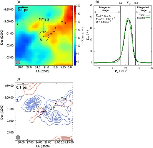
Results of our outflow search procedure for MMS 5. (a) Outflow driving source candidates overlaid on the 12CO integrated intensity map. (b) Average spectrum of the 12CO emission over the |${30^{\prime \prime }}$| radius area around the center of the left-hand panel and the result of Gaussian fitting. (c) 12CO integrated intensity maps for the distributions of blueshifted and redshifted components. In panels (a) and (c), the filled and open circles represent the same as in figure 1, and the effective angular resolution is indicated in the bottom-left. The area where the 12CO spectrum is averaged in panel (b) is indicated by the dashed circle in panel (a). In panel (b), three parameters for the fitting are indicated on the left, and the integrated velocity range for the blueshifted and redshifted components is indicated by arrows. In panel (c), the blue and red contours show the distributions of the blueshifted and redshifted components integrated from |$v_{\rm LSR} = -1.2\:$|km|$\:$|s|$^{-1}$| to |$8.2\:$|km|$\:$|s|$^{-1}$| and from |$13.8\:$|km|$\:$|s|$^{-1}$| to |$20.2\:$|km|$\:$|s|$^{-1}$|, respectively. The contour intervals are |$3\:$|K|$\:$|km|$\:$|s|$^{-1}$| (|$\sim 5\sigma )$| starting at |$3\:$|K|$\:$|km|$\:$|s|$^{-1}$|. The gray dashed line represents the axis of the outflow. In this example, we focus on the one candidate located at the center of panels (a) and (c), but we apply the same procedure independently for all other candidates. For example, the peaks located to the north and south of MMS 5 in panel (c) are regarded as outflows associated with different sources (see figures 28 and 30). (Color online)
4 Results
4.1 Identified outflows
4.1.1 Overview of identified outflows
Following the procedure described in subsection 3.2, we identified 44 CO outflows in the 12CO (|$J = 1\!-\!0$|) line, of which 17 are newly detected. To distinguish them from those detected in the |${}^{13}$|CO (|$J = 1\!-\!0$|) line, hereafter we refer to them as 12CO outflows. Figures 5 and 6 show the locations of the detected outflows and their position angles, and table 3 lists all the outflows. 25 outflows consist of a pair of blueshifted and redshifted lobes, and 19 outflows have a single lobe (13 blueshifted, and six redshifted). The integrated images and position-velocity (P–V) diagrams of the newly detected outflows are shown in figures 7–23, and those of previously known outflows are shown in the appendix. All newly detected outflows are associated with H|$_2$| jets.
Locations of the detected outflows overlaid on the 12CO (|$J = 1\!-\!0$|) total integrated intensity map which is the same as in figure 1. The red and black filled circles indicate the positions of newly detected and known outflow driving sources. Each solid line indicates the position angles of an outflow. White dashed lines represent the directions of filaments in the clouds considered in this study (see sub-subsection 4.3.3). The black squares indicate OMC 2/3, L1641-N, and NGC1999, for which close-up views are presented in figure 6. (Color online)
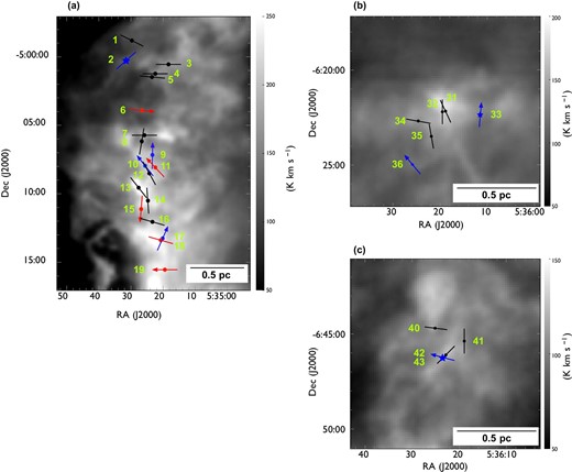
Close-up views of the detected outflows in (a) OMC 2/3, (b) L1641-N, and (c) NGC 1999. Filled circles and star symbols indicate the positions of known and newly detected outflow driving sources, respectively. Each solid line or arrow indicates the position angles of an outflow. The black, blue, and red colors represent blueshifted and redshifted pairs of, single blueshifted, and single redshifted outflows, respectively. The direction of each arrow indicates the direction of a single outflow lobe. The background grayscale image is the total integrated intensity of 12CO (|$J = 1\!-\!0$|). (Color online)
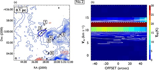
(a) Distribution of outflow No. 2, driven by a PMS star with a jet located in the northern part of OMC 3, and (b) the P–V diagram along the outflow axis. Contour levels and symbols shown in panel (a) are the same as those in figure 4d, and the thick contour represents the projected area where we estimated the mass of the outflow. In panel (a), the integrated velocity ranges of blueshifted and redshifted components are |$2.0\:$|km|$\:$|s|$^{-1}$| to |$9.5\:$|km|$\:$|s|$^{-1}$| and |$13.8\:$|km|$\:$|s|$^{-1}$| to |$20.2\:$|km|$\:$|s|$^{-1}$|, respectively. The upper (lower) limit for the blue and red ranges are indicated by the dashed lines in panel (b). The gray dashed arrow in panel (a) represents the cut along which the P–V diagram in panel (b) was obtained and also represents the position angle of the outflow. The direction of the arrow indicates the positive offset direction in the P–V diagram. The effective angular resolution of the 12CO data is shown in the lower left-hand corner. In panel (b), the contour intervals are |$1,\ 2,\ 3,\ 4$|, and |$5\:$|K in |$T_{\rm MB}$|. While the blueshifted lobe can be seen with a northwest to southeast elongation, the redshifted component is not detected. (Color online)
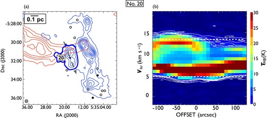
Same as in figure 7 but for outflow No. 20. In panel (a), the blueshifted and redshifted integrated intensity velocity ranges are |$-1.9\:$|km|$\:$|s|$^{-1}$| to |$4.8\:$|km|$\:$|s|$^{-1}$| and 13.1 km|$\:$|s|$^{-1}$| to |$20.2\:$|km|$\:$|s|$^{-1}$|, respectively. This outflow, located at |$\sim {10^{\prime }}$| south of the center of OMC 1, has only a blueshifted lobe and is driven by a PMS star with a jet. (Color online)
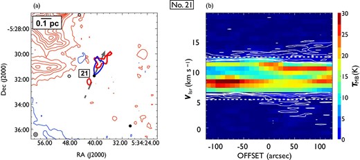
Same as in figure 7 but for outflow No. 21. In panel (a), the blueshifted and redshifted integrated intensity velocity ranges are |$-1.9\:$|km|$\:$|s|$^{-1}$| to |$4.8\:$|km|$\:$|s|$^{-1}$| and |$12.1\:$|km|$\:$|s|$^{-1}$| to |$20.2\:$|km|$\:$|s|$^{-1}$|, respectively. It can be seen that the the blueshifted lobe and redshifted lobe have a northwest elongation; the redshifted lobe also has a southeast elongation. (Color online)
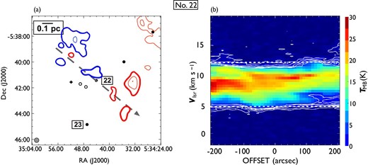
Same as in figure 7 but for outflow No. 22. In panel (a), the blueshifted and redshifted integrated intensity velocity ranges are |$-1.9\:$|km|$\:$|s|$^{-1}$| to |$4.4\:$|km|$\:$|s|$^{-1}$| and |$12.2\:$|km|$\:$|s|$^{-1}$| to |$20.2\:$|km|$\:$|s|$^{-1}$|, respectively. This bipolar outflow has multiple blueshifted and redshifted lobes with a northeast to southwest elongation. (Color online)
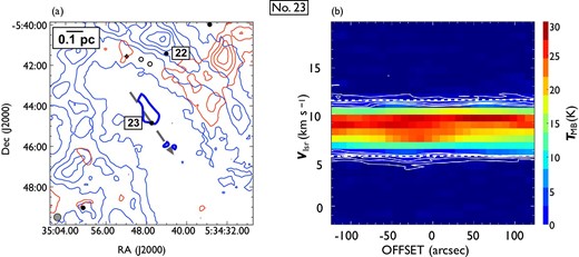
Same as in figure 7 but for outflow No. 23. In panel (a), the blueshifted and redshifted integrated intensity velocity ranges are |$-1.9\:$|km|$\:$|s|$^{-1}$| to |$5.4\:$|km|$\:$|s|$^{-1}$| and |$11.5\:$|km|$\:$|s|$^{-1}$| to |$20.2\:$|km|$\:$|s|$^{-1}$|, respectively. (Color online)
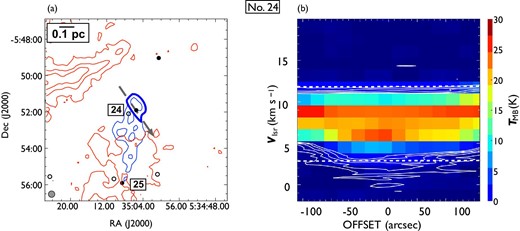
Same as in figure 7 but for outflow No. 24. In panel (a), the blueshifted and redshifted integrated intensity velocity ranges are |$-1.9\:$|km|$\:$|s|$^{-1}$| to |$3.8\:$|km|$\:$|s|$^{-1}$| and |$11.8\:$|km|$\:$|s|$^{-1}$| to |$18.0\:$|km|$\:$|s|$^{-1}$|, respectively. This blue-single outflow has a strong blueshifted lobe with a northeast to southwest elongation. The blueshifted emission south of the central source is considered to be part of outflow No. 25. (Color online)
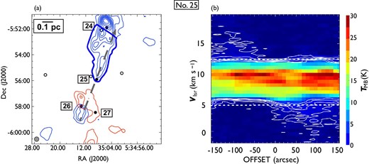
Same as in figure 7 but for outflow No. 25. In panel (a), the blueshifted and redshifted integrated intensity velocity ranges are |$-1.9\:$|km|$\:$|s|$^{-1}$| to |$4.6\:$|km|$\:$|s|$^{-1}$| and |$12.2\:$|km|$\:$|s|$^{-1}$| to |$20.2\:$|km|$\:$|s|$^{-1}$|, respectively. This single outflow has a strong blueshifted lobe in the northern direction. The redshifted emission south of the central source is considered to be part of outflow No. 27. (Color online)
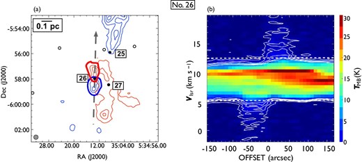
Same as in figure 7 but for outflow No. 26. In panel (a), the blueshifted and redshifted integrated intensity velocity ranges are |$-1.9\:$|km|$\:$|s|$^{-1}$| to |$4.9\:$|km|$\:$|s|$^{-1}$| and |$12.8\:$|km|$\:$|s|$^{-1}$| to |$20.2\:$|km|$\:$|s|$^{-1}$|, respectively. The blueshifted lobe in the south and redshifted lobe in the north are clearly visible. (Color online)
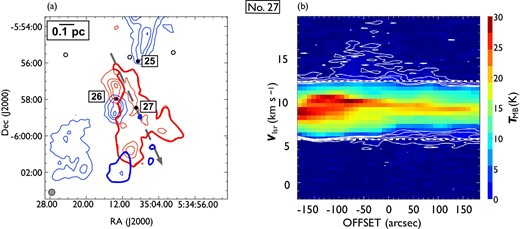
Same as in figure 7 but for outflow No. 27. In panel (a), the blueshifted and redshifted integrated intensity velocity ranges are |$-1.9\:$|km|$\:$|s|$^{-1}$| to |$5.2\:$|km|$\:$|s|$^{-1}$| and |$12.0\:$|km|$\:$|s|$^{-1}$| to |$20.2\:$|km|$\:$|s|$^{-1}$|, respectively. This outflow has strong redshifted lobes with a northeast to southwest elongation and faint blueshifted lobes with a southwest elongation. (Color online)
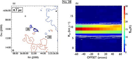
Same as in figure 7 but for outflow No. 28. In panel (a), the blueshifted and redshifted integrated intensity velocity ranges are |$-1.9\:$|km|$\:$|s|$^{-1}$| to |$5.5\:$|km|$\:$|s|$^{-1}$| and |$11.4\:$|km|$\:$|s|$^{-1}$| to |$20.2\:$|km|$\:$|s|$^{-1}$|, respectively. (Color online)
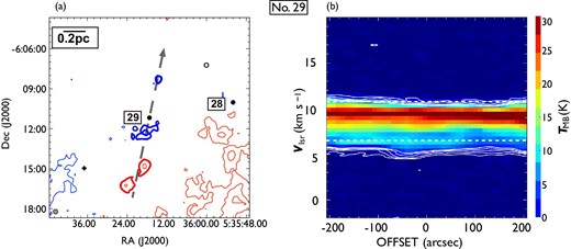
Same as figure 7, but for outflow No. 29. In panel (a), the blueshifted and redshifted integrated intensity velocity ranges are |$-1.9\:$|km|$\:$|s|$^{-1}$| to |$6.7\:$|km|$\:$|s|$^{-1}$| and |$10.9\:$|km|$\:$|s|$^{-1}$| to |$20.2\:$|km|$\:$|s|$^{-1}$|, respectively. This outflow is a faint bipolar outflow with multiple lobes in the north and south. (Color online)
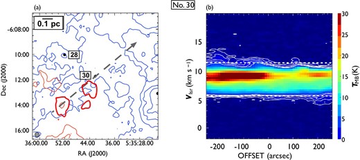
Same as figure 7, but for outflow No. 30. In panel (a), the blueshifted and redshifted integrated intensity velocity ranges are |$-1.9\:$|km|$\:$|s|$^{-1}$| to |$5.7\:$|km|$\:$|s|$^{-1}$| and |$11.5\:$|km|$\:$|s|$^{-1}$| to |$20.2\:$|km|$\:$|s|$^{-1}$|, respectively. This red-single outflow has the plural redshifted lobes with a northwest elongation. (Color online)
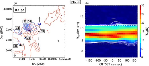
Same as in figure 7 but for outflow No. 33. In panel (a), the blueshifted and redshifted integrated intensity velocity ranges are |$-1.9\:$|km|$\:$|s|$^{-1}$| to |$3.7\:$|km|$\:$|s|$^{-1}$| and |$11.5\:$|km|$\:$|s|$^{-1}$| to |$18.0\:$|km|$\:$|s|$^{-1}$|, respectively. This faint single blue outflow is driven by the central L1641 region PMS star with a jet. (Color online)
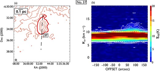
Same as in figure 7 but for outflow No. 37. In panel (a), the blueshifted and redshifted integrated intensity velocity ranges are |$-1.9\:$|km|$\:$|s|$^{-1}$| to |$6.0\:$|km|$\:$|s|$^{-1}$| and |$10.9\:$|km|$\:$|s|$^{-1}$| to |$20.2\:$|km|$\:$|s|$^{-1}$|, respectively. The redshifted lobe can clearly be seen to the north. (Color online)
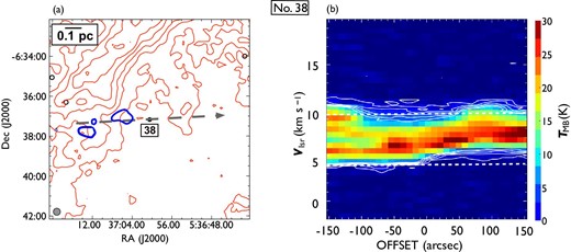
Same as in figure 7 but for outflow No. 38. In panel (a), the blueshifted and redshifted integrated intensity velocity ranges are |$-1.9\:$|km|$\:$|s|$^{-1}$| to |$3.9\:$|km|$\:$|s|$^{-1}$| and |$9.5\:$|km|$\:$|s|$^{-1}$| to |$18.0\:$|km|$\:$|s|$^{-1}$|, respectively. This faint single blue outflow has the three blueshifted components to the east. (Color online)
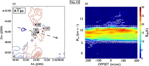
Same as in figure 7 but for outflow No. 43. In panel (a), the blueshifted and redshifted integrated intensity velocity ranges are |$-1.9\:$|km|$\:$|s|$^{-1}$| to |$4.8\:$|km|$\:$|s|$^{-1}$| and |$12.1\:$|km|$\:$|s|$^{-1}$| to |$20.2\:$|km|$\:$|s|$^{-1}$|, respectively. This single blue outflow is driven by the protostar just to the south of the HH 1/2 VLA source. (Color online)
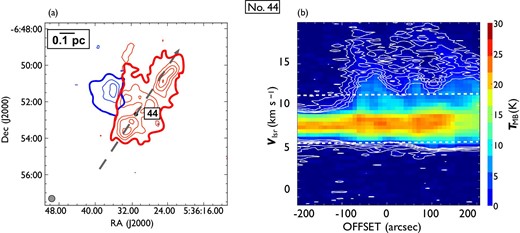
Same as in figure 7 but for outflow No. 44. In panel (a), the blueshifted and redshifted integrated intensity velocity ranges are |$-1.9\:$|km|$\:$|s|$^{-1}$| to |$5.4\:$|km|$\:$|s|$^{-1}$| and |$11.2\:$|km|$\:$|s|$^{-1}$| to |$20.2\:$|km|$\:$|s|$^{-1}$|, respectively. This outflow has a strong redshifted component with a northwest to southeast elongation and a faint blueshifted component with a northeast elongation. We define the position angle of No. 44 as the direction of the redshifted component. (Color online)
4.1.2 Detection rate of outflows
Table 4 lists the number and detection rate of outflows for the driving sources in each category. The detection rate of molecular outflows for protostars with H|$_2$| jets is 62%, which is |$\sim 15$| times higher than that for protostars without H|$_2$| jets (4%).
Outflow detection rate sorted by driving source category.
| Category | Number of outflows | Number of candidates | Detection rate |
|---|---|---|---|
| Protostar without jet | 4 | 113 | 4% |
| Protostar with jet | 33 | 53 | 62% |
| PMS star with jet | 7 | 12 | 58% |
| Total | 44 | 178 | 25% |
| Category | Number of outflows | Number of candidates | Detection rate |
|---|---|---|---|
| Protostar without jet | 4 | 113 | 4% |
| Protostar with jet | 33 | 53 | 62% |
| PMS star with jet | 7 | 12 | 58% |
| Total | 44 | 178 | 25% |
In table 4, of the 65 YSOs with H|$_2$| jets, 40 (62%) are also associated with outflows, and of the 44 YSOs associated with outflows, only four (9%) are not accompanied by H|$_2$| jets. These correlations imply that the molecular outflows and H|$_2$| jets occur in almost the same phase of star formation.
Table 5 lists the number and detection rate of outflows in each subregion. The detection rates of outflows among the subregions are consistent with each other within uncertainties, except for in OMC 1. Note that we exclude the 32 YSOs distributed in the center of OMC 1 (see section 2 and figure 1), and the detection rate of the outflows in OMC 1 is 0% to represent an incomplete sample.
Outflow detection rate in each subregion.
| Subregion | Number of outflows | Number of candidates | Detection rate* |
|---|---|---|---|
| OMC 2/3 | 19 | 62 | 31 ± 7% |
| OMC 4/5 | 11 | 59 | 19 ± 6% |
| L1641-N | 8 | 27 | 30 ± 10% |
| NGC 1999 | 6 | 19 | 32 ± 13% |
| OMC 1† | 0 | 11 | 0% |
| Subregion | Number of outflows | Number of candidates | Detection rate* |
|---|---|---|---|
| OMC 2/3 | 19 | 62 | 31 ± 7% |
| OMC 4/5 | 11 | 59 | 19 ± 6% |
| L1641-N | 8 | 27 | 30 ± 10% |
| NGC 1999 | 6 | 19 | 32 ± 13% |
| OMC 1† | 0 | 11 | 0% |
*The uncertainties |$\surd (N)$|, where N is the number of detected outflows.
†Excluding the center of OMC 1.
List of outflows.
| No. | |$\alpha$|* | |$\delta$|* | Driving source | Common name | Velocity | PA§ | New | Reference |
|---|---|---|---|---|---|---|---|---|
| (J2000.0) | (J2000.0) | category† | of driving source | shift‡ | detection | |||
| OMC 2/3 | ||||||||
| 1 | 05 35 29.72 | |$-$|04 58 48.8 | P | BR | 65 | — | 1 | |
| 2 | 05 35 31.62 | |$-$|05 00 14.0 | PMSJ | B | 130 | Yes | — | |
| 3 | 05 35 18.32 | |$-$|05 00 33.0 | PJ | MMS 2 | BR | 90 | — | 1,2,3,4 |
| 4 | 05 35 22.43 | |$-$|05 01 14.1 | PJ | MMS 5 | BR | 90 | — | 1,2,3,4 |
| 5 | 05 35 23.47 | |$-$|05 01 28.7 | PJ | MMS 6 | BR | 85 | — | 1,3 |
| 6 | 05 35 26.57 | |$-$|05 03 55.1 | PJ | MMS 7 | BR | 90 | — | 1,2,3,4 |
| 7 | 05 35 25.82 | |$-$|05 05 43.6 | PJ | MMS 9 | BR | 90 | — | 1,2,3,4 |
| 8 | 05 35 26.66 | |$-$|05 06 10.3 | P | HOPS 75 | BR | 170 | — | 1,2,3 |
| 9 | 05 35 23.33 | |$-$|05 07 09.8 | PMSJ | MMS 11 | B | 160 | — | 1,4 |
| 10 | 05 35 25.61 | |$-$|05 07 57.3 | PJ | MMS 14 | B | 40 | — | 1,2,4 |
| 11 | 05 35 22.41 | |$-$|05 08 04.8 | PMSJ | MMS 15 | R | 45 | — | 1,2,4 |
| 12 | 05 35 24.30 | |$-$|05 08 30.6 | PJ | MMS 103 | BR | 30 | — | 1,2,4 |
| 13 | 05 35 27.63 | |$-$|05 09 33.5 | PJ | FIR 3 | BR | 40 | — | 1,2,4,5 |
| 14 | 05 35 24.73 | |$-$|05 10 30.2 | PJ | VLA13 | BR | 5 | — | 1,5 |
| 15 | 05 35 26.85 | |$-$|05 11 07.3 | PMSJ | R | 175 | — | 1 | |
| 16 | 05 35 23.33 | |$-$|05 12 03.1 | PJ | FIR 6 b | BR | 75 | — | 1,6 |
| 17 | 05 35 20.14 | |$-$|05 13 15.5 | PJ | FIR 6 d | B | 155 | — | 6 |
| 18 | 05 35 20.73 | |$-$|05 13 23.6 | P | FIR 6 c | R | 75 | — | 1,6 |
| 19 | 05 35 19.47 | |$-$|05 15 32.7 | P | CSO 33 | R | 90 | — | 1 |
| OMC 4/5 | ||||||||
| 20 | 05 35 18.28 | |$-$|05 31 42.1 | PMSJ | B | 15 | Yes | — | |
| 21 | 05 34 40.91 | |$-$|05 31 44.4 | PJ | BR | 145 | Yes | — | |
| 22 | 05 34 44.06 | |$-$|05 41 25.9 | PJ | BR | 40 | Yes | — | |
| 23 | 05 34 46.94 | |$-$|05 44 50.9 | PJ | B | 30 | Yes | — | |
| 24 | 05 35 05.49 | |$-$|05 51 54.4 | PJ | B | 30 | Yes | — | |
| 25 | 05 35 08.60 | |$-$|05 55 54.3 | PJ | B | 160 | Yes | — | |
| 26 | 05 35 13.41 | |$-$|05 57 58.1 | PJ | Ori 2-6 | BR | 0 | Yes | — |
| 27 | 05 35 09.00 | |$-$|05 58 27.6 | PJ | BR | 25 | Yes | — | |
| 28 | 05 35 52.00 | |$-$|06 10 01.8 | PJ | B | 60 | Yes | — | |
| 29 | 05 36 17.26 | |$-$|06 11 11.0 | PJ | BR | 165 | Yes | — | |
| 30 | 05 35 42.18 | |$-$|06 11 43.8 | PMSJ | R | 135 | Yes | — | |
| L1641-N | ||||||||
| 31 | 05 36 18.83 | |$-$|06 22 10.2 | PJ | BR | 25 | — | 7,8 | |
| 32 | 05 36 19.50 | |$-$|06 22 12.3 | PJ | BR | 0 | — | 7,8 | |
| 33 | 05 36 11.45 | |$-$|06 22 22.1 | PMSJ | B | 175 | Yes | 7,8 | |
| 34 | 05 36 24.61 | |$-$|06 22 41.3 | PJ | BR | 80 | — | 7,8 | |
| 35 | 05 36 21.84 | |$-$|06 23 29.8 | PJ | BR | 10 | — | 7,8 | |
| 36 | 05 36 25.86 | |$-$|06 24 58.7 | PJ | B | 40 | — | 7,8 | |
| 37 | 05 35 50.02 | |$-$|06 34 53.4 | PJ | R | 175 | Yes | — | |
| 38 | 05 37 00.45 | |$-$|06 37 10.5 | P | B | 95 | Yes | — | |
| NGC 1999 | ||||||||
| 39 | 05 36 36.10 | |$-$|06 38 52.0 | PJ | V380 Ori-NE | BR | 0 | — | 9,10 |
| 40 | 05 36 25.13 | |$-$|06 44 41.8 | PJ | IRS 63 (HH 147) | BR | 80 | — | 11 |
| 41 | 05 36 18.93 | |$-$|06 45 22.7 | PJ | VLA 3, HOPS 168 | BR | 0 | — | 11 |
| 42 | 05 36 22.84 | |$-$|06 46 06.2 | PJ | VLA 1/2 (HH 1/2) | BR | 140 | — | 11 |
| 43 | 05 36 23.54 | |$-$|06 46 14.5 | PJ | IRS 121 (HH36) | B | 75 | Yes | 11 |
| 44 | 05 36 30.97 | |$-$|06 52 40.9 | PJ | BR | 150 | Yes | — | |
*Coordinates of the outflow driving source.
†Category of the outflow driving sources. “P”, “PJ”, and “PMSJ” represent protostars without H|$_2$| jet, protostars with H|$_2$| jet and PMS stars with H|$_2$| jet, respectively.
‡The velocity shifts of outflows. “BR”, “B”, and “R” represent blue and redshifted pairs of, single blueshifted, and single redshifted outflows, respectively.
§Outflow position angle on the plane of the sky (|$5^{\circ }$| bin). References—1, Takahashi et al. (2008); 2, Williams et al. (2003); 3, Aso et al. (2000); 4, Chini et al. 1997; 5, Shimaziri et al. (2008); 6, Shimajiri et al. (2009); 7, Nakamura et al. (2012); 8, Stanke and Williams (2007); 9, Davis et al. (2000); 10, Choi et al. (2017); 11, Moro-Martín et al. (1999).
4.2 Optical depth of 12CO outflows
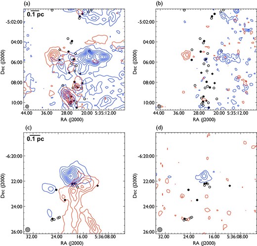
Pair of 12CO and |${}^{13}$|CO outflows. Panels (a) and (c) show 12CO outflows following the procedure described in subsection 3.2. Contours and markers are the same as those in figure 4d. Panels (b) and (d) show |${}^{13}$|CO outflows with the same velocity ranges as panels (a) and (c), respectively. The contour increments are |$0.3\:$|K|$\:$|km|$\:$|s|$^{-1}$| (|$\sim 1 \sigma$|) starting at |$0.9\:$|K|$\:$|km|$\:$|s|$^{-1}$| (|$\sim 3 \sigma$|). (Color online)
Optical depth of outflows.
| No. | Lobe | |$\tau _{{}^{13}\rm CO}$| | |$\tau _{{}^{12}\rm CO}$| |
|---|---|---|---|
| 7 | Blue | 0.075 | 4.65 |
| 7 | Red | 0.097 | 6.01 |
| 31–32 | Blue | 0.076 | 4.71 |
| No. | Lobe | |$\tau _{{}^{13}\rm CO}$| | |$\tau _{{}^{12}\rm CO}$| |
|---|---|---|---|
| 7 | Blue | 0.075 | 4.65 |
| 7 | Red | 0.097 | 6.01 |
| 31–32 | Blue | 0.076 | 4.71 |
4.3 Outflow and cloud properties
4.3.1 Physical parameters of outflows
To estimate the physical parameters of each detected outflow, we assume that the |$\rm {}^{12}CO$| molecules are in LTE. The results are summarized in table 7, but we do not correct for the inclination angle of outflows. When the outflows are distributed randomly, the average of inclinations is |$57.^{\!\!\!\circ }3$|, and the velocity of outflows will be increased by a factor of 1.85, while the timescale of outflows will be decreased by a factor of 0.64. The uncertainty arising from unknown inclination angles of outflows is large. For example, in the rather extreme case of |$80^{\circ }$|, the velocity will be higher by a factor of 5.76.
|$\rm {}^{12}CO$|(1–0) outflow properties.
| No. | Lobe | |$M_{\rm flow}$|* | |$P_{\rm flow}$| | |$E_{\rm flow}$| | |$\Delta v_{\rm max}$| | |$R_{\rm max}$| | |$t_{\rm d}$| | |$\dot{M}_{\rm flow}$| | |$\dot{P}_{\rm flow}$| | |$\dot{E}_{\rm flow}$| |
|---|---|---|---|---|---|---|---|---|---|---|
| |$(M_{\odot })$| | |$(M_{\odot }\:\mbox{km}\:\mbox{s}^{-1})$| | |$(10^{43}\:\mbox{erg})$| | (km|$\:$|s|$^{-1}$|) | (pc) | (|$10^4\:$|yr) | (|$10^{-6}\, M_{\odot }\:$|yr|$^{-1}$|) | |$(10^{-6}M_{\odot }\:\mbox{km}\:\mbox{s}^{-1}\:\mbox{yr}^{-1})$| | |$(10^{30}\:\mbox{erg}\:\mbox{s}^{-1})$| | ||
| OMC 2/3 | ||||||||||
| 1 | B | 0.07 ± 0.03 | 0.26 ± 0.11 | 1.00 ± 0.45 | 5.3 | 0.13 | 2.4 | 3.0 | 10.6 | 13.1 |
| R | 0.11 ± 0.04 | 0.24 ± 0.10 | 0.63 ± 0.27 | 3.9 | 0.23 | 5.9 | 1.5 | 4.0 | 3.5 | |
| 2 | B | 0.16 ± 0.07 | 0.61 ± 0.27 | 2.40 ± 1.15 | 6.6 | 0.08 | 1.2 | 14.1 | 50.3 | 65.9 |
| 3 | B | 0.03 ± 0.02 | 0.13 ± 0.09 | 0.64 ± 0.45 | 6.4 | 0.06 | 0.9 | 2.5 | 14.1 | 21.1 |
| R | 0.16 ± 0.06 | 0.55 ± 0.21 | 1.96 ± 0.79 | 6.2 | 0.19 | 3.0 | 5.0 | 18.6 | 20.6 | |
| 4 | B | 0.20 ± 0.07 | 0.96 ± 0.37 | 4.87 ± 1.72 | 6.7 | 0.08 | 1.1 | 17.6 | 87.0 | 136.8 |
| R | 0.07 ± 0.03 | 0.23 ± 0.11 | 0.79 ± 0.29 | 5.9 | 0.06 | 1.0 | 6.0 | 22.6 | 24.6 | |
| 5 | B | 0.37 ± 0.14 | 1.92 ± 0.79 | 10.54 ± 4.04 | 10.3 | 0.32 | 3.1 | 12.1 | 61.9 | 108.6 |
| R | 0.01 ± 0.01 | 0.02 ± 0.01 | 0.06 ± 0.05 | 3.7 | 0.05 | 1.2 | 0.5 | 1.5 | 1.5 | |
| 6 | B | 0.01 ± 0.01 | 0.02 ± 0.01 | 0.04 ± 0.02 | 3.5 | 0.08 | 2.2 | 0.4 | 0.9 | 0.6 |
| R | 1.04 ± 0.23 | 4.34 ± 1.04 | 18.23 ± 4.78 | 7.4 | 0.55 | 7.3 | 14.6 | 59.4 | 79.5 | |
| 7 | B | 2.29 ± 0.36 | 10.60 ± 2.09 | 53.39 ± 11.54 | 13.0 | 0.42 | 3.1 | 73.2 | 341.8 | 539.4 |
| R(west) | 1.55 ± 0.30 | 5.80 ± 1.63 | 22.70 ± 5.85 | 8.4 | 0.34 | 4.0 | 39.2 | 145.2 | 181.4 | |
| R(east) | 0.13 ± 0.04 | 0.46 ± 0.15 | 1.61 ± 0.52 | 4.0 | 0.27 | 6.1 | 1.5 | 7.5 | 5.0 | |
| 8 | B | 0.14 ± 0.05 | 0.72 ± 0.28 | 3.76 ± 1.60 | 7.9 | 0.13 | 1.6 | 9.1 | 45.3 | 73.9 |
| R | 0.20 ± 0.05 | 0.74 ± 0.18 | 2.83 ± 0.73 | 4.7 | 0.13 | 2.7 | 7.0 | 27.7 | 32.7 | |
| 9 | B | 0.14 ± 0.04 | 0.69 ± 0.22 | 3.51 ± 1.17 | 6.8 | 0.1 | 1.4 | 9.6 | 49.3 | 77.5 |
| 10 | B | 0.63 ± 0.16 | 2.68 ± 0.71 | 11.36 ± 3.30 | 6.9 | 0.34 | 4.8 | 13.1 | 55.8 | 73.9 |
| 11 | R | 0.18 ± 0.04 | 0.66 ± 0.17 | 2.51 ± 0.55 | 5.2 | 0.09 | 1.7 | 10.1 | 38.7 | 46.3 |
| 12 | B | 0.10 ± 0.05 | 0.46 ± 0.24 | 2.13 ± 1.16 | 6.3 | 0.06 | 0.9 | 10.6 | 51.3 | 72.9 |
| R | 0.31 ± 0.10 | 1.30 ± 0.44 | 5.76 ± 1.99 | 7.7 | 0.08 | 1.0 | 30.2 | 130.3 | 178.6 | |
| 13 | B(north) | 0.40 ± 0.15 | 2.29 ± 0.97 | 14.32 ± 6.81 | 12.7 | 0.14 | 1.1 | 36.7 | 208.2 | 419.5 |
| B(south) | 0.30 ± 0.10 | 1.54 ± 0.54 | 8.20 ± 3.19 | 8.5 | 0.12 | 1.4 | 21.6 | 110.2 | 187.6 | |
| R(north) | 0.36 ± 0.11 | 1.69 ± 0.57 | 8.30 ± 3.17 | 9.1 | 0.13 | 1.4 | 26.2 | 120.7 | 188.6 | |
| R(south) | 0.32 ± 0.10 | 1.48 ± 0.50 | 7.07 ± 2.70 | 9.1 | 0.10 | 1.1 | 30.2 | 134.3 | 208.7 | |
| 14 | B(south) | 0.09 ± 0.03 | 0.39 ± 0.14 | 1.76 ± 0.69 | 5.8 | 0.08 | 1.4 | 6.5 | 28.2 | 40.7 |
| R(south) | 0.13 ± 0.05 | 0.59 ± 0.24 | 2.73 ± 1.19 | 6.3 | 0.10 | 1.6 | 8.6 | 36.7 | 54.8 | |
| 15 | R | 0.16 ± 0.06 | 0.64 ± 0.26 | 2.57 ± 1.10 | 5.0 | 0.26 | 5.1 | 3.0 | 12.6 | 16.1 |
| 16 | B | 0.38 ± 0.12 | 1.70 ± 0.56 | 7.60 ± 2.80 | 6.9 | 0.22 | 3.1 | 12.1 | 54.8 | 76.5 |
| R | 0.22 ± 0.08 | 0.87 ± 0.35 | 3.70 ± 1.48 | 7.0 | 0.24 | 3.4 | 6.0 | 25.7 | 34.7 | |
| 17 | B | 0.49 ± 0.19 | 2.36 ± 0.98 | 11.78 ± 5.01 | 8.3 | 0.54 | 6.3 | 7.5 | 37.2 | 58.9 |
| 18 | R | 0.27 ± 0.12 | 1.25 ± 0.55 | 5.83 ± 2.72 | 6.7 | 0.12 | 1.8 | 15.1 | 69.4 | 105.6 |
| 19 | R | 0.36 ± 0.13 | 1.80 ± 0.68 | 8.93 ± 3.55 | 6.8 | 0.16 | 2.3 | 15.6 | 78.0 | 122.2 |
| OMC 4/5 | ||||||||||
| 20 | B | 0.06 ± 0.02 | 0.32 ± 0.09 | 1.64 ± 0.47 | 5.7 | 0.12 | 2.1 | 3.0 | 15.1 | 24.6 |
| 21 | B | 0.04 ± 0.02 | 0.12 ± 0.08 | 0.44 ± 0.30 | 5.6 | 0.15 | 2.7 | 1.3 | 4.5 | 5.1 |
| R | 0.05 ± 0.03 | 0.29 ± 0.17 | 1.93 ± 1.16 | 7.6 | 0.17 | 2.2 | 2.0 | 13.3 | 28.1 | |
| 22 | B | 0.07 ± 0.03 | 0.30 ± 0.12 | 1.30 ± 0.50 | 5.0 | 0.28 | 5.5 | 1.2 | 5.4 | 7.5 |
| R | 0.04 ± 0.03 | 0.22 ± 0.15 | 1.22 ± 0.34 | 7.0 | 0.51 | 7.1 | 0.5 | 3.0 | 5.4 | |
| 23 | B | 0.09 ± 0.03 | 0.29 ± 0.11 | 0.99 ± 0.38 | 4.0 | 0.18 | 4.5 | 1.9 | 6.5 | 7.0 |
| 24 | B | 0.18 ± 0.09 | 1.29 ± 0.67 | 9.47 ± 5.17 | 11.7 | 0.25 | 2.1 | 8.6 | 61.9 | 144.9 |
| 25 | B | 0.24 ± 0.11 | 1.27 ± 0.61 | 7.02 ± 2.23 | 10.1 | 0.28 | 2.7 | 9.0 | 47.3 | 83.0 |
| 26 | B | 0.13 ± 0.07 | 0.70 ± 0.38 | 4.06 ± 1.68 | 10.7 | 0.14 | 1.3 | 9.8 | 53.2 | 97.4 |
| R | 0.22 ± 0.11 | 1.25 ± 0.67 | 8.60 ± 5.05 | 12.3 | 0.15 | 1.2 | 18.3 | 102.4 | 223.0 | |
| 27 | B | 0.07 ± 0.04 | 0.26 ± 0.16 | 1.07 ± 0.63 | 4.6 | 0.25 | 5.3 | 1.2 | 5.0 | 6.4 |
| R | 0.45 ± 0.26 | 2.33 ± 1.41 | 12.83 ± 4.77 | 12.4 | 0.35 | 2.7 | 16.6 | 85.2 | 148.9 | |
| 28 | B | 0.05 ± 0.03 | 0.18 ± 0.11 | 0.62 ± 0.38 | 4.1 | 0.16 | 3.8 | 1.3 | 4.6 | 5.2 |
| 29 | B | 0.08 ± 0.04 | 0.32 ± 0.18 | 1.33 ± 0.73 | 4.7 | 0.38 | 7.9 | 1.0 | 4.1 | 5.3 |
| R | 0.05 ± 0.02 | 0.16 ± 0.07 | 0.49 ± 0.22 | 3.7 | 0.40 | 10.7 | 0.5 | 1.5 | 1.4 | |
| 30 | R | 0.22 ± 0.10 | 0.80 ± 0.37 | 2.99 ± 1.47 | 5.6 | 0.30 | 5.3 | 4.1 | 15.1 | 18.0 |
| L1641-N | ||||||||||
| 31 | B(northwest) | 0.36 ± 0.09 | 2.09 ± 0.65 | 13.66 ± 5.06 | 19.8 | 0.17 | 0.8 | 43.3 | 261.4 | 528.5 |
| R(southeast) | 0.14 ± 0.08 | 0.77 ± 0.46 | 4.48 ± 2.72 | 8.2 | 0.65 | 7.8 | 2.0 | 10.1 | 18.1 | |
| B(east) | 0.05 ± 0.02 | 0.24 ± 0.07 | 1.19 ± 0.35 | 5.4 | 0.16 | 2.8 | 1.5 | 8.6 | 13.1 | |
| 32 | B(north) | 0.36 ± 0.08 | 1.94 ± 0.49 | 10.92 ± 3.19 | 11.0 | 0.19 | 1.7 | 21.4 | 114.5 | 203.4 |
| R(south) | 0.48 ± 0.28 | 2.73 ± 1.66 | 16.07 ± 10.19 | 15.4 | 1.01 | 6.3 | 7.5 | 42.8 | 79.5 | |
| 33 | B | 0.02 ± 0.01 | 0.07 ± 0.04 | 0.29 ± 0.15 | 4.7 | 0.15 | 3.1 | 0.5 | 2.5 | 3.0 |
| 34 | B | 0.04 ± 0.02 | 0.16 ± 0.08 | 0.74 ± 0.30 | 5.6 | 0.15 | 2.6 | 1.3 | 6.0 | 9.0 |
| R | 0.03 ± 0.01 | 0.12 ± 0.04 | 0.55 ± 0.07 | 5.8 | 0.08 | 1.3 | 1.8 | 9.0 | 14.0 | |
| 35 | B | 0.01 ± 0.01 | 0.03 ± 0.02 | 0.13 ± 0.08 | 4.7 | 0.04 | 0.8 | 0.9 | 3.6 | 4.9 |
| R | 0.02 ± 0.01 | 0.12 ± 0.07 | 0.72 ± 0.34 | 9.9 | 0.06 | 0.5 | 4.0 | 22.0 | 41.7 | |
| 36 | B | 0.01 ± 0.01 | 0.04 ± 0.03 | 0.19 ± 0.12 | 5.0 | 0.08 | 1.6 | 0.6 | 2.6 | 3.7 |
| 37 | R | 0.42 ± 0.08 | 1.00 ± 0.23 | 2.60 ± 0.73 | 4.9 | 0.25 | 5.1 | 8.2 | 19.6 | 16.1 |
| 38 | B | 0.04 ± 0.02 | 0.11 ± 0.05 | 0.33 ± 0.14 | 3.6 | 0.22 | 5.8 | 0.6 | 1.9 | 1.8 |
| NGC 1999 | ||||||||||
| 39 | B | 0.32 ± 0.13 | 1.63 ± 0.81 | 9.62 ± 4.13 | 11.6 | 0.23 | 1.9 | 16.0 | 85.5 | 157.5 |
| R | 0.16 ± 0.09 | 0.85 ± 0.49 | 4.94 ± 2.24 | 9.3 | 0.22 | 2.3 | 7.0 | 36.5 | 68.0 | |
| 40 | B | 0.02 ± 0.01 | 0.07 ± 0.05 | 6.38 ± 0.17 | 4.9 | 0.06 | 1.2 | 1.5 | 5.5 | 6.5 |
| R | 0.27 ± 0.12 | 1.34 ± 0.61 | 6.83 ± 1.71 | 8.3 | 0.14 | 1.6 | 11.5 | 83.0 | 132.0 | |
| 41 | B | 0.01 ± 0.01 | 0.04 ± 0.03 | 0.11 ± 0.08 | 3.0 | 0.06 | 2.0 | 0.5 | 2.0 | 2.0 |
| R | 0.08 ± 0.05 | 0.44 ± 0.27 | 2.53 ± 1.65 | 8.8 | 0.22 | 2.5 | 3.5 | 17.5 | 32.0 | |
| 42 | B | 0.07 ± 0.03 | 0.27 ± 0.13 | 1.15 ± 0.55 | 4.2 | 0.46 | 10.7 | 0.5 | 2.5 | 3.5 |
| R | 0.10 ± 0.06 | 0.44 ± 0.29 | 2.09 ± 0.39 | 6.6 | 0.46 | 6.9 | 1.5 | 6.5 | 9.5 | |
| 43 | B | 0.04 ± 0.02 | 0.16 ± 0.10 | 0.73 ± 0.47 | 6.0 | 0.37 | 6.0 | 0.5 | 2.5 | 4.0 |
| 44 | B | 0.07 ± 0.04 | 0.30 ± 0.14 | 1.26 ± 0.58 | 4.7 | 0.34 | 7.1 | 1.0 | 4.0 | 5.5 |
| R | 1.42 ± 0.53 | 9.13 ± 3.77 | 63.03 ± 20.54 | 13.3 | 0.46 | 3.4 | 41.5 | 267.0 | 585.0 | |
| Total | 21.5 | 84.2 | 439.7 | 728.9 | 3585.0 | 6024.8 | ||||
* The error is estimated by applying noise of |$\pm 3\sigma$| to pixels with emission above 3|$\sigma$|.
Figure 25 shows histograms of the mass, momentum, energy, mass outflow rate, momentum ejection rate, and energy ejection rate for all outflows and a histogram of dynamical timescale for all outflow lobes. The average values of mass, momentum, energy, mass outflow rate, momentum ejection rate, and energy ejection rate of all outflows in our sample are |$4.8\times 10^{-1}\, M_{\odot }$|, |$1.9\, M_{\odot }\:$|km|$\:$|s|$^{-1}$|, |$1.0\times 10^{44}\:$|erg, |$1.7 \times 10^{-5}\, M_{\odot }\:$|yr|$^{-1}$|, |$8.1\times 10^{-5}\, M_{\odot }\:$|km|$\:$|s|$^{-1}\:$|yr|$^{-1}$|, and |$1.4\times 10^{32}\:$|erg|$\:$|s|$^{-1}$|, respectively. The average dynamical timescale of all outflow lobes is |$3.8\times 10^4\:$|yr.
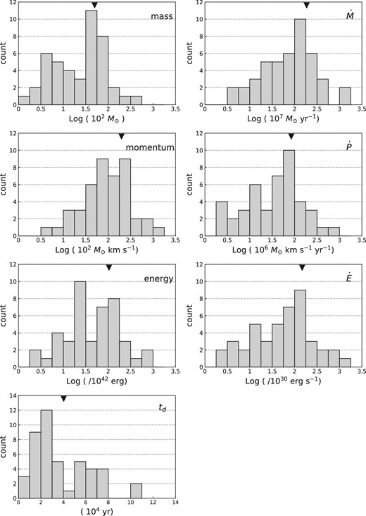
Histograms of various outflow properties. Each triangle represents the average of the corresponding property.
4.3.2 Properties of clouds
Cloud parameters of Orion A.
| Subregion | |$M_{\rm cl}$| | |${}^{13}\rm CO\ \sigma _{v}$| | |$\mathcal {E}_{\rm turb}$| |
|---|---|---|---|
| (|$10^{3}\, M_{\odot }$|) | (km|$\:$|s|$^{-1}$|) | (10|$^{46}$| erg) | |
| OMC 2/3 | 5.8 | 0.9 | 13.0 |
| OMC 4/5 | 9.6 | 1.3 | 31.2 |
| L1641-N | 5.0 | 1.5 | 21.0 |
| NGC 1999 | 4.5 | 1.2 | 13.6 |
| OMC 1 | 7.1 | 1.7 | 28.2 |
| Total | 32.0 | 107.0 |
4.3.3 Position angle of outflows
Prototars formed in filamentary structures may have a characteristic outflow direction relative to a filament: parallel or perpendicular (Stephens et al. 2017). According to Stephens et al. (2017), the projected angles between the outflows and filaments in the Perseus molecular cloud complex are not consistent with being either mostly parallel or perpendicular; they are consistent with being random or a mix of parallel and perpendicular. While Kong et al. (2019) conclude that outflows in the Dark cloud |${\rm G}28.37 + 0.07$| are perpendicular to their parent filament. We also compare the position angles of the outflows to the direction of the cloud filament in Orion A. For simplification, we define the direction of the cloud filament on the plane of the sky as PA |$=\ -20^{\circ }$| for |$\delta$||$\ge -5^{\circ }$||${05^{\prime }00^{^{\prime\prime}_{.}}00}$| (J2000.0), PA |$=\ 10^{\circ }$| for |$-5^{\circ }$||${05^{\prime }00^{^{\prime\prime}_{.}}00}$| (J2000.0) |$\gt $||$\delta$||$\ge -5^{\circ }$||${40^{\prime }00^{^{\prime\prime}_{.}}00}$| (J2000.0) and PA |$=\ -20^{\circ }$| for |$\delta$||$\le -5^{\circ }$||${40^{\prime }00^{^{\prime\prime}_{.}}00}$| (J2000.0) (see figure 5), and we determine the relative position angles of the outflows with respect to the cloud filament. The results are shown in figure 26. There is no clear significant difference between the north and the south of the clouds, and the results do not show any correlation between the position angles of the outflows and elongations of the cloud filaments.
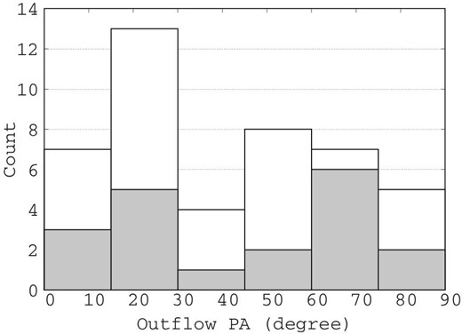
Distribution of the observed angle between outflow position angle and the cloud filament (|$15^\circ$| bins) for all outflows in Orion A (white filled) and for northern OMC 2/3 outflows (gray filled).
4.4 Comparison with previous outflow searches
In this section, we compare our results of outflow search results with those of previous surveys.
4.4.1 OMC 2/3
In OMC 2/3, 12CO (|$J = 1\!-\!0$|) outflow surveys were conducted by several authors: Aso et al. (2000) with the Nobeyama 45 m telescope, Williams et al. (2003) with the FCRAO 14 m telescope and the Berkeley–Illinois–Maryland Association (BIMA) array, and Shimajiri et al. (2008, 2009) with the Nobeyama Millimeter Array (NMA) in the OMC 2 FIR 3, 4, 5, and 6 regions. 12CO (|$J = 2\!-\!1$|) outflow surveys were conducted by Chini et al. (1997) with the National Radio Astronomy Observatory (NRAO) 12 m telescope and Takahashi et al. (2008) with the Atacama Submillimeter Telescope Experiment (ASTE). Takahashi et al. (2008) also observed the 12CO (|$J = 3\!-\!2$|) line.
All outflows detected by Chini et al. (1997), Aso et al. (2000), and Williams et al. (2003) are also detected in this study, except for an outflow associated with MMS 8. The outflow from MMS 8 was detected by Williams et al. (2003) as a bipolar outflow, while our map only reveals a blue lobe located around MMS 8. We find a counter red lobe that is at the opposite side of the HOPS 75 protostar located at |$\sim {1^{\prime }}$| south of MMS 8. We therefore identify these blueshifted and redshifted lobes as a bipolar outflow associated with HOPS 75 (our No. 8). Two independent H|$_2$| jets associated with MMS 11 and MMS 15 were detected by Davis et al. (2009), and we identify two single-lobe outflows associated with MMS 11 (redshifted lobe) and MMS 15 (blueshifted lobe). These blueshifted and redshifted lobes were identified as a bipolar outflow associated with FIR 1 by Williams et al. (2003) and Takahashi et al. (2008). We detect a redshifted single outflow associated with FIR 6c (No. 18). This outflow was clearly identified as bipolar outflows associated with FIR 6c by Takahashi et al. (2008) and Shimajiri et al. (2009). We detect 12 out of 14 outflows detected by Takahashi et al. (2008). In the two outflows not detected by this study, the velocity range detected as an outflow in the (3–2) line is buried in ambient clouds in the (1–0) line. We detect a blueshifted lobe located at |$\sim {4^{\prime }}$| northwest of FIR 6d (No. 17), but Shimajiri et al. (2009) detected bipolar outflows associated with FIR 6d. The sizes of the blueshifted lobes associated with FIR 6d detected in this study and by Shimajiri et al. (2009) are different. Outflow No. 2, which is a blueshifted single-lobe outflow, was not detected in the previous searches.
While the outflow mass obtained in subsection 4.3, which is considered the correction for optical depth, is in good agreement with that found by Takahashi et al. (2008), the momentum of the outflows of No. 13 obtained in our study is one order of magnitude higher than that found by Takahashi et al. (2008). The total mass and momentum of outflows in OMC 2/3 in our study are 107% and 29% of those determined by Takahashi et al. (2008), respectively. These discrepancies are mainly from the differences in our estimation method. Our estimations of mass and momentum of the outflows are based on the channel maps (details described in subsection 4.3), while Takahashi et al. (2008) estimated the momentum of outflows by simply multiplying the total mass with the maximum velocity of outflows. Thus, the momenta obtained by Takahashi et al. (2008) should be regarded as upper limits.
4.4.2 OMC 4/5
In OMC 4/5, no systematic search of outflows had been conducted previously. Thus, all 11 outflows identified in this region are new detections.
4.4.3 L1641-N
Our results in the central region of L1641-N agree with the previous 12CO (|$J = 2\!-\!1$|) and 12CO (|$J = 1\!-\!0$|) observations conducted by Stanke and Williams (2007) and Nakamura et al. (2012). In addition, we find three new outflows in this region. Outflow No. 33 is a blueshifted single-lobe outflow associated with IRS 50, categorized as a PMS star with H|$_2$| jets located in the central region of L1641-N. No. 37 and No. 38 are single-lobe outflows located |$\sim {15^{\prime }}$| south of the central region of L1641-N.
4.4.4 NGC 1999
In the NGC 1999 region, we detect a well-collimated CO outflow associated with V380 Ori-NE, which had already been identified by previous searches [e.g., Davis et al. 2000:12CO (|$J = 3\!-\!2$|) and (|$J = 4\!-\!3$|); and Choi et al. 2017: SiO (|$v=0$|, |$J=1\!-\!0$|)]. Our results for the outflow surveys around HH 1/2 in NGC 1999 agree with the 12CO (|$J = 1\!-\!0$|) and (|$J = 2\!-\!1$|) surveys conducted by Moro-Martín et al. (1999). This study reveals that a faint blueshifted emission located |$\sim {2^{\prime }}$| east of HH 1/2 is an outflow driven by IRS 121 (No. 43). In addition, we find a new outflow (No. 44) in this region.
The masses of the outflows associated with V380 Ori-NE and HH 1/2 are consistent with those determined by Davis et al. (2000) and Moro-Martín et al. (1999), respectively.
5 Discussion
5.1 Feedback of outflows in Orion A
With our sample of the outflows of Orion A, we estimate the dynamical effect of the outflows on the molecular clouds. Table 9 compares the kinetic energy of the cloud turbulence to the energy ejected by the outflows in each subregion. It should be noted that in table 9, each outflow parameter is corrected for the inclination angle to be |$57.^{\!\!\!\circ }3$|, which is the average value for the case of random inclination angles (see sub-subsection 4.3.1). The total energy of the outflows is only |$\sim 1.9$|% of the turbulent energy of the cloud, excluding OMC 1. This is similar to the Taurus outflows reported by Li et al. (2015). In the Taurus molecular cloud, the energy of all outflows detected by Li et al. (2015) is |$\sim 1.2$|% of the turbulent energy of the cloud.
Energy, momentum, and ejection rate of outflows and cloud turbulence.
| Subregion | |$\mathcal {E}_{\rm turb}$| | |$\mathcal {E_{\rm flow}}$|* | |$\mathcal {P}_{\rm turb}$| | |$\mathcal {P_{\rm flow}}$|* | |$\dot{\mathcal {E}}_{\rm turb}$| | |$\dot{\mathcal {E}_{\rm flow}}$|* | |$\dot{\mathcal {E}}_{\rm shell}$| † | |$\dot{\mathcal {P}}_{\rm turb}$| | |$\dot{\mathcal {P}_{\rm flow}}$|* | |$\dot{\mathcal {P}}_{\rm shell}$| † |
|---|---|---|---|---|---|---|---|---|---|---|
| (|$10^{46}\:$|erg) | (|$10^{3}\, M_{\odot }\:$|km|$\:$|s|$^{-1}$|) | (10|$^{33}\:$|erg|$\:$|s|$^{-1}$|) | (|$10^{-3}\, M_{\odot }\:$|km|$\:$|s|$^{-1}\:$|yr|$^{-1}$|) | |||||||
| OMC 2/3 | 13.0 | 0.80 | 8.7 | 0.093 | 1.9 | 17.4 | 4.0 | 4.7 | 6.1 | 6.0 |
| OMC 4/5 | 31.2 | 0.19 | 17.4 | 0.019 | 5.5 | 4.3 | 26.8 | 11.6 | 1.2 | 22.1 |
| L1641-N | 21.0 | 0.18 | 10.3 | 0.017 | 4.2 | 5.0 | 3.5 | 7.7 | 1.4 | 4.5 |
| NGC 1999 | 13.6 | 0.34 | 7.8 | 0.027 | 2.0 | 5.3 | 2.6 | 4.3 | 1.5 | 3.7 |
| Subtotal | 78.8 | 1.51 | 44.2 | 0.156 | 13.6 | 32.0 | 36.9 | 28.3 | 10.2 | 36.3 |
| OMC 1 | 28.2 | 15‡ | 14.2 | 6.4 | 4000‡ | 7.2 | 12.2 | 566‡ | 8.6 | |
*Corrected for the inclination angle.
†Feddersen et al. (2018).
‡These values are from Snell et al. (1984) 12CO (|$J = 1\!-\!0$|), Kwan and Scoville (1976) 12CO (|$J = 1\!-\!0$|), and Zapata et al. (2005) 12CO (|$J = 2\!-\!1$|). In OMC 1, the massive velocity outflows (|$\sim 100\:$|km|$\:$|s|$^{-1}$|) in Orion KL account for a large fraction of their energy and momentum. The outflows in OMC 1 have sufficient energy and momentum to maintain cloud turbulence in OMC 1.
We also compare the momentum of the outflows with that of the cloud turbulence, |$\mathcal {P}_{\rm turb}=(2M_{\rm cl}\mathcal {E}_{\rm turb})^{1/2}$|, and the results are listed in table 9. The total momentum of the outflows is |$\sim 0.4$|% of the cloud turbulence.
Besides molecular outflows, molecular shells may be another driver of turbulence in parent molecular clouds (Churchwell et al. 2006). Molecular shells show expanding spherical structures of molecular gas and are driven by protostars or intermediate-mass stars (e.g., see Arce at al. 2011; Offner & Arce 2015). In Orion A, Feddersen et al. (2018) identified molecular shells (see figure 2) and estimated that the total energy and momentum ejection rate of the shells, excluding OMC 1, were |$36.7\times 10^{33}\:$|erg|$\:$|s|$^{-1}$| and |$36.3\times 10^{-3}\, M_{\odot }\:$|km|$\:$|s|$^{-1}\:$|yr|$^{-1}$|, respectively. Those results are comparable with the energy and momentum ejection rate of the outflows.
Note that the Orion cloud complex is assumed to be located on the edge of a large-scale expanding bubble called “the Orion-Eridanus bubble” (e.g., see Reynolds & Ogden 1979; Bally et al. 2008; Wilson et al. 2005; Pon et al. 2014), and its contributions to the cloud kinematics, including turbulence, may also have to be considered. However, in this paper, we omit these large-scale effects, and we simply estimate |$t_{\rm diss}$| from the cloud crossing time using the speed of sound.
The total energies and momentum ejection rates of the outflows and shells are respectively 5.1 and 1.6 times larger than those of the cloud turbulence. This means that 20% and 60% of the energy and momentum, respectively, must be converted into cloud turbulence to compensate for their dissipations. These values seem high, but the conversion efficiencies are highly uncertain, and whether the outflows and shells can drive the molecular cloud turbulence still remains an open question. If the conversion efficiencies are smaller than these values, the outflows and shells in Orion A cannot maintain the cloud turbulence, and other agents such as a large-scale HI bubble (its energy is estimated to be |$3.7\times 10^{51}\:$|erg by Brown et al. 1995), may be responsible for maintaining the turbulence (Pon et al. 2014). However, even in such a case, the outflows may play an important role in dispersing dense cores at smaller scales. As seen in figure 5, the outflows are preferentially distributed in the ridge of the molecular clouds, suggesting that the outflows including high-velocity jets may have a significant impact on the turbulent gas motions in the densest but small portion of molecular clouds.
6 Summary
We conducted mapping observations of the main |$2\:$|deg|$^{2}$| regions of Orion A by 12CO (|$J = 1\!-\!0$|) and |${}^{13}$|CO (|$J = 1\!-\!0$|) using the Nobeyama 45 m telescope to investigate the outflow feedback into the parent molecular clouds. The main results of this study are as follows:
Based on a systematic procedure, we identified 44 12CO outflows associated with the Spitzer YSOs in Orion A, and of these, 17 are new detections.
The ratio of brightness temperature of the 12CO lines to that of the |${}^{13}$|CO lines suggests that the optical depth of the 12CO is |$\sim 5$| in the detected outflows.
We estimated the kinematic properties of the detected outflows. The momentum and energy of each outflow range from |$4.0\times 10^{-2}\, M_{\odot }\:$|km|$\:$|s|$^{-1}$| to |$1.7\times 10\, M_{\odot }\:$|km|$\:$|s|$^{-1}$| and |$1.9\times 10^{42}\:$|erg to |$7.8\times 10^{44}\:$|erg, respectively. The total momentum and energy of the outflows are |$1.6 \times 10^{2}\, M_{\odot }\:$|km|$\:$|s|$^{-1}$| and |$1.5\times 10^{46}\:$|erg, respectively.
We compared the momenta and energy ejection rates of the outflows and shells with the momentum and energy dissipation rate of the cloud turbulence. The total momentum and the energy ejection rate of the outflows are 36% and 235% of those of the cloud turbulence. The total momentum and the energy ejection rate of the shells in Orion A are estimated to be 128% and 271% of those of the cloud turbulence. The total momentum and the energy ejection rates of the outflows and shells in Orion A are 1.6 and 5.1 times larger than the momentum and energy dissipation rates of the cloud turbulence. The cloud turbulence cannot be sustained by the outflows and shells unless the efficiencies of energy and momentum conversion are as high as 20% and 60%, respectively.
Acknowledgments
This study was conducted as part of a large projects by the Nobeyama Radio Observatory (NRO), which is a branch of the National Astronomical Observatory of Japan, National Institute of Natural Sciences. We thank the NRO staff for both operating the |$45\:$|m instrument and helping us with the data reduction. This study was supported by NAOJ ALMA Scientific Research Grant Number 2017-04A. Part of this study was supported by a Grant-in-Aid for Scientific Research of Japan (JP17H02863). TT was supported by JSPS KAKENHI Grant Number JP17K14244. YS received support from the ANR (project NIKA2SKY, grant agreement ANR-15-CE31-0017). MM was supported by JSPS KAKENHI Grant Numbers JP17H01103 and JP18H05441.
Appendix.
Previously known outflows
In this appendix, we show the integrated images and P–V diagrams of the known outflows (figures 27–52).
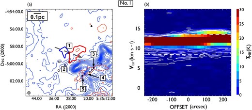
Same as in figure 7 but for outflow No. 1. In panel (a), the blueshifted and redshifted integrated intensity velocity ranges are |$0.0\:$|km|$\:$|s|$^{-1}$| to |$8.2\:$|km|$\:$|s|$^{-1}$| and |$13.2\:$|km|$\:$|s|$^{-1}$| to |$20.2\:$|km|$\:$|s|$^{-1}$|, respectively. (Color online)
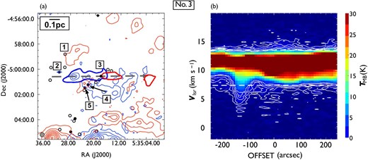
Same as in figure 7 but for outflow No. 3. In panel (a), the blueshifted and redshifted integrated intensity velocity ranges are |$0.0\:$|km|$\:$|s|$^{-1}$| to |$7.4\:$|km|$\:$|s|$^{-1}$| and |$13.6\:$|km|$\:$|s|$^{-1}$| to |$20.2\:$|km|$\:$|s|$^{-1}$|, respectively. (Color online)
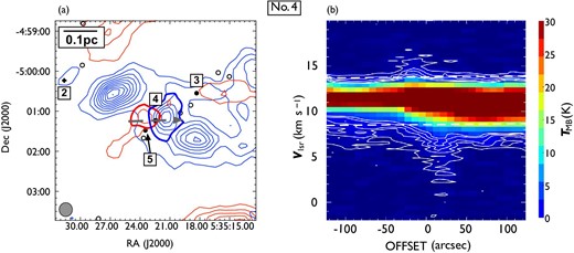
Same as in figure 7 but for outflow No. 4. In panel (a), the blueshifted and redshifted integrated intensity velocity ranges are |$0.0\:$|km|$\:$|s|$^{-1}$| to |$8.2\:$|km|$\:$|s|$^{-1}$| and |$13.8\:$|km|$\:$|s|$^{-1}$| to |$20.2\:$|km|$\:$|s|$^{-1}$|, respectively. (Color online)
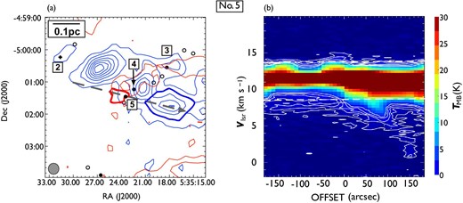
Same as in figure 7 but for outflow No. 5. In panel (a), the blueshifted and redshifted integrated intensity velocity ranges are |$0.0\:$|km|$\:$|s|$^{-1}$| to |$8.6\:$|km|$\:$|s|$^{-1}$| and |$14.0\:$|km|$\:$|s|$^{-1}$| to |$20.2\:$|km|$\:$|s|$^{-1}$|, respectively. (Color online)
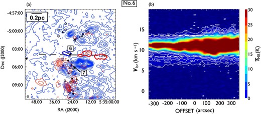
Same as in figure 7 but for outflow No. 6. In panel (a), the blueshifted and redshifted integrated intensity velocity ranges are |$0.0\:$|km|$\:$|s|$^{-1}$| to |$8.5\:$|km|$\:$|s|$^{-1}$| and |$13.5\:$|km|$\:$|s|$^{-1}$| to |$20.2\:$|km|$\:$|s|$^{-1}$|, respectively. (Color online)
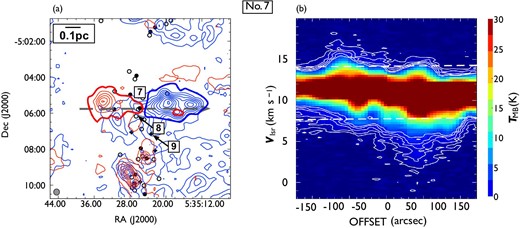
Same as in figure 7 but for outflow No. 7. In panel (a), the blueshifted and redshifted integrated intensity velocity ranges are |$0.0\:$|km|$\:$|s|$^{-1}$| to |$7.8\:$|km|$\:$|s|$^{-1}$| and 14.1 km|$\:$|s|$^{-1}$| to |$20.2\:$|km|$\:$|s|$^{-1}$|, respectively. (Color online)
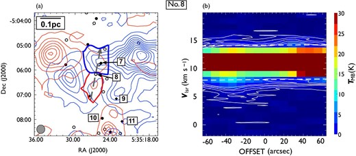
Same as in figure 7 but for outflow No. 8. In panel (a), the blueshifted and redshifted integrated intensity velocity ranges are |$0.0\:$|km|$\:$|s|$^{-1}$| to 8.1 km|$\:$|s|$^{-1}$| and 14.1 km|$\:$|s|$^{-1}$| to |$20.2\:$|km|$\:$|s|$^{-1}$|, respectively. (Color online)
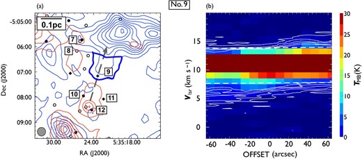
Same as in figure 7 but for outflow No. 9. In panel (a), the blueshifted and redshifted integrated intensity velocity ranges are |$0.0\:$|km|$\:$|s|$^{-1}$| to 7.6 km|$\:$|s|$^{-1}$| and |$13.8\:$|km|$\:$|s|$^{-1}$| to |$20.2\:$|km|$\:$|s|$^{-1}$|, respectively. (Color online)
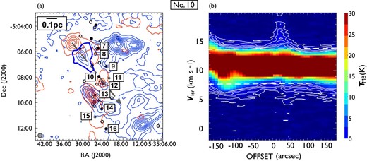
Same as in figure 7 but for outflow No. 10. In panel (a), the blueshifted and redshifted integrated intensity velocity ranges are |$0.0\:$|km|$\:$|s|$^{-1}$| to |$7.8\:$|km|$\:$|s|$^{-1}$| and 13.7 km|$\:$|s|$^{-1}$| to |$20.2\:$|km|$\:$|s|$^{-1}$|, respectively. (Color online)
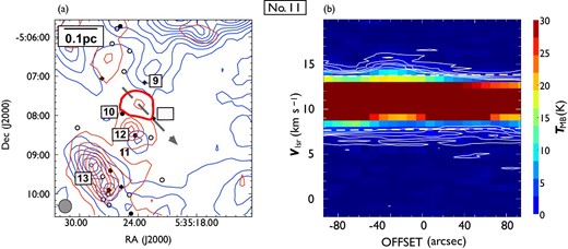
Same as in figure 7 but for outflow No. 11. In panel (a), the blueshifted and redshifted integrated intensity velocity ranges are |$0.0\:$|km|$\:$|s|$^{-1}$| to |$7.7\:$|km|$\:$|s|$^{-1}$| and |$13.8\:$|km|$\:$|s|$^{-1}$| to |$20.2\:$|km|$\:$|s|$^{-1}$|, respectively. (Color online)
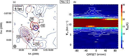
Same as in figure 7 but for outflow No. 12. In panel (a), the blueshifted and redshifted integrated intensity velocity ranges are |$0.0\:$|km|$\:$|s|$^{-1}$| to |$7.8\:$|km|$\:$|s|$^{-1}$| and |$13.5\:$|km|$\:$|s|$^{-1}$| to |$20.2\:$|km|$\:$|s|$^{-1}$|, respectively. (Color online)

Same as figure 7, but for outflow No. 13. In panel (a), the blueshifted and redshifted integrated intensity velocity ranges are |$0.0\:$|km|$\:$|s|$^{-1}$| to |$7.7\:$|km|$\:$|s|$^{-1}$| and |$14.2\:$|km|$\:$|s|$^{-1}$| to |$20.2\:$|km|$\:$|s|$^{-1}$|, respectively. (Color online)
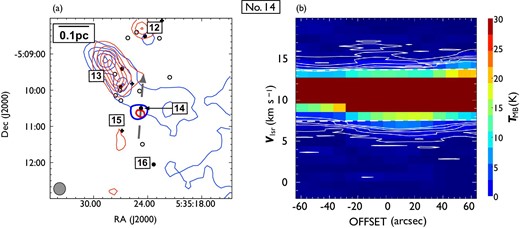
Same as in figure 7 but for outflow No. 14. In panel (a), the blueshifted and redshifted integrated intensity velocity ranges are |$0.0\:$|km|$\:$|s|$^{-1}$| to |$7.3\:$|km|$\:$|s|$^{-1}$| and |$13.6\:$|km|$\:$|s|$^{-1}$| to |$20.2\:$|km|$\:$|s|$^{-1}$|, respectively. (Color online)
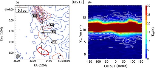
Same as in figure 7 but for outflow No. 15. In panel (a), the blueshifted and redshifted integrated intensity velocity ranges are |$0.0\:$|km|$\:$|s|$^{-1}$| to |$8.4\:$|km|$\:$|s|$^{-1}$| and |$13.3\:$|km|$\:$|s|$^{-1}$| to |$20.2\:$|km|$\:$|s|$^{-1}$|, respectively. The redshifted emission south of the central source is considered to be part of outflow No. 16. (Color online)
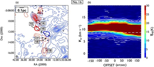
Same as in figure 7 but for outflow No. 16. In panel (a), the blueshifted and redshifted integrated intensity velocity ranges are |$0.0\:$|km|$\:$|s|$^{-1}$| to |$8.3\:$|km|$\:$|s|$^{-1}$| and |$13.2\:$|km|$\:$|s|$^{-1}$| to |$20.2\:$|km|$\:$|s|$^{-1}$|, respectively. (Color online)
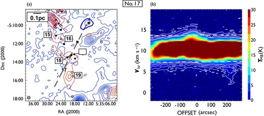
Same as in figure 7 but for outflow No. 17. In panel (a), the blueshifted and redshifted integrated intensity velocity ranges are |$0.0\:$|km|$\:$|s|$^{-1}$| to |$7.2\:$|km|$\:$|s|$^{-1}$| and |$13.6\:$|km|$\:$|s|$^{-1}$| to |$20.2\:$|km|$\:$|s|$^{-1}$|, respectively. The black cross represents the location of the emission peak of H|$_2$| jets detected by Davis et al. (2009). The position angle of outflows represented by the arrow in panel (a) and that of the H|$_2$| jet described by Davis et al. (2009) are in agreement. (Color online)
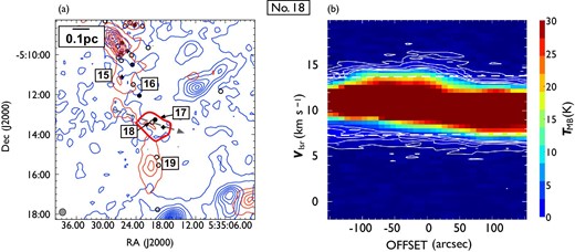
Same as in figure 7 but for outflow No. 18. In panel (a), the blueshifted and redshifted integrated intensity velocity ranges are |$0.0\:$|km|$\:$|s|$^{-1}$| to |$7.2\:$|km|$\:$|s|$^{-1}$| and |$13.6\:$|km|$\:$|s|$^{-1}$| to |$20.2\:$|km|$\:$|s|$^{-1}$|, respectively. (Color online)
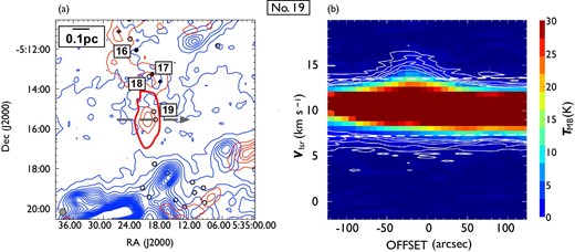
Same as in figure 7 but for outflow No. 19. In panel (a), the blueshifted and redshifted integrated intensity velocity ranges are |$0.0\:$|km|$\:$|s|$^{-1}$| to |$7.1\:$|km|$\:$|s|$^{-1}$| and |$13.5\:$|km|$\:$|s|$^{-1}$| to |$20.2\:$|km|$\:$|s|$^{-1}$|, respectively. (Color online)
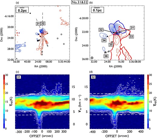
Same as in figure 7 but for outflow No. 31 and 32. In panel (a), the blueshifted and redshifted integrated intensity velocity ranges are |$-1.9\:$|km|$\:$|s|$^{-1}$| to |$3.8\:$|km|$\:$|s|$^{-1}$| and |$12.3\:$|km|$\:$|s|$^{-1}$| to |$20.2\:$|km|$\:$|s|$^{-1}$|, respectively. Panel (b) is a close up view of the center of panel (a). Panel (c) and (d) are the P–V diagrams of No. 31 and No. 32, respectively. (Color online)
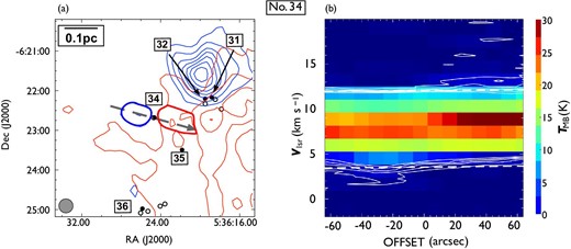
Same as in figure 7 but for outflow No. 34. In panel (a), the blueshifted and redshifted integrated intensity velocity ranges are |$-1.9\:$|km|$\:$|s|$^{-1}$| to |$3.4\:$|km|$\:$|s|$^{-1}$| and 1|$2.0\:$|km|$\:$|s|$^{-1}$| to |$20.2\:$|km|$\:$|s|$^{-1}$|, respectively. (Color online)

Same as in figure 7 but for outflow No. 35. In panel (a), the blueshifted and redshifted integrated intensity velocity ranges are |$-1.9\:$|km|$\:$|s|$^{-1}$| to 5.5 km|$\:$|s|$^{-1}$| and 11.4 km|$\:$|s|$^{-1}$| to |$18.0\:$|km|$\:$|s|$^{-1}$|, respectively. (Color online)
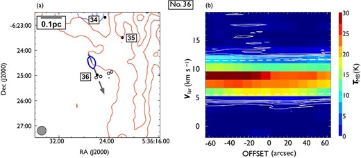
Same as in figure 7 but for outflow No. 36. In panel (a), the blueshifted and redshifted integrated intensity velocity ranges are |$-1.9\:$|km|$\:$|s|$^{-1}$| to |$3.4\:$|km|$\:$|s|$^{-1}$| and |$11.9\:$|km|$\:$|s|$^{-1}$| to |$18.0\:$|km|$\:$|s|$^{-1}$|, respectively. (Color online)
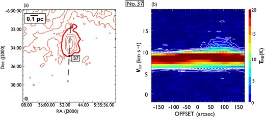
Same as in figure 7 but for outflow No. 39. In panel (a), the blueshifted and redshifted integrated intensity velocity ranges are |$-1.9\:$|km|$\:$|s|$^{-1}$| to |$4.9\:$|km|$\:$|s|$^{-1}$| and |$10.4\:$|km|$\:$|s|$^{-1}$| to |$18.0\:$|km|$\:$|s|$^{-1}$|, respectively. (Color online)
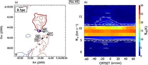
Same as in figure 7 but for outflow No. 40. In panel (a), the blueshifted and redshifted integrated intensity velocity ranges are |$-1.9\:$|km|$\:$|s|$^{-1}$| to |$4.8\:$|km|$\:$|s|$^{-1}$| and 11.6 km|$\:$|s|$^{-1}$| to |$18.0\:$|km|$\:$|s|$^{-1}$|, respectively. (Color online)
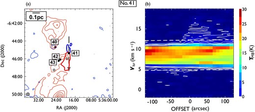
Same as in figure 7 but for outflow No. 41. In panel (a), the blueshifted and redshifted integrated intensity velocity ranges are |$-1.9\:$|km|$\:$|s|$^{-1}$| to 4.9 km|$\:$|s|$^{-1}$| and |$12.1\:$|km|$\:$|s|$^{-1}$| to |$20.2\:$|km|$\:$|s|$^{-1}$|, respectively. (Color online)
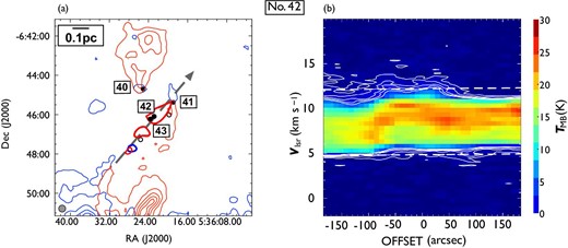
Same as in figure 7 but for outflow No. 42. In panel (a), the blueshifted and redshifted integrated intensity velocity ranges are |$-1.9\:$|km|$\:$|s|$^{-1}$| to |$4.8\:$|km|$\:$|s|$^{-1}$| and |$12.1\:$|km|$\:$|s|$^{-1}$| to |$20.2\:$|km|$\:$|s|$^{-1}$|, respectively. (Color online)
References
