


Abstract
The star S0-2, orbiting the Galactic central massive black hole candidate Sgr A|$^\ast$|, passed its pericenter in 2018 May. This event is the first chance to detect the general relativistic (GR) effect of a massive black hole, free from non-gravitational physics. The observable GR evidence in the event is the difference between the GR redshift and the Newtonian redshift of photons coming from S0-2. Within the present observational precision, the first post-Newtonian (1PN) GR evidence is detectable. In this paper, we give a theoretical analysis of the time evolution of the 1PN GR evidence, under a presupposition that is different from used in previous papers. Our presupposition is that the GR/Newtonian redshift is always calculated with the parameter values (the mass of Sgr A|$^\ast$|, the initial conditions of S0-2, and so on) determined by fitting the GR/Newtonian motion of S0-2 with the observational data. It is then revealed that the difference of the GR redshift and the Newtonian one shows two peaks before and after the pericenter passage. This double-peak appearance is due to our presupposition, and reduces to a single peak if the same parameter values are used in both GR and Newtonian redshifts as considered in previous papers. In addition to this theoretical discussion, we report our observational data obtained with the Subaru telescope by 2018. The quality and the number of Subaru data in 2018 are not sufficient to confirm the detection of the double-peak appearance.
1 Introduction
The general relativistic (GR) effect has already been distinguished observationally from non-GR effects, for example, in the following situations: the weak gravity in our solar system (e.g., Will 2014), the cosmic microwave background radiation (e.g., Hinshaw et al. 2013 and Planck Collaboration 2018), and the gravitational waves radiated by stellar-size compact objects (e.g., Abbott et al. 2016). However, the GR effect of massive black holes (BHs) remains to be distinguished observationally from non-GR effects. A good probe of the quantitative assessment of GR effect of a massive BH is the star called S0-2 (in the Keck nomenclature) or S2 (in the very large telescope, VLT, nomenclature), that is orbiting Sgr A|$^\ast$| (of mass |${\approx} 4\times 10^6\, M_\odot$|), with an orbital period of |${\approx} 16\:$|yr and a closest distance to Sgr A|$^\ast$| of |${\approx} 100\:$|au. Because S0-2 is regarded as a test particle moving in the gravitational field of Sgr A|$^\ast$|, the motion of S0-2 provides us with the pure GR effect free from non-gravitational physics (Zucker et al. 2006). Measurements of the pure GR effect in the motion of S0-2 will enable us to test GR in the strong gravitational field of Sgr A|$^\ast$|.1
Monitoring observations of the S0-2 motion can be performed by a few groups using large telescopes such as VLT, Keck, Gemini and Subaru. We have been monitoring the redshift of photons emitted by S0-2 from 2014 using Subaru (Nishiyama et al. 2018), and American and European groups have been monitoring the position and redshift of S0-2 for about 20 years using other telescopes (Boehle et al. 2016; Gillessen et al. 2017; Parsa et al. 2017; Chu et al. 2018; GRAVITY collaboration 2018, 2019; Do et al. 2019). Until 2017, those observations had not revealed a clear deviation from the prediction of Newtonian gravity in the S0-2 motion. However, it has been expected that the deviation from the Newtonian prediction would become detectable in the redshift of photons coming from S0-2 during its pericenter passage in 2018 (e.g., Zucker et al. 2006). Recently, a detection of the combination of the special relativistic and gravitational Doppler effects has been reported by a European group (GRAVITY collaboration 2018) and by an American group (Do et al. 2019).
The evidence of GR being explored using the large telescopes is theoretically expressed as the difference between the redshift predicted by GR and the one predicted by Newtonian gravity. Within the present observational precision, this GR evidence is detectable at the first post-Newtonian order. The redshift depends on some parameters, for example, the mass of Sgr A|$^\ast$| and the initial conditions of the S0-2 motion. In this paper, we adopt the following presupposition on the treatment of the parameter values;
Presupposition: The GR redshift is always calculated with the best-fitting parameter values determined by fitting the GR motion of S0-2 with the observational data. The Newtonian redshift is always calculated with the best-fitting parameter values determined by fitting the Newtonian motion of S0-2 with the observational data.
The GR best-fitting values and the Newtonian ones are different. In order to confirm the validity of GR for the gravitational field of Sgr A|$^\ast$|, it is useful to search for evidence of GR in the difference between the two best fits. In this paper, we report the time evolution of the difference between GR redshift and Newtonian redshift. Under our presupposition, it shows two peaks before and after the pericenter passage of S0-2. This “double-peak appearance” has not been reported so far in previous papers (e.g., GRAVITY collaboration 2018; Do et al. 2019). In the previous papers, the same parameter values, which have been carefully determined, have been used in both GR and Newtonian redshifts (see subsection 2.3), and then the resultant single-peak behavior has been discussed. If the GR is favored by two different approaches, such as the approach of the previous papers and the one under our presupposition, then the GR can be favored more definitely than the case using only one approach.
As a by-product of our presupposition, it is found that the statistical quantity |$\chi _{\rm red}^2$|, called the “reduced-chi-squared”, is not useful for discriminating between GR and Newtonian gravity within the present observational precision. Therefore, instead of the |$\chi _{\rm red}^2$|, we propose another quantity, denoted as |$\delta z$| in this paper (subsection 4.3), which expresses to what extent the double-peak appearance determined by the observational data matches well with the theoretically expected form of the double-peak appearance. Furthermore, in this paper, we report our observational data obtained by the Subaru telescope in 2017 and 2018, together with the data already reported in our previous paper (Nishiyama et al. 2018). Due to bad weather conditions and instrumental instabilities, the quality and the number of the data in 2018 are not sufficient to confirm the detection of the double-peak appearance, where the detection error is about |$60\%$| according to our quantity |$\delta z$|. We need additional data sets to confirm the detection of the double-peak appearance.
Section 2 is devoted to the theoretical discussion to derive the “double-peak appearance” in the time evolution of the difference between the GR redshift and the Newtonian one under our presupposition. The non-usefulness of |$\chi _{\rm red}^2$| for discriminating the GR and the Newtonian gravity within the present observational precision is also discussed. Section 3 is the summary of our observations of S0-2 using the Subaru telescope from 2014 to 2018. In section 4, the best fit of the double-peak appearance with our observational data is presented, and the quality of our 2018 data is also shown. Then, we introduce the quantity |$\delta z$|, which measures the discrepancy between the GR and the Newtonian gravity under our presupposition. Section 5 is the summary and discussion.
2 Theoretically expected time evolution of the GR evidence under our presupposition
2.1 Definitions
The set-up of the coordinate system has to be clarified. The detail of it is explained in appendix 1, and here let us summarize an important point: Our definitions of some quantities, for example the Roemer time delay, are not exactly the same as those used in previous papers (GRAVITY collaboration 2018; Do et al. 2019). For example, we always take into account the finiteness of the distance between Sun and Sgr A|$^\ast$| in calculating the Roemer time delay, while the time delay in the previous papers is approximated by the infinite distance limit. However, under the present observational uncertainties, such differences in the definitions of some quantities are not detectable.
2.2 Post-Newtonian and post-Minkowskian approximations within observational precision
Full GR formulation has a high numerical cost. In order to reduce the cost, we use the post-Newtonian (PN) and post-Minkowskian (PM) approximations (e.g., Poisson & Will 2014) of the S0-2 motion and photon propagation. Some numerical simulations for PN and PM approximations have been shown in Angélil and Saha (2010) and Angélil, Saha, and Merritt (2010). However, without those simulations, we can justify the first-order PN (1PN) approximation for the S0-2 motion and the 0th order PM (0PM) approximation for the photon propagation within the present observational precision.
For the motion of the observer, we can ignore the GR effect because of the huge distance to Sgr A|$^\ast$| from us |$\simeq 8\:$|kpc. We assume the velocity of the observer is constant.
The above discussions justify the 1PN approximation for the S0-2 motion and the 0PM approximation for the photon propagation. Hereafter, the combination of these approximations is phrased as the “1PN|$\, +\,$|0PM” approximation. Throughout this paper, the 1PN|$\, +\,$|0PM approximation is used under the assumption of the constant velocity of the observer.
Some details on |$\Delta z_{\rm 1PN.0PM}(t)$| are analyzed in subsection 2.2 of appendix 2; here, let us summarize an important point. The first and second terms in |$\Delta z_{\rm 1PN.0PM}(t)$|, which are the difference between the line-of-sight velocities of GR and Newtonian cases, do not necessarily vanish and have to be counted as the non-vanishing components in |$\Delta z_{\rm 1PN.0PM}(t)$| under our presupposition. The reason is that the best-fitting values of parameters (e.g., the Sgr A|$^\ast$|’s mass and the S0-2’s initial conditions) in the GR case is different from those in the Newtonian case, and hence the same quantities in both GR and Newtonian cases, such as the line-of-sight velocities of S0-2 and the observer, take different values in the GR and Newtonian cases.
2.3 On the quantity that measures the difference between the GR and Newtonian predications
Given the observational data, calculate |$\Delta z_{\rm 1PN.0PM}(t)$| under our presupposition. Then, the closer the time evolution of |$\Delta z_{\rm 1PN.0PM}(t)$| to the theoretically expected time evolution of it, the more definite the detection of the difference between the GR and Newtonian predictions.
Here, the point in this assessment is how we can estimate the theoretically expected time evolution of |$\Delta z_{\rm 1PN.0PM}(t)$|. The next subsection is devoted to this point.
In equation (16), the parameter f is introduced by hand, while the geodesic equations of S0-2 (and of photons) are not modified by introducing the parameter f. This parametrization is different from the so-called parametrized-post-Newtonian (PPN) formalism, which is the parametrization of the spacetime metric tensor at the 1PN order and causes some modifications not only of the redshift of photons but also of the S0-2 motion. Because this f is not exactly a parametrization used widely in the usual PPN formalism, the parameter f is interpreted as an ad-hoc or a highly specialized parameter to measure the combination of the special relativistic and gravitational Doppler effects.
Let the GR motion of S0-2 be substituted in |$z_{\rm GR}^{\rm (prev)}$|. Then, the case of |$f=1$| denotes the GR case, because |$\Delta z_{\rm GR}^{\rm (prev)}$| with |$f=1$| is exactly the combination of the special relativistic and gravitational Doppler effects at the 1PN|$\, +\,$|0PM order. However, the case of |$f=0$| never denotes a Newtonian case, because the “GR motion” of S0-2 is substituted in |$z_{\rm GR}^{\rm (prev)}$|. In general, the case of |$f\ne 1$| is not a modified theory of gravity, because the S0-2 motion is the pure GR case (i.e., the gravity is not modified for the S0-2 motion) while only the redshift formula is modified by introducing f.
From the above two points, the introduction of f into |$z_{\rm GR}^{\rm (prev)}$| can be interpreted as the assessment of the hypothesis that the gravitational field of Sgr A|$^\ast$| is described by GR (neither Newtonian gravity nor a modified theories of gravity). When the value of f is determined by fitting the observational data with |$z_{\rm GR}^{\rm (prev)}$| together with the GR motion of S0-2, the closer the best-fitting value of f to unity, the more plausible the hypothesis that the Sgr A|$^\ast$|’s gravity is GR.
The quantity |$\Delta z_{\rm GR}^{\rm (prev)}$| is not a deviation from Newtonian prediction, but the measure to assess the “GR hypothesis”. GRAVITY collaboration (2018) has reported the best-fitting value of |$f = 0.945\pm 0.090$| using GRAVITY data from 2018, and Do et al. (2019) has reported the best-fitting value of |$f = 0.88\pm 0.16$| using Keck, Gemini, and Subaru data from 2018. The evidence of GR has been found through the assessment of the GR hypothesis.
Both quantities |$\Delta z_{\rm 1PN.0PM}$| and |$\Delta z_{\rm GR}^{\rm (prev)}$| can assess the validity of GR as the theory of gravity near Sgr A|$^\ast$|, although the exact meanings of these quantities are different. Our quantity |$\Delta z_{\rm 1PN.0PM}$| focuses on the total deviation of the GR prediction from the Newtonian prediction under our presupposition. The quantity in the previous papers |$\Delta z_{\rm GR}^{\rm (prev)}$| focuses on the combination of the special relativistic and gravitational Doppler effects, excluding the difference of the time evolution of S0-2’s velocity between the GR and Newtonian cases. Note that, if the GR is favored by two different approaches, such as the approach of the previous papers and the one introduced in this paper, then the GR can be favored more definitely than the case favored by only one approach. Our approach does not conflict with the approach of the previous papers, but provides us with an additional reference for confirming the validity of GR.4
2.4 Expected time evolution of |$\Delta z_{\rm 1PN.0M}$| for ideally accurate observational data
The theoretically expected time evolution of |$\Delta z_{\rm 1PN.0PM}(t)$| is the key issue in this paper. Let us introduce a condition:
Condition (ideally accurate data set):An ideally accurate observational data set is given. Here, the term “ideally accurate” denotes that (i) the error assigned to each data is constant for all observation times, and (ii) the observational value itself takes exactly the same value as the GR prediction, where the offset of the astrometric origin is zero.
Under this condition, we define the theoretically expected time evolution of |$\Delta z_{\rm 1PN0PM}(t)$| as the one derived by the following steps:
Step 1: Fix the values of all parameters which are listed in sub-subsection 2.4.1. Using these values, calculate the GR motion of S0-2, |$x_{\rm S.1PN}^\mu (\tau )$|, and the GR redshift, |$z_{\rm 1PN.0PM}(t)$|, at the 1PN|$\, +\,$|0PM approximation.
Step 2: Artificially create the ideally accurate data set, in which every value of RA, Dec and redshift (|$z_{\rm 1PN.0PM}$|) of S0-2 are exactly the same as the GR prediction given in step 1, and the astrometric offset defined in equation (A3) is zero, |$\boldsymbol {A}_{\rm sky} \equiv \boldsymbol {0}$|. Let the error assigned to each data be the averaged error of real observational data.
Step 3: By fitting the artificial data with the Newtonian motion of S0-2, calculate the Newtonian best-fitting values of all parameters listed in sub-subsection 2.4.1. Such Newtonian best-fitting parameter values are not necessarily equal to the parameter values used in step 1. Then, calculate the Newtonian redshift, |$z_{\rm NG}(t)$|, using the Newtonian best-fitting parameter values.
Step 4: From steps 1 and 3, calculate the time evolution of the quantity, |$\Delta z_{\rm 1PN.0PM}(t) = z_{\rm 1PN.0PM}(t)-z_{\rm NG}(t)$|. This is interpreted as the theoretically expected time evolution of the difference between the GR and Newtonian redshifts under our presupposition on the parameter values.
In following subsections, we will carry out these steps.
2.4.1 Step 1: Parameter values for GR prediction
As examples, let us use two sets of best-fitting parameter values given in Boehle et al. (2016) and GRAVITY collaboration (2018). Those values are shown in table 1, where the definitions of the 11 parameters are:
|$M_{\rm SgrA}$|: the mass of Sgr A|$^\ast$|.
|$R_{\rm GC}$|: the distance between Sun and Sgr A|$^\ast$|.
|$V_{\rm O.ra}$|: the Y (RA)-component of the observer’s velocity |$\boldsymbol {V}_{\rm O}$| relative to Sgr A|$^\ast$|, see equation (A2).
|$V_{\rm O.dec}$|: the X (Dec)-component of the observer’s velocity |$\boldsymbol {V}_{\rm O}$| relative to Sgr A|$^\ast$|, see equation (A2).
|$V_{\rm O.Z}$|: the Z-component of the observer’s velocity |$\boldsymbol {V}_{\rm O}$| relative to Sgr A|$^\ast$|, see equation (A2).
|$I_{\rm S}$|: the inclination angle of the orbital plane of S0-2, when it is evaluated in the Newtonian motion.
|$\Omega _{\rm S}$|: the angle of ascending node from Dec direction on the orbital plane of S0-2, when it is evaluated in the Newtonian motion.
|$\omega _{\rm S}$|: the angle of pericenter node from the ascending node on the orbital plane of S0-2, when it is evaluated in the Newtonian motion.
|$e_{\rm S}$|: the eccentricity of the S0-2 orbit, when it is evaluated in the Newtonian motion.
|$T_{\rm S}$|: the orbital period of S0-2 around Sgr A|$^\ast$|, when it is evaluated in the Newtonian motion.
|$t_{\rm S.apo}$|: the time of the previous apocenter passage in 2010.
Two examples of parameter values with which GR motions are calculated.
| Parameters for Sgr A|$^\ast$| and observer | |$M_{\rm SgrA}$| | |$R_{\rm GC}$| | |$V_{\rm O.ra}$| | |$V_{\rm O.dec}$| | |$V_{\rm O.Z}$| | — |
|---|---|---|---|---|---|---|
| [|$10^6\, M_\odot$|] | [kpc] | [mas|$\:$|yr|$^{-1}$|] | [mas|$\:$|yr|$^{-1}$|] | [km|$\:$|s|$^{-1}$|] | — | |
| Boehle et al. (2016) | 4.12 | 8.02 | 0.02 | |$-$|0.55 | |$-$|15 | — |
| GRAVITY collaboration (2018) | 4.100 | 8.122 | |$-$|0.076 | |$-$|0.178 | 1.9 | — |
| Parameters for S0-2 orbit | |$I_{\rm S}$| | |$\Omega _{\rm S}$| | |$\omega _{\rm S}$| | |$e_{\rm S}$| | |$T_{\rm S}$| | |$t_{\rm S.apo}$| |
| [|$^{\circ }$|] | [|$^{\circ }$|] | [|$^{\circ }$|] | [no dim.] | [yr] | [AD] | |
| Boehle et al. (2016) | 134.7 | 227.9 | 66.5 | 0.890 | 15.90 | 2010.293 |
| GRAVITY collaboration (2018) | 133.818 | 227.85 | 66.13 | 0.88466 | 16.0518 | 2010.35384 |
Here we need to note two remarks. The first remark is on the artificial data that will be created in step 2. We define the artificial data as the ideally accurate data in which the astrometric offset defined in equation (A3) is not introduced, |$\boldsymbol {A}_{\rm sky}(t) \equiv \boldsymbol {0}$|. Therefore, in table 1, the parameters corresponding to |$\boldsymbol {A}_{\rm sky}(t)$| are not included.
The second remark is on the last six parameters, from |$I_{\rm S}$| to |$t_{\rm S.apo}$|. Although these six parameters are given in the form of orbital elements of the Newtonian motion, it does never mean that these six parameters are available only for the Newtonian motion. In solving the geodesic equations (6) of the S0-2 motion, we simply transform those six parameters to the initial conditions, position and velocity, given at the time |$t_{\rm S.apo}$|. We regard those six parameters, from |$I_{\rm S}$| to |$t_{\rm S.apo}$|, as the control parameters of the initial conditions for the GR motion. Hence, if the GR motion is given (for example, from the best-fitting calculation), then the position and velocity of S0-2 at the apocenter are transformed to the six parameters, |$I_{\rm S}$| to |$t_{\rm S.apo}$| by simple Newtonian formulas of these six parameters.
2.4.2 Step 2: Ideally accurate data set
For each set of parameter values in table 1, we create the ideally accurate data set under the following conditions:
Condition 1: Create N data of RA, Dec, and |$cz_{\rm 1PN.0PM}$| per year with a constant temporal interval, |$1/N\:$|yr.
Condition 2: Create the data set corresponding to L years’ observations, where L is sufficiently longer than one period, |$T_{\rm S}$|, in order to follow the whole time evolution of |$z_{\rm GR}(t)$| in one period.5 This L needs to be short enough to make the shift of the pericenter/apocenter angle be significantly smaller than |$90^\circ$|, because a large shift of the angle causes a significant change in the observed time evolution of |$z_{\rm GR}(t)$|.
Condition 3: As noted at the beginning of this subsection 2.4, the error assigned to each data is the averaged error of real observational data. The error in RA observation is |$9.832\times 10^{-4}\:$|arcsec, in Dec observation |$9.176\times 10^{-4}$|, and in redshift (times the light speed, |$c z_{\rm GR}$|) observation |$38.29\:$|km|$\:$|s|$^{-1}$|, which are read from the public data in Boehle et al. (2016), GRAVITY collaboration (2018), and our observations listed in table 4.
The number of each kind of data, RA, Dec, and |$cz_{\rm 1PN.0PM}$|, is |$NL$| (i.e., |$3NL$| data in total). In the following numerical calculations, we set |$L=4 T_{\rm S} \approx\! 64\:$|yr, during an interval |$t_{\rm S.apo}-2T_{\rm S} \lt t \lt t_{\rm S.apo}+2T_{\rm S}$|, centered at the previous apocenter time in 2010. This duration of |$4T_{\rm S}$| corresponds to the angle of pericenter/apocenter shift |$\approx\! 4\times 6\pi GM_{\rm SgrA}/(c^2 r_{\rm S}) \sim 4^\circ$|, which is sufficiently smaller than |$90^\circ$|. Further, we consider three cases of the number of data per year, |$N = 10,\, 15,\, 20$|, where |$N=15$| is roughly the averaged number of observations per year until 2017. Because we consider three values of N for each example of parameters in table 1, we have six cases of artificial data sets. For these cases, we are going to calculate the expected time evolution of |$\Delta z_{\rm 1PN0PM}$| under our presupposition on the parameter values. Our numerical calculations are performed using Mathematica, version 11.
2.4.3 Step 3: Fitting with Newtonian prediction
Best fit of Newtonian motion of S0-2 with each data set created in step 2.|$^*$|
| |$\chi _{\rm red.min}^2$| and parameters | |$\chi _{\rm red.min}^2$| | |$M_{\rm SgrA}$| | |$R_{\rm GC}$| | |$V_{\rm O.ra}$| |
|---|---|---|---|---|
| determined by |$\chi ^2$|-fitting | [no dim.] | [|$10^6\, M_\odot$|] | [kpc] | [mas|$\:$|yr|$^{-1}$|] |
| Boehle et al., |$N=10$| | 0.0751 | |$4.235\pm 0.028$| | |$8.126\pm 0.026$| | |$0.054\pm 0.002$| |
| Boehle et al., |$N=15$| | 0.0739 | |$4.232\pm 0.023$| | |$8.123\pm 0.021$| | |$0.054\pm 0.002$| |
| Boehle et al., |$N=20$| | 0.0739 | |$4.231\pm 0.020$| | |$8.122\pm 0.018$| | |$0.054\pm 0.002$| |
| GRAVITY collaboration, |$N=10$| | 0.0689 | |$4.208\pm 0.027$| | |$8.223\pm 0.025$| | |$-0.045\pm 0.002$| |
| GRAVITY collaboration, |$N=15$| | 0.0687 | |$4.205\pm 0.022$| | |$8.220\pm 0.020$| | |$-0.045\pm 0.002$| |
| GRAVITY collaboration, |$N=20$| | 0.0687 | |$4.205\pm 0.019$| | |$8.220\pm 0.018$| | |$-0.045\pm 0.002$| |
| Parameters | |$V_{\rm O.dec}$| | |$V_{\rm O.Z}$| | |$I_{\rm S}$| | |$\Omega _{\rm S}$| |
| [mas|$\:$|yr|$^{-1}$|] | [km|$\:$|s|$^{-1}$|] | [|$^{\circ }$|] | [|$^{\circ }$|] | |
| Boehle et al., |$N=10$| | |$-0.533\pm 0.002$| | 2.484 |$\pm$| 1.512 | |$134.764\pm 0.084$| | |$227.106\pm 0.096$| |
| Boehle et al., |$N=15$| | |$-0.533\pm 0.002$| | |$2.422\pm 1.235$| | |$134.756\pm 0.067$| | |$227.113\pm 0.078$| |
| Boehle et al., |$N=20$| | |$-0.533\pm 0.001$| | |$2.423\pm 1.070$| | |$134.754\pm 0.058$| | |$227.115\pm 0.067$| |
| GRAVITY collaboration, |$N=10$| | |$-0.163\pm 0.002$| | |$19.029\pm 1.512$| | |$133.872\pm 0.078$| | |$227.111\pm 0.092$| |
| GRAVITY collaboration, |$N=15$| | |$-0.163\pm 0.002$| | |$19.228\pm 1.235$| | |$133.863\pm 0.064$| | |$227.122\pm 0.075$| |
| GRAVITY collaboration, |$N=20$| | |$-0.163\pm 0.001$| | |$19.248\pm 1.070$| | |$133.863\pm 0.055$| | |$227.122\pm 0.065$| |
| Parameters | |$\omega _{\rm S}$| | |$e_{\rm S}$| | |$T_{\rm S}$| | |$t_{\rm S.apo}$| |
| [|$^{\circ }$|] | [no dim.] | [yr] | [AD] | |
| Boehle et al., |$N=10$| | |$65.817\pm 0.091$| | 0.8896 |$\pm$| 0.0003 | 15.8985 |$\pm$| 0.0004 | 2010.2956 |$\pm$| 0.0005 |
| Boehle et al., |$N=15$| | |$65.826\pm 0.073$| | 0.8896 |$\pm$| 0.0002 | 15.8985 |$\pm$| 0.0003 | 2010.2958 |$\pm$| 0.0004 |
| Boehle et al., |$N=20$| | |$65.828\pm 0.063$| | |$0.8896\pm 0.0002$| | |$15.8985\pm 0.0003$| | |$2010.2958\pm 0.0003$| |
| GRAVITY collaboration, |$N=10$| | |$65.497\pm 0.087$| | |$0.8842\pm 0.0003$| | |$16.0505\pm 0.0004$| | |$2010.3566\pm 0.0005$| |
| GRAVITY collaboration, |$N=15$| | |$65.510\pm 0.071$| | |$0.8842\pm 0.0002$| | |$16.0503\pm 0.0003$| | |$2010.3567\pm 0.0004$| |
| GRAVITY collaboration, |$N=20$| | |$65.510\pm 0.061$| | |$0.8842\pm 0.0002$| | |$16.0503\pm 0.0003$| | |$2010.3567\pm 0.0004$| |
|$^*$| N is the number of data per year, for each of RA, Dec, and |$cz$|. The error in |$\chi ^2$|-fitting is given by definition (18).
Before proceeding to step 4, let us remark an implication of the very small value of |$\chi _{\rm red.min}^2\approx\! 0.07$| in table 2. Because table 2 is made from the ideally accurate data sets, the |$\chi _{\rm red.min}^2$| in table 2 can be interpreted as one quantity that measures a discrepancy between GR and Newtonian gravity under the idea of |$\chi ^2$|-assessment.6 Therefore, if |$\chi _{\rm red.min}^2$| in table 2 was of the order of one or more, |$\chi _{\rm red.min}^2\gtrsim O(1)$|, then it was expected that we would be able to confirm the detection of |$\Delta z_{\rm 1PN.0PM}(t)$| by the |$\chi ^2$|-assessment. In other words, the small value |$\chi _{\rm red.min}^2\approx\! 0.07$| in table 2 implies that the |$\chi ^2$|-assessment does not work well for a detection of |$\Delta z_{\rm 1PN.0PM}(t)$|, even if very accurate observations would be performed with the present observational precision.
2.4.4 Step 4: Theoretically expected time evolution of our GR evidence |$\Delta z_{\rm 1PN.0PM}(t)$|
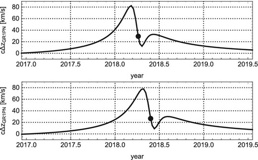
The parameter values in tables 1 and 2 provide us with a theoretically expected time evolution of |$\Delta z_{\rm 1PN.0PM}(t)$|. In this paper, all figures of redshift are shown in the unit of km|$\:$|s|$^{-1}$|, by multiplying the light speed as |$cz(t)$|.
Figure 1 shows the theoretically expected time evolution of the redshift of photons coming from S0-2 at the 1PN|$\, +\,$|0PM approximation, |$cz_{\rm 1PN.0PM}(t)$| in equation (11), using the parameter values in table 1. The top panel is for the case of Boehle et al. (2016), and the bottom panel for the case of GRAVITY collaboration (2018). Hereafter, the dots attached on curves in the figures denote the pericenter and apocenter passages of S0-2 estimated by the 1PN|$\, +\,$|0PM approximation, not by the Newtonian case. The pericenter time in the Newtonian case is delayed slightly by |$0.002\:$|yr |$\approx\! 0.7\:$|d after the pericenter time in the 1PN|$\, +\,$|0PM approximation.7 Note that, because the parameter values in GRAVITY collaboration (2018) are based on observations until June 2018 while those in Boehle et al. (2016) are based on observations until 2013, we find a horizontal shift between the top and bottom panels in figure 1. The discrepancy probably arises from the five-year difference of the observations. However, this discrepancy does not affect the result of this section.

Under our presupposition on the treatment of the parameter values, figure 2 shows the theoretically expected time evolution of |$c \Delta z_{\rm 1PN.0PM}(t)$|. The upper and bottom panels correspond, respectively, to the cases of Boehle et al. with |$N=20$| and GRAVITY collaboration with |$N=10$| in table 2. It is significant that the two peaks appear before and after the pericenter passage in both panels. Although a horizontal shift is recognized between the two panels, as already seen in figure 1, the “double-peak appearance” is not affected by the horizontal shift between the two panels. The time evolution of |$c \Delta z_{\rm 1PN.0PM}(t)$| for the other set of parameters in table 2 also shows the very similar “double-peak appearance”, although that is not presented here.
Theoretically expected time evolution of |$c \Delta z_{\rm 1PN.0PM}(t)$|. The top panel is for the case of Boehle et al. with |$N=20$| in table 2. The bottom panel is for the case of GRAVITY collaboration with |$N=10$| in table 2. Dots on the curves denote the pericenter passage of S0-2 estimated by the 1PN|$\, +\,$|0PM approximation. All other cases in table 2 show almost the same behavior.
In order to understand the origin of the “double-peak appearance”, it is useful to consider each component of |$c \Delta z_{\rm 1PN.0PM}(t)$| defined in equation (14). As an example, we focus on the case of GRAVITY collaboration with |$N=10$| in table 2.
![Decomposition of $\Delta z_{\rm 1PN.0PM}$ into two components. The top panel is for the theoretically expected time evolution of the sum of the third and fourth terms in equation (14) [$\Delta v_{\rm S}^2/(2c)+GM_{\rm SgrA}/(cr_{\rm S})$]. The bottom panel is for the theoretically expected time evolution of the sum of the first and second terms in equation (14) (noted as $\Delta$LSV in the panel). Both panels are drown with the case of GRAVITY collaboration with $N=10$. Dots on the curves denote the pericenter passage of S0-2 estimated by the 1PN$\, +\,$0PM approximation.](https://oup.silverchair-cdn.com/oup/backfile/Content_public/Journal/pasj/71/6/10.1093_pasj_psz111/2/m_pasj_71_6_126_f5.jpeg?Expires=1750215951&Signature=uwQ3HmmqpJG4ovUinWJjoRSItgk0Wf-47yIj7tGdehE8XiZFY1tA9oOrXN10QiBcayvS~Ezq2353XNgu8UjSYuttMZr6ChhQnDnCCNk2OF7JGQ9m5HB8kW27Ep0RwVNZ4yZl365yFixl4pUFgEzmZj7qyftlxS1d11t7wKDEIV3h7U~AAmesi6M5~BwX-XwnukiPxf07Y3p~a~bVSQT1RijQ93gCRC-ved7Gcy8FMn1rN3HIDltj9nuoEj4YzaKRK~wVxUUJTHLpHLd0zPwK5Y2vi7XsbRkEDvs4UtL6HSKY2YYHuNXG-AetJ9CRM2NNg-W59MG3UaZ9z6DRUpikLQ__&Key-Pair-Id=APKAIE5G5CRDK6RD3PGA)
Decomposition of |$\Delta z_{\rm 1PN.0PM}$| into two components. The top panel is for the theoretically expected time evolution of the sum of the third and fourth terms in equation (14) [|$\Delta v_{\rm S}^2/(2c)+GM_{\rm SgrA}/(cr_{\rm S})$|]. The bottom panel is for the theoretically expected time evolution of the sum of the first and second terms in equation (14) (noted as |$\Delta$|LSV in the panel). Both panels are drown with the case of GRAVITY collaboration with |$N=10$|. Dots on the curves denote the pericenter passage of S0-2 estimated by the 1PN|$\, +\,$|0PM approximation.
The point in the LSV component (20) is that, as indicated by the bottom panel of figure 3, the LSV of S0-2 in the Newtonian best-fitting case becomes faster than the LSV in the GR case, |$V_{\rm S.NG\parallel } \gt V_{\rm S.1PN\parallel }$|, around the pericenter passage. This is reasonable due to the following facts:
In general, the |$\chi ^2$|-fitting provides us with the parameter values that minimize the discrepancy between theory and data. Therefore, all sets of parameter values in table 2 must be adjusted so that the orbit and redshift of S0-2 in the Newtonian case become as similar as possible to those in the GR case.
The Newtonian redshift, |$cz_{\rm NG}(t)$| in equation (3), includes no counter-term to the “special relativistic and gravitational Doppler” component (19).
By facts (i) and (ii), it is expected that the motion of S0-2 with the Newtonian best-fitting parameter values is adjusted so as to compensate the special relativistic and gravitational Doppler component (19). Further, because of fact (ii), it is only the LSV component |$V_{\rm S.NG\parallel }(t+t_{\rm R})$| in the Newtonian motion of S0-2 that can compensate the special relativistic and gravitational Doppler component. Hence, as shown in figure 3, the LSV component (20) takes the negative value |$\approx\! -200\:$|km|$\:$|s|$^{-1}$| (bottom panel of figure 3) so as to compensate the positive value |$\approx\! 200\:$|km|$\:$|s|$^{-1}$| of the special relativistic and gravitational Doppler component (top panel of figure 3). This means that the LSV of the Newtonian best-fit is faster than the LSV of the GR case.
From the above discussions, we find that, under our presupposition on the parameter values, the time evolution of |$c\Delta z_{\rm 1PN.0PM}(t)$| shows the “double-peak appearance” as in figure 2. In contrast with our presupposition, if one uses the method of the other groups summarized in subsection 2.3, their quantity |$\Delta z_{\rm GR}^{\rm (prev)}$| defined in equation (17) shows a single peak feature similar to the one in the top panel of figure 3. (Note that the top panel of figure 3 corresponds to the case |$f=1$| of |$\Delta z_{\rm GR}^{\rm (prev)}$|.)
Finally in this section, we show |$c\Delta z_{\rm 1PN.0PM}(t)$| together with the artificial data in figure 4 for the case of GRAVITY collaboration with |$N=10$|. Further, because the existing real observational data of S0-2 covers the previous pericenter passage in 2002, we show in figure 5 the theoretically expected time evolution of |$c\Delta z_{\rm 1PN.0PM}(t)$| for a rather wide temporal range. As implied by this figure, the theoretically expected time evolution of |$c\Delta z_{\rm 1PN.0PM}(t)$| under our presupposition shows the “double-peak appearance” not only for the pericenter passage in 2018 but also for that in 2002.
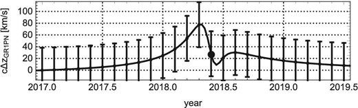
Time evolution of |$\Delta z_{\rm 1PN.0PM}(t)$| plotted with the artificial accurate data set created in step 2, for the case of GRAVITY collaboration with |$N=10$|.
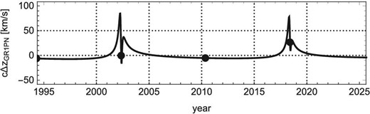
Time evolution of |$\Delta z_{\rm 1PN.0PM}(t)$| from 2000 to 2020, for the case of GRAVITY collaboration with |$N=10$|. Dots denote the pericenter and apocenter passage of S0-2 estimated by 1PN|$\, +\,$|0PM approximation. All other cases in table 2 show almost the same behavior.
3 Our observations and data analysis
Readers who want to see the results of the fitting of our observational data and the “double-peak appearance” may refer to our observational data in table 4 and go to section 4.
The observational data used in our fitting calculation are all public data released by 2017 (Boehle et al. 2016; Gillessen et al. 2017) and our spectroscopic data obtained with the Subaru telescope by 2018. We have observed S0-2 for more than 10 nights with the Subaru telescope. However, due to unfortunate bad weather conditions at the island of Hawaii in 2018, we have obtained spectra with lower SN ratios than the previous years. Our spectroscopic data, including ones reported in our previous paper (Nishiyama et al. 2018), are listed in table 4. Details on our Subaru observations are as follows.
3.1 Observation
We have carried out spectroscopic observations of S0-2 using the Subaru telescope (Iye et al. 2004) and IRCS (Kobayashi et al. 2000), in the Echelle mode. The spectral resolution of the IRCS Echelle mode is |$\approx\! 20000$| in the K band. During our observations, we have used the Subaru AO system (Hayano et al. 2008, 2010) and the laser guide star (LGS) system (Minowa et al. 2012). In the LGS mode observations, |$R = 13.8\:$|mag star USNO 0600-28577051 was used as a tip-tilt guide star, and in the natural guide star (NGS) mode, the star was used as the NGS. The details of the observations, such as exposure time and the number of frames taken in the nights, are shown in table 3. The details of the observations from 2014 to 2016 are also described in Nishiyama et al. (2018).
Summary of Subaru observations.
| Date | Setting* | IT† | |$N_{\mathrm{frame}}$| ‡ | |$N_{\mathrm{used}}$| § | Slit angle|$^{\Vert }$| | AO# |
|---|---|---|---|---|---|---|
| (UTC) | [s] | [|$^{\circ }$|] | ||||
| 2014 May 19 | |$K+$| | 300 | 32 | 30 | 8 | LGS |
| 2015 Aug 21 | |$K+$| | 300 | 24 | 24 | 8 | NGS |
| 2016 May 18–19 | |$K+$| | 300 | 48 | 44 | 8, 128 | LGS |
| 2017 May 5–8 | |$K+$| | 300 | 100 | 98 | 8, 117, 127 160, 178 | LGS |
| 2017 Aug 9–11 | |$K+$| | 300 | 68 | 57 | 8, 127 | NGS/LGS |
| 2018 March 29–30 | |$K+$| | 300 | 39 | 39 | 8, 127 | NGS/LGS |
| 2018 May 20 | |$K+$| | 300 | 34 | 32 | 68 | NGS |
| 2018 Jul 4–6 | |$K-$| | 300 | 48 | 42 | 70, 117, 160 | NGS/LGS |
| 2018 Aug 18 | |$K-$| | 300 | 24 | 24 | 8, 70 | NGS |
*IRCS Echelle setting.
†Integration time for each exposure.
‡The number of frames taken in the night(s)
§The number of frames used in data analysis.
||The angular offset measured from north to east, counterclockwise.
#The guide star of the AO system. The “LGS” mode uses the laser guide star system, and the “NGS” mode uses only a natural guide star.
3.2 Data reduction
The reduction procedure for our data sets includes:
dark subtraction;
flat-fielding;
sky subtraction;
bad pixel correction; and
cosmic ray removal.
A sky field was observed once or twice per night, and used for the correction of atmospheric emission. The S0-2 spectra are then extracted from the reduced images. The wavelength calibration was carried out using the sky OH emission lines. Spectra of nearby early-A type stars was used for the telluric correction. The details of the procedure above are described in Nishiyama et al. (2018).
3.3 Combining the S0-2 spectra
To determine the profile of the Br-|$\gamma$| absorption line and redshifts of S0-2 accurately, we have combined spectra of S0-2 from 2014 to 2017. In our previous paper (Nishiyama et al. 2018), we fitted the Br-|$\gamma$| line using a Moffat function with all parameters set as free. However, since some low signal-to-noise (SN) ratio spectra are included in our data sets, the line shape could be different in such low SN ratio spectra. Hence we have combined S0-2 spectra from 2014 May to 2017 August, to determine the profile of the Br-|$\gamma$| absorption line with a good SN ratio. Here we have not combined the spectra in 2018, because the redshift of S0-2 changes rapidly hour by hour.
To combine S0-2 spectra, first we fit the Br-|$\gamma$| line in each spectrum from 2014 to 2017 with a Moffat function, and determine the peak wavelength. The spectra are shifted to have zero redshift using IRAF dopcor task, and then combined to make a preliminary combined spectrum. Next, the Br-|$\gamma$| line in the preliminary spectrum is fitted to determine the parameter of the Moffat function. The parameters determined in this fit are used to determine the peak wavelength in each spectrum from 2014 to 2017 again. In this procedure, only the peak wavelength of a Moffat function was set to be free. The spectra are shifted to have zero redshift according to the newly determined peak wavelengths, and are then combined. Here we obtain new combined S0-2 spectrum, and fit it to determine the parameters of the Moffat function. The procedure above was repeated iteratively until any of the redshifts for individual years changes no more than |$1\:$|km|$\:$|s|$^{-1}$|.
Figure 6 shows the combined S0-2 spectra around |$2.16\, \mu$|m, using the Subaru/IRCS data sets from 2014 to 2017. The total exposure time is 21.8 hours, and the smoothing parameter of |$s = 11$|. We can find two clearly separated absorption profiles, He I |$2.16137\, \mu$|m (left) and Br-|$\gamma$||$2.16612\, \mu$|m (right). The Moffat profile used to fit the Br-|$\gamma$||$2.16612\, \mu$|m line is shown by the red curve. In the following procedure, this profile will be used to measure the peak wavelength of the Br-|$\gamma$| line. Only the peak wavelength and scaling factor (corresponding to the continuum level) are set to be free in the following profile fits.
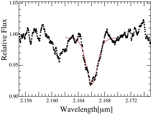
Combined S0-2 spectrum (|$s = 11$|) around the Br-|$\gamma$| absorption line, obtained with Subaru/IRCS from 2014 to 2017. We can see a He i absorption line at |$2.16137\, \mu$|m as well as the Br-|$\gamma$||$2.16612\, \mu$|m line. The Br-|$\gamma$| line is fitted with a Moffat function (red curve). (Color online)
3.4 Identification of Br-|$\gamma$| feature
The S0-2 spectra from 2014 May to 2018 August obtained with Subaru/IRCS are shown in figure 7. As shown there, the obtained spectra in 2018 are noisy. This is because of bad weather conditions, low power output of the LGS system, and frequent satellite closures during the observations in 2018. At first glance, it is not clear which feature is the Br-|$\gamma$| absorption line of S0-2. We therefore carried out an analysis to identify the Br-|$\gamma$| absorption before the fitting to determine the redshifts of S0-2.
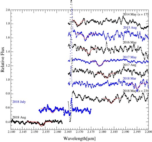
Spectra including Br-|$\gamma$| absorption line of S0-2 from 2014 May (top) to 2018 August (bottom). The fitting results are shown by red curves on the spectra. The smoothing parameters are 17 for 2014, 23 for 2018 May, and 11 for the rest of the spectra. The LSR correction is not applied. (Color online)
To identify the feature, we have used the combined spectrum of S0-2 around the Br-|$\gamma$| absorption line (figure 6). By fitting the feature, we have obtained parameters of a Moffat function which fit the feature in the combined spectrum well. Using the obtained parameters of the Moffat function for the combined spectrum, we have fitted each spectrum in 2018, by changing the central wavelength of the Moffat function. For example, in the case of the 2018 March spectra, we fitted it by changing the central wavelength of the Moffat function from 2.170 |$\mu$|m to 2.200 |$\mu$|m, and calculate |$\chi ^2$| values for the fit. When we plot |$\chi ^2$| as a function of the central wavelength, we can find a clear minimum of |$\chi ^2$| at around 2.194–|$2.195\, \mu$|m. This suggests that the absorption feature around 2.194–|$2.195\, \mu$|m is best matched with the shape of the combined spectrum, compared to other features on the 2018 March spectrum.
We have carried out the fitting described above for all the spectra obtained in 2018. We have found a clear minimum of |$\chi ^2$| at |$2.194\, \mu$|m, |$2.158\, \mu$|m, and |$2.153\, \mu$|m for the 2018 March, July, and August spectra, respectively, and thus we have considered the feature at the wavelengths as the Br-|$\gamma$| absorption line of S0-2.
For the 2018 May spectrum, we have found two minimums with similar |$\chi ^2$| values at around |$2.178\, \mu$|m and |$2.183\, \mu$|m. To identify the Br-|$\gamma$| feature, we fitted the redshifts of S0-2 using all the observed ones but that of 2018 May. The fitting result suggests that the expected redshift of S0-2 at 2018.382 (2018 May) is |${\approx} 2630\:$|km|$\:$|s|$^{-1}$|, and the central wavelength of the redshift is |${\sim}2.185\, \mu$|m. Considering the expected redshift, we have assumed that the absorption feature at around |$2.184\, \mu$|m is the Br-|$\gamma$| absorption line of S0-2 at 2018.382. Note that without such prediction from other observational results, we cannot distinguish the Br-|$\gamma$| line from other features on the 2018 May spectrum. Hence the derived uncertainty values for the 2018 May shown below are lower limits of an actual uncertainty in the redshift of S0-2.
3.5 Redshifts and uncertainties
On the S0-2 spectra from 2014 May to 2018 August (figure 7), we show the fitting results of the Br-|$\gamma$| absorption features using red curves. We use the parameters of the Moffat function determined for the combined spectrum (figure 6), but the peak wavelength and the scaling factor (corresponding to the continuum level) are left free in the fits. When we fitted the spectra, we divided the 2018 March dataset into “2018 March 29 (2018.240)” and “2018 March 30 (2018.243)” datasets. The redshifts of S0-2 are determined using the central wavelength of the fitting results, and they are shown in table 4.
Redshift and uncertainties of S0-2 in Subaru/IRCS observations.
| Time|$^\ast$| | Redshift|$_{\mathrm{LSR}}$| | |$\Delta$|redshift|$_{\mathrm{LSR}}$||$^\dagger$| | |$\sigma _{\mathrm{tot}}$| | |$\sigma _{\mathrm{JK}}$| | |$\sigma _{\mathrm{sys}}$| |
|---|---|---|---|---|---|
| [yr] | [km|$\:$|s|$^{-1}$|] | [km|$\:$|s|$^{-1}$|] | [km|$\:$|s|$^{-1}$|] | [km|$\:$|s|$^{-1}$|] | [km|$\:$|s|$^{-1}$|] |
| 2014.379 | |$\phantom{-0}485.6$| | |$+24.6$| | 26.6 | 25.6 | 6.6 |
| 2015.635 | |$\phantom{-0}886.6$| | |$-15.7$| | 16.5 | 15.5 | 5.6 |
| 2016.381 | |$\phantom{-}1096.2$| | |$+24.5$| | 16.9 | 15.2 | 7.3 |
| 2017.343 | |$\phantom{-}1768.7$| | |$+29.9$| | 20.4 | 20.0 | 5.9 |
| 2017.348 | |$\phantom{-}1798.8$| | |$+29.2$| | 14.4 | 12.9 | 6.3 |
| 2017.605 | |$\phantom{-}2133.3$| | |$-12.6$| | 27.2 | 26.1 | 7.8 |
| 2017.609 | |$\phantom{-}2169.6$| | |$-13.0$| | 36.6 | 35.7 | 8.3 |
| 2018.240 | |$\phantom{-}4001.9$| | |$+39.6$| | 36.7 | 35.4 | 9.5 |
| 2018.243 | |$\phantom{-}4096.6$| | |$+39.4$| | 39.6 | 37.7 | 12.2 |
| 2018.382 | |$\phantom{-}2466.4$| | |$+24.1$| | 67.5|$^\ddagger$| | 66.9|$^\ddagger$| | 9.1|$^\ddagger$| |
| 2018.508 | |$-1102.3$| | |$+2.2$| | 53.1 | 52.5 | 7.9 |
| 2018.628 | |$-1785.7$| | |$-15.0$| | 40.9 | 39.8 | 9.3 |
|$^\ast$|Time is counted in the unit of year, setting |$1\:$|yr as |$365.25\:$|d.
|$^\dagger$|The local standard of rest velocity at the average time of integration.
|$^\ddagger$|The shown uncertainties for 2018.382 are lower limits.
To determine the uncertainties of the S0-2 redshifts, we have conducted the same procedures described in Nishiyama et al. (2018). To estimate uncertainties, we have carried out Jackknife analysis. Before combining observed spectra, we have made N sub-data sets consisting of |$N-1$| spectra. Here N is the number of frames used in data analysis (see table 3). Then we have fitted the Br-|$\gamma$| absorption line of the N spectra of the sub-data sets, and have calculated jackknife uncertainties |$\sigma _{\mathrm{JK}}$| using equation (2) in Nishiyama et al. (2018). The obtained jackknife uncertainties are shown in table 4.
Systematic uncertainties |$\sigma _{\mathrm{sys}}$| includes the following: (1) uncertainties in spectrum smoothing (typically 1–|$2\:$|km|$\:$|s|$^{-1}$|); (2) uncertainty in the stability of the long-term wavelength calibration (|$\approx\! 5\:$|km|$\:$|s|$^{-1}$|); (3) uncertainty in the comparison of partly excluded spectra to understand the uncertainty in the telluric correction (3–|$8\:$|km|$\:$|s|$^{-1}$|). The spectra used for the fitting (figures 6 and 7) are smoothed ones, because of the faintness of S0-2. The central wavelengths could have different values when we use different smoothing parameters of the spectra. Hence we have checked how the central wavelength varies with different smoothing parameters. The typical uncertainties are estimated to be 1–|$2\:$|km|$\:$|s|$^{-1}$|.
The systematic uncertainty due to wavelength calibrations, i.e., long-term stability of this spectroscopic monitoring, is examined using the Br-|$\gamma$| “emission” line. The interstellar gas around S0-2 is ionized by UV radiation from high-mass stars nearby, and thus emits Br-|$\gamma$| which can be used to estimate the uncertainty of the wavelength calibration. Assuming the wavelength of the Br-|$\gamma$| emission line is stable from 2014 to 2018, we fit the emission line with a Gaussian function and determine the central wavelength for each spectrum. The standard deviation of the redshifts derived by the central wavelengths are |$4.9\:$|km|$\:$|s|$^{-1}$|.
One of the difficulties in data analysis of ground-based near-infrared spectroscopy is removal of telluric absorption features. In our analysis, we have observed telluric standard stars and used them to remove the telluric lines. However, the strength and profile of the telluric lines vary with atmospheric conditions and airmass of targets. Hence we have examined the change of the central wavelengths of the Br-|$\gamma$| absorption line by using sub-sets of spectra, part of which is excluded from the original spectra (for more detail, see Nishiyama et al. 2018). In this experiment, we have examined how the central wavelength changes if a part of the Br-|$\gamma$| absorption feature is affected by uncorrected telluric absorption. The uncertainties derived by the fits of the partly excluded spectra are 3–|$8\:$|km|$\:$|s|$^{-1}$| from 2014 to 2018, and these uncertainties are also quadratically added to the final systematic uncertainties of |$\sigma _{\mathrm{sys}}$| (table 4).
Note that, as described in subsection 3.4, it is difficult to identify the Br-|$\gamma$| absorption feature in the 2018 May spectrum without a prediction from other data sets. Hence the uncertainties derived for 2018.382 (table 4) are likely to be underestimated compared to actual ones.
4 Time evolution of |$\Delta z_{\rm 1PN.0PM}(t)$| fitted with observational data
As derived in section 2, the difference between the GR and Newtonian redshifts under our presupposition |$\Delta z_{\rm 1PN.0PM}(t)$| shows the “double-peak appearance” in its time evolution. In this section, we examine whether the double-peak appearance is found or not in the observational data, including our 2018 data.
Note that the observational data used in our analysis include not only our own data but also all public data released by the other groups by 2017, while the VLT group (GRAVITY collaboration 2018) did not use the astrometric data of the Keck group (Do et al. 2019), and the Keck group did not use the astrometric data of the VLT group. Further, the new 2018 data in GRAVITY collaboration (2018) and Do et al. (2019) are not used in our analysis, because those data were not available for us when this paper was written.
4.1 Parameters determined by our fitting
The parameters determined by the |$\chi ^2$|-fitting in the following discussions are not only the 11 parameters listed in sub-subsection 2.4.1 but also the parameters corresponding to the origin of the astrometric data of Keck and VLT groups. Their astrometric origins are set at the position of an infrared flare near Sgr A|$^\ast$| at a certain time. The flare position at a certain time may be moving relative to Sgr A|$^\ast$| (and to our astrometric center “C” introduced in appendix 1). Therefore, the vector |$\boldsymbol {A}_{\rm sky}(t)$| defined in equation (A3) of appendix 1 does not vanish for either Keck or VLT astrometric data. Then, we introduce the following eight parameters corresponding to |$\boldsymbol {A}_{\rm sky}(t)$|:
|$\Delta {\rm RA}_{\rm K.apo}$|: the RA of the astrometric origin |$\boldsymbol {A}_{\rm apo}$| at the apocenter time |$t_{\rm S.apo}$| for the Keck data.
|$\Delta {\rm DEC}_{\rm K.apo}$|: the Dec of the astrometric origin |$\boldsymbol {A}_{\rm apo}$| at the apocenter time |$t_{\rm S.apo}$| for the Keck data.
|$V_{\rm K.ra}$|: the RA-component of the velocity of astrometric origin |$\boldsymbol {V}_{\rm astro}$| for the Keck data.
|$V_{\rm K.dec}$|: the Dec-component of the velocity of astrometric origin |$\boldsymbol {V}_{\rm astro}$| for the Keck data.
|$\Delta {\rm RA}_{\rm V.apo}$|: the RA of the astrometric origin |$\boldsymbol {A}_{\rm apo}$| at the apocenter time |$t_{\rm S.apo}$| for the VLT data.
|$\Delta {\rm DEC}_{\rm V.apo}$|: the Dec of the astrometric origin |$\boldsymbol {A}_{\rm apo}$| at the apocenter time |$t_{\rm S.apo}$| for the VLT data.
|$V_{\rm V.ra}$|: the RA-component of the velocity of astrometric origin |$\boldsymbol {V}_{\rm astro}$| for the VLT data.
|$V_{\rm V.dec}$|: the Dec-component of the velocity of astrometric origin |$\boldsymbol {V}_{\rm astro}$| for the VLT data.
In total, we determine the 19 parameters by |$\chi ^2$|-fitting of the S0-2 motion with real astrometric and spectroscopic observational data.
4.2 Results of fitting
As the first step, we perform three |$\chi ^2$|-fittings in order to obtain three sets of parameter values :
Fitting 1 (“GR-best-fit”): We perform the |$\chi ^2$|-fitting of the real observational data with the S0-2 motion at the 1PN|$\, +\,$|0PM approximation. Then we obtain the GR best-fitting values of the 19 parameters, which are shown in table 5. With these parameter values, the redshift at the 1PN|$\, +\,$|0PM approximation, |$cz_{\rm 1PN.0PM}(t)$|, is calculated using equation (11).
Fitting 2 (“NG-best-fit”): We perform the |$\chi ^2$|-fitting of the real observational data with the S0-2 motion in the Newtonian gravity. Then we obtain the NG best-fitting values of the 19 parameters, which are shown in table 5. With these parameter values, the redshift in the Newtonian gravity, |$cz_{\rm NG}^{\rm (real)}(t)$|, is calculated using equation (3). Here the upper suffix “(real)” denotes that this Newtonian redshift is obtained from the real observational data.
Fitting 3 (“NG-art-best-fit”): We create the ideally accurate, artificial data set using the GR-best-fit values of the 11 parameters listed in sub-subsection 2.4.1, where we set |$N=20$| and |$L=64\:$|yr, which are the parameters introduced in sub-subsection 2.4.2.8 Then, we perform the |$\chi ^2$|-fitting of this artificial data set with the S0-2 motion in the Newtonian gravity, and we obtain the NG artificial best-fitting values of the 11 parameters, which are shown in table 5. With these parameter values, the redshift in the Newtonian gravity, |$cz_{\rm NG}^{\rm (art)}(t)$|, is calculated using equation (3). Here the upper suffix “(art)” denotes that this Newtonian redshift is obtained from the artificial data set.
Results of our |$\chi ^2$|-fitting.|$^*$|
| |$\chi _{\rm red.min}^2$| and parameters | |$\chi _{\rm red.min}^2$| | |$M_{\rm SgrA}$| | |$R_{\rm GC}$| | |$V_{\rm O.ra}$| |
|---|---|---|---|---|
| determined by |$\chi ^2$|-fitting | [no dim.] | [|$10^6\, M_\odot$|] | [kpc] | [mas|$\:$|yr|$^{-1}$|] |
| GR-best-fit | 1.1903 | |$4.232\pm 0.066$| | |$8.098\pm 0.066$| | |$-0.162\pm 28.782$| |
| NG-best-fit | 1.2134 | |$4.274\pm 0.067$| | |$8.114\pm 0.067$| | |$-0.168\pm 29.056$| |
| NG-art-best-fit | 0.0754 | |$4.352\pm 0.020$| | |$8.207\pm 0.018$| | |$-0.128\pm 0.002$| |
| Parameters | |$V_{\rm O.dec}$| | |$V_{\rm O.Z}$| | |$I_{\rm S}$| | |$\Omega _{\rm S}$| |
| [mas|$\:$|yr|$^{-1}$|] | [km|$\:$|s|$^{-1}$|] | [|$^{\circ }$|] | [|$^{\circ }$|] | |
| GR-best-fit | |$0.174\pm 28.787$| | |$-8.345\pm 3.213$| | |$134.239\pm 0.217$| | |$227.766\pm 0.242$| |
| NG-best-fit | |$0.166\pm 29.061$| | |$5.261\pm 3.196$| | |$134.063\pm 0.214$| | |$227.518\pm 0.245$| |
| NG-art-best-fit | |$0.191\pm 0.001$| | |$9.307\pm 1.070$| | |$134.306\pm 0.056$| | |$226.974\pm 0.066$| |
| Parameters | |$\omega _{\rm S}$| | |$e_{\rm S}$| | |$T_{\rm S}$| | |$t_{\rm S.apo}$| |
| [|$^{\circ }$|] | [no dim.] | [yr] | [AD] | |
| GR-best-fit | |$66.204\pm 0.333$| | |$0.8903\pm 0.0007$| | |$16.0504\pm 0.0023$| | |$2010.3383\pm 0.0015$| |
| NG-best-fit | |$66.049\pm 0.340$| | |$0.8911\pm 0.0007$| | |$16.0468\pm 0.0022$| | |$2010.3432\pm 0.0014$| |
| NG-art-best-fit | |$65.521\pm 0.062$| | |$0.8899\pm 0.0002$| | |$16.0489\pm 0.0003$| | |$2010.3410\pm 0.0003$| |
| Parameters | |$\Delta {\rm RA}_{\rm K.apo}$| | |$\Delta {\rm DEC}_{\rm K.apo}$| | |$V_{\rm K.ra}$| | |$V_{\rm K.dec}$| |
| [mas] | [mas] | [mas|$\:$|yr|$^{-1}$|] | [mas|$\:$|yr|$^{-1}$|] | |
| GR-best-fit | |$0.576\pm 0.611$| | |$-1.796\pm 0.611$| | |$0.262\pm 28.790$| | |$-0.708\pm 28.790$| |
| NG-best-fit | |$0.689\pm 0.620$| | |$-1.725\pm 0.620$| | |$0.309\pm 29.063$| | |$-0.692\pm 29.063$| |
| Parameters | |$\Delta {\rm RA}_{\rm V.apo}$| | |$\Delta {\rm DEC}_{\rm V.apo}$| | |$V_{\rm V.ra}$| | |$V_{\rm V.dec}$| |
| [mas] | [mas] | [mas|$\:$|yr|$^{-1}$|] | [mas|$\:$|yr|$^{-1}$|] | |
| GR-best-fit | |$-1.061\pm 0.611$| | |$2.152\pm 0.611$| | |$0.154\pm 28.790$| | |$-0.220\pm 28.790$| |
| NG-best-fit | |$-0.964\pm 0.620$| | |$2.223\pm 0.620$| | |$0.200\pm 29.063$| | |$-0.199\pm 29.063$| |
*GR-best-fit is the result of fitting the real observational data with the S0-2 motion at the 1PN|$\, +\,$|0PM approximation of GR. NG-best-fit is the result of fitting the real observational data with the S0-2 motion in the Newtonian gravity. NG-art-best-fit is the result of fitting the artificial accurate data with the S0-2 motion in the Newtonian gravity, where the artificial data are created from the GR-best-fit. The error in |$\chi ^2$|-fitting is given by definition (18).
Figure 8 shows the GR evidence represented by our fitting results listed in table 5. The first and second panels focus around the recent pericenter passage, where the solid curve is the time evolution of the observed GR evidence |$c\Delta z_{\rm 1PN.0PM}^{\rm (observe)}(t)$| and the dashed curve is the theoretically expected time evolution of the GR evidence |$c\Delta z_{\rm 1PN.0PM}^{\rm (expect)}(t)$|. The third and fourth panels focus around the previous pericenter passage. The fifth panel shows the whole temporal range covering all real observational data, in which the Subaru data are denoted by blue, the Keck data by red, and the VLT data by green. Those data points are |$c\Delta z_{\rm obs}$|, defined in equation (15).
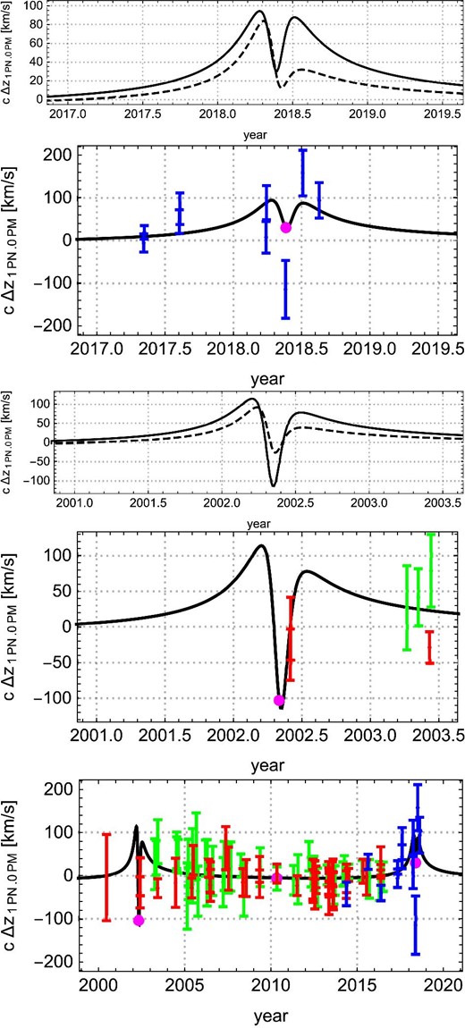
GR evidence described by our fitting results. In all panels, the solid curve is the real GR evidence, |$c\Delta z_{\rm 1PN.0PM}^{\rm (real)}(t)$|, obtained from the real observational data, and the dashed curve is the theoretically expected GR evidence, |$c\Delta z_{\rm 1PN.0PM}^{\rm (art)}(t)$|. The blue data are of Subaru observations, red data of Keck, and green data of VLT, where all data are subtracted by the Newtonian best-fitting redshift |$cz_{\rm NG}^{\rm (real)}(t)$|. Magenta dots denote the pericenter and apocenter passages. The first and second panels focus around the recent pericenter passage. The third and fourth panels focus around the previous pericenter passage. The fifth panel shows the temporal range including all real observational data. (Color online)
The double-peak appearance around the recent and previous pericenter passages are recognized in the observed GR evidence (solid curve in figure 8). In order for a quantitative assessment of the detection of the GR evidence under our presupposition on the parameter values, we need a quantity that can measure the discrepancy/similarity between the solid curve and the dashed curve in figure 8. Such a quantity is defined in subsection 4.3.
Here we summarize some points found in figures 9 and 10. Figure 9 shows the “previously used” GR evidence (the special relativistic and gravitational Doppler components in |$\Delta z_{\rm 1PN.0PM}$|) given by the formula (19), which corresponds to the case of |$f=1$| of |$\Delta z_{\rm GR}^{\rm (prev)}$| in equation (17). We find that our largest magnitude of the previously used GR evidence |${\approx} 200\:$|km|$\:$|s|$^{-1}$| appears around the pericenter passage (|$2018.3850\:$|yr in 1PN|$\, +\,$|0PM motion of S0-2). This is consistent with the results of the other groups.
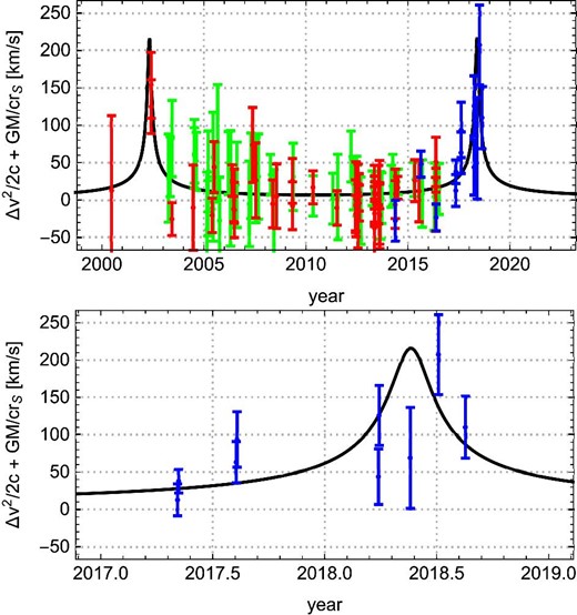
Previously used GR evidence given by equation (19) with GR-best-fit parameters. The top panel shows the temporal range for all observational data. The bottom panel focuses around the recent pericenter passage. The blue data are of Subaru observations, red data of Keck, and green data of VLT, where all data are subtracted by the LSV part of GR redshift (first and second terms of equation (11)). (Color online)
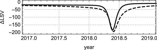
Difference of LSV between 1PN|$\, +\,$|0PM (GR-best-fit) and Newtonian cases. For the solid curve, the Newtonian case is given by the NG-best-fit parameters. For the dashed curve, the Newtonian case is given by the NG-art-best-fit parameters, corresponding to the bottom panel of figure 3.
Note that the largest magnitude of |$\Delta z_{\rm 1PN.0PM} \approx\! 100\:$|km|$\:$|s|$^{-1}$| under our presupposition (see figure 8) is about a half of that of the previously used GR evidence |${\approx} 200\:$|km|$\:$|s|$^{-1}$|. Even when the previously used GR evidence would be detected with a given observational data set, the significance for the detection of |$\Delta z_{\rm 1PN.0PM}$| would be smaller under our presupposition.
Figure 10 shows the difference of the LSV between the 1PN|$\, +\,$|0PM motion of S0-2 (GR-best-fit parameters) and the Newtonian motion of S0-2 (NG-best-fit or NG-art-best-fit), given by equation (20). For the solid curve, the Newtonian motion is given by the NG-best-fit parameters. For the dashed curve, the Newtonian motion is the NG-art-best-fit parameters (corresponding to the bottom panel of figure 3). The negativity of both solid and dashed curves denotes that the Newtonian LSV is faster than the GR LSV in both NG-best-fit and NG-art-best-fit. Further, from figures 9 and 10, it is recognized that the summation of the previously used GR evidence and the LSV difference results in the double-peak appearance of our GR evidence |$\Delta z_{\rm 1PN.0PM}(t)$| shown in figure 8. This is consistent with the simulation (figure 3) performed in sub-subsection 2.4.4.
4.3 A quantity to measure the discrepancy between the GR and the Newtonian gravity
The denominator of |$\delta z(t_0,\delta t)$| represents an absolute amount of the theoretically expected GR evidence |$\Delta z_{\rm 1PN.0PM}^{\rm (expect)}(t)$| for duration |$\delta t$| from |$t_0$|. For example, in the first panel of figure 8, the denominator corresponds to the area between the horizontal axis and the curve of |$c \Delta z_{\rm 1PN.0PM}^{\rm (expect)}(t)$| (dashed curve).
The numerator of |$\delta z(t_0,\delta t)$| represents an absolute amount of the difference between the observed GR evidence |$\Delta z_{\rm 1PN.0PM}^{\rm (observe)}$| and the theoretically expected one |$\Delta z_{\rm 1PN.0PM}^{\rm (expect)}$| for duration |$\delta t$| from |$t_0$|. For example, in the first panel of figure 8, the numerator corresponds to the area between the curve of |$c \Delta z_{\rm 1PN.0PM}^{\rm (observe)}(t)$| (solid curve) and the curve of |$c \Delta z_{\rm 1PN.0PM}^{\rm (expect)}(t)$| (dashed curve). Note the mathematical fact that, if the real observational data expresses exactly the theoretically expected time evolution of the GR evidence under our presupposition, then the numerator of |$\delta z$| must be zero.
The quantity |$\delta z(t_0,\delta t)$| defined in equation (23) is the ratio of the “difference between |$\Delta z_{\rm 1PN.0PM}^{\rm (observe)}$| and |$\Delta z_{\rm 1PN.0PM}^{\rm (expect)}$|” to the “amount of |$\Delta z_{\rm 1PN.0PM}^{\rm (expect)}$|”, for duration |$\delta t$| from |$t_0$|. In other words, this |$\delta z$| expresses to what extent the GR evidence in the real observational data matches well with the theoretically expected GR evidence under our presupposition on the parameter values.
We propose this |$\delta z(t_0,\delta t)$| as a measure of the discrepancy/similarity between the GR and the Newtonian gravity under our presupposition on the parameter values.
To calculate the value of |$\delta z(t_0,\delta t)$|, we need to determine not only the values of |$t_0$| and |$\delta t$| but also the three sets of parameters GR-best-fit, NG-best-fit, and NG-art-best-fit. Using the three sets of best-fitting parameters listed in table 5, some values of |$\delta z(t_0,\delta t)$| for some combinations of |$(t_0,\delta t)$| are listed in table 6. This table implies that the present real observational data include about |$60\%$| error in measuring the double-peak appearance of the GR evidence. In order to reduce this error and to confirm the detection of the double-peak appearance, we need additional data sets.
Error, |$\delta z(t_0,\delta t)$|, that estimates a discrepancy between the observed GR evidence |$\Delta z_{\rm 1PN.0PM}^{\rm (observe)}$| and the theoretically expected GR evidence |$\Delta z_{\rm 1PN.0PM}^{\rm (expect)}$| for the real observational data set.
| |$\delta z(t_0,\delta t)$| | Counted from |$t_0$| [yr] | With duration |$\delta t$| [yr] |
|---|---|---|
| 0.651 | 2000.475* | 18.135† |
| 0.603 | |$2018.628-T_{\rm S}$| |$^\ddagger$| | |$T_{\rm S}$| |
| 0.623 | |$t_{\rm S.apo}$| | |$T_{\rm S}$| |
| 0.636 | 2000.475 | |$T_{\rm S}$| |
| 0.620 | |$t_{\rm S.apo}-T_{\rm S}$| § | |$T_{\rm S}$| |
| 0.584 | |$t_{\rm S.apo}-\frac{T_{\rm S}}{2}$| || | |$T_{\rm S}$| |
*The first spectroscopic data was observed at 2000.475 by Keck, and the latest data was at 2018.628 by Subaru shown in table 4.
†Temporal range of the real spectroscopic data is |$\delta t = 2018.628-2000.475 = 18.135\:$|yr.
‡ |$T_{\rm S}$| and |$t_{\rm S.apo}$| are in the GR-best-fit parameters in table 5, that correspond to, respectively, the recent apocenter time in 2010 and the period of the S0-2 motion.
§ |$t_{\rm S.apo}-T_{\rm S}$| is about the time at previous apocenter in 1994.
|| |$t_{\rm S.apo}-T_{\rm S}/2$| is about the time at previous pericenter in 2002.
5 Summary and discussion
Under the presupposition on the parameter values given in section 1, we have proposed a theoretical discussion on the GR evidence that appears in the spectroscopic data of the S0-2 motion. The GR evidence under our presupposition, |$\Delta z_{\rm 1PN.0PM}(t)$| defined in equation (14), is the difference between the GR and Newtonian redshifts of photons coming from S0-2. In section 2, under our presupposition, we have revealed that the theoretically expected time evolution of |$\Delta z_{\rm 1PN.0PM}(t)$| shows two peaks, before and after the pericenter passage of S0-2. This “double-peak appearance” is a significant feature which expresses the discrepancy between GR and Newtonian gravity under our presupposition on the parameter values. (The double peaks reduce to a single peak under the treatment of the parameter values by other groups, as summarized in subsection 2.3.) It has also been found that the |$\chi ^2$|-assessment under the present averaged observational uncertainties is not useful to confirm the detection of the double-peak appearance.
In section 3, our observations with the Subaru telescope by 2018 have been summarized. Due to unfortunate bad weather conditions at Hawaii island in 2018, our data in 2018 have lower SN ratio than the previous years. In section 4, it has been shown that the double-peak appearance can be recognized in the present observational data (figure 8). However, as shown in figure 8, the uncertainties of our 2018 data are so large that we cannot exclude the Newtonian case (|$z_{\rm obs} \equiv z_{\rm NG}$|). Further, according to the quantity |$\delta z$| which measures the discrepancy between the GR and the Newtonian gravity under our presupposition on the parameter values, the error in measuring the double-peak appearance in the present data set is about 60%. In order to reduce this error and to confirm the detection of the double-peak appearance, we need additional data sets.
Finally, let us discuss one method for the test of GR or the so-called modified theories of gravity, under our presupposition on the parameter values. Note again that the quantity |$\delta z$| estimates the discrepancy between the GR and the Newtonian gravity under our presupposition. Therefore, if we replace the GR with a modified theory of gravity in the definition of |$\delta z$|, then the modified |$\delta z$| can be interpreted as a measure of the discrepancy between the modified theory of gravity and the Newtonian gravity. Hence, if the value of |$\delta z$| of the GR is lower than the value of |$\delta z$| of the other theories of gravity, then it is reasonable to conclude that the GR is more promising than the other theories of gravity.
Acknowledgments
We would like to express our gratitude to the staffs of the Subaru telescope, for their continuous supports for our observations. We thank Rainer Schödel for his supports in our data analysis, and Aurelien Hees for his useful discussions on the theory for detecting the GR evidence. H. S. was supported by JSPS KAKENHI, Grant-in-Aid for Challenging Exploratory Research 26610050, and Grant-in-Aid for Scientific Research (B) 19H01900. S. N. was supported by JSPS KAKENHI, Grant-in-Aid for Young Scientists (A) 25707012, Grant-in-Aid for Challenging Exploratory Research 15K13463 and 18K18760, and Grant-in-Aid for Scientific Research (A) 19H00695. T. O. was supported by JSPS KAKENHI, Grant-in-Aid for JSPS fellows JP17J00547. Y. T. was supported by JSPS KAKENHI, Grant-in-Aid for Young Scientists (B) 26800150. M. T. was supported by DAIKO FOUNDATION, and JSPS KAKENHI, Grant-in-Aid for Scientific Research (C) 17K05439.
Appendix 1. Set-up of our coordinate system
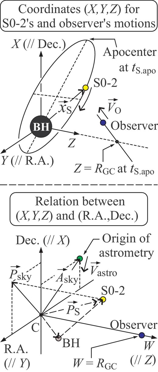
The top panel denotes the coordinate system |$(X,Y,Z)$| for calculating the motions of S0-2 and observer. The origin of |$(X,Y,Z)$| is fixed at Sgr A|$^\ast$|, and the origin of time is set at the apocenter time of S0-2, |$t_{\rm S.apo}$|. The bottom panel shows the relation between |$(X,Y,Z)$| and the astrometric coordinate system, right ascension (RA) and declination (Dec). The center “C” of RA and Dec is at distance |$R_{\rm GC}$| in the direction parallel to Z-axis, and the origin of astrometric observations is, in general, moving relative to C. (Color online)
Finally, we make two comments. First, because the center C at the apocenter time |$t_{\rm S.apo}$| is just at Sgr A|$^\ast$| [the origin of coordinates |$(X,Y,Z)$|], the first term |$\boldsymbol {A}_{\rm apo}$| in equation (A3) is also the position of astrometric origin measured from Sgr A|$^\ast$| at |$t_{\rm S.apo}$|. Secondly, because the velocities |$\boldsymbol {V}_{\rm astro}$| and |$\boldsymbol {V}_{\rm O}$| are, respectively, measured from C and Sgr A|$^\ast$|, the relative velocity of the astrometric origin measured from Sgr A|$^\ast$| is given by |$\boldsymbol {V}_{\rm astro}+\boldsymbol {V}_{XY}$|, where |$\boldsymbol {V}_{XY}$| is the projection of |$\boldsymbol {V}_{\rm O}$| on to the X-Y plane.
Appendix 2. Derivation of |$z_{\rm 1PN.0PM}(t)$| and some analyses of |$\Delta z_{\rm 1PN.0PM}(t)$|
A.2.1 Derivation of the GR redshift (11)
This appendix is for the derivation of the GR redshift of photons coming from S0-2 at the 1PN|$\, +\,$|0PM approximation (11). This redshift can be obtained by substituting the definition of frequency (5) into the definition of redshift (1) under the 1PN|$\, +\,$|0PM approximation.
By the definition of LNRF, the time-like vector |$e_{(t)}^\mu$| has no angular velocity with respect to the spacelike hypersurface at |$t=$| constant. However, this vector has a non-zero |$\varphi$|-component, |$e_{\rm (t)}^\varphi \ne 0$|, in the Boyer–Lindquist coordinates. The angular velocity of |$e_{(t)}^\mu$| measured in the Boyer–Lindquist coordinates (not in a coordinate system fixed to the hypersurface at |$t=$| constant), |$e_{(t)}^{\varphi }/e_{(t)}^t = \omega (r,\theta )$|, is regarded as the angular velocity of the so-called “frame dragging effect” of a Kerr BH measured in the Boyer–Lindquist coordinates. However, as shown below, the frame dragging effect cannot be detected within the observational precision of current telescopes (which corresponds to the 1PN and 0PM approximations of GR).
A.2.2 Some analyses of the GR evidence (14)
In comparing the GR prediction with the Newtonian prediction, one may consider that the Newtonian time |$t_{\rm NG}$| corresponds to the proper time of S0-2, |$t_{\rm NG} \leftrightarrow \tau$|, or to the Lorentz-transformed case, |$t_{\rm NG} \leftrightarrow \tau /\sqrt{1-(V_{\rm S}/c)^2}$|. However, the difference between these correspondences of the temporal coordinates do not affect the following discussions at the 1PN|$\, +\,$|0PM approximation. Note that the latter correspondence is estimated as |$t_{\rm NG} \leftrightarrow \tau /\sqrt{1-(V_{\rm S}/c)^2} \approx\! (1 + \varepsilon ) \tau$|, where the order relation |$V_{\rm S}/c \sim O(\varepsilon ^{1/2})$| is used. The term |$\varepsilon \tau$| can be absorbed into the second term in equation (A34). Therefore, the latter correspondence degenerates to the former one, |$t_{\rm NG} \leftrightarrow \tau$|, at the 1PN|$\, +\,$|0PM approximation. This correspondence of the temporal coordinates is assumed in the following discussions.
Footnotes
From the results of the Planck satellite observations in 2018 (Planck Collaboration 2018), a modified gravitational theory, such as the Starobinsky model, may be considered as a good candidate theory of gravity under some assumptions. However, such discussions are for the early/inflationary universe and seems not to be applicable to the Galactic center scale. Therefore, we assume GR that is to be compared with Newtonian gravity at the Galactic center. A comment on the modified theories of gravity will be given at the end of section 5.
We use the term “line-of-sight” velocity instead of “radial” velocity, in order to avoid the confusion with the “radial” component |$V^r$| of the velocity |$\boldsymbol {V}$| defined in our coordinate system |$(r,\theta ,\varphi)$| centered at Sgr A|$^\ast$|.
In the Newtonian case, one may not include the Roemer time delay because the light speed is treated as infinity in the Newtonian dynamics. However, in this paper, we give priority to the fact that the light speed is finite, and introduce the Roemer time delay not only in the GR case but also in the Newtonian case.
In the previous papers, in addition to the assessment of GR hypothesis, a direct comparison of the GR and Newtonian best-fitting orbits of S0-2 has been discussed through the Bayesian approach (e.g., using the so-called Bayes factor or Occam factor), or the so-called reduced-chi-squared |$\chi _{\rm red}^2$| with putting higher weights on the data in 2018 than the other data.
We are interested in the physical property of |$\Delta z_{\rm GR}$|, which appears in the time evolution within a period |$\approx\! T_{\rm S}$|. Hence, we make the ideally accurate data set cover at least one period of the S0-2 motion.
Note that the |$\chi ^2$|-assessment for discriminating some theories and the |$\chi ^2$|-fitting for searching the best-fitting parameter values of each theory are different. In this paragraph we discuss only on the |$\chi ^2$|-assessment.
The gravitational potential of BH estimated in GR is stronger than the one in Newtonian gravity. This makes the speed of S0-2 in the GR case tend to be greater than the speed in the Newtonian case, and the pericenter time in the GR case precedes the pericenter time in the Newtonian case.
The values of |$N=20$| and |$L=64\:$|yr are one example. The other cases satisfying the conditions given in sub-subsection 2.4.2 result in the same conclusion with this section.
References
