


Abstract
Hinode is Japan’s third solar mission following Hinotori (1981–1982) and Yohkoh (1991–2001): it was launched on 2006 September 22 and is in operation currently. Hinode carries three instruments: the Solar Optical Telescope, the X-Ray Telescope, and the EUV Imaging Spectrometer. These instruments were built under international collaboration with the National Aeronautics and Space Administration and the UK Science and Technology Facilities Council, and its operation has been contributed to by the European Space Agency and the Norwegian Space Center. After describing the satellite operations and giving a performance evaluation of the three instruments, reviews are presented on major scientific discoveries by Hinode in the first eleven years (one solar cycle long) of its operation. This review article concludes with future prospects for solar physics research based on the achievements of Hinode.
Table of contents
1. Introduction … … … … … … … … … … … … 3
T. Watanabe
2. Mission operation and instrument performance . . 5
2.1. Mission operation … … … … … … … … … … 5
T. Shimizu
2.2. Solar Optical Telescope (SOT) … … … … … … 6
Y. Suematsu & T. D. Tarbell
2.3. X-ray Telescope (XRT) … … … … … … … … . 10
T. Sakao
2.4. EUV Imaging Spectrometer (EIS) … … … … … . 13
K. Al-Janabi, D. Baker, L. Bradley, D. H. Brooks, J. L. Culhane, G. Del Zanna, G. Doschek, H. Hara, L. Harra, S. Imada, J. Mariska, I. Ugarte-Urra, H. P. Warren, T. Watanabe, & P. Young
3. Quiet Sun … … … … … … … … … … … … … 15
3.1. Quiet-Sun magnetism: Flux tubes, horizontal fields, and intra-network fields … … … … … . . 15
L. R. Bellot Rubio
3.2. The quiet-Sun magnetism and the solar cycle … . 23
R. Centeno
3.3. Spicules … … … … … … … … … … … … … . 26
T. M. D. Pereira
4. Polar region activities … … … … … … … … … . 29
4.1. Magnetic patches in polar regions … … … … . . 29
D. Shiota
4.2. Coronal activities in polar regions … … … … . . 31
M. Shimojo
5. Prominences: Structures and flows … … … … … 33
5.1. Active region vs. quiescent prominence structuring and dynamics … … … … … … … . 33
A. S. Hillier
5.2. Prominence thermal and velocity structure as seen with EIS and XRT … … … … … …35
A. S. Hillier
5.3. Prominence plumes and the magnetic Rayleigh–Taylor instability … … … … … … . . 36
A. S. Hillier
5.4. MHD turbulence in prominences … … … … … 37
A. S. Hillier
5.5. Coronal rain … … … … … … … … … … … . . 37
P. Antolin & A. S. Hillier
5.6. Summarizing prominence dynamics with Hinode 38
A. S. Hillier
6. Heating of the upper atmosphere … … … … … . 39
6.1. Observational signatures of chromospheric and coronal heating by transverse MHD waves … . . 39
P. Antolin
6.2. Nanoflare heating: Observations and theory … . . 47
J. A. Klimchuk
7. Active regions … … … … … … … … … … … . . 50
7.1. Sunspot structure … … … … … … … … … … . 50
S. K. Tiwari
7.2. Coronal jets … … … … … … … … … … … … 59
A. C. Sterling
7.3. Emerging flux … … … … … … … … … … … . 63
S. Toriumi
7.4. Active region loops … … … … … … … … … . . 69
H. P. Warren
8. Flares and coronal mass ejections … … … … … . 77
8.1. Flare energy build-up: Theory and observations. 77
Y. Su
8.2. Flare observations: Energy release and emission from flares … … … … … … … … … … … … 82
L. Fletcher
8.3. Initiation of CMEs … … … … … … … … … . . 88
K. K. Reeves
9. Slow solar wind and active-region outflow … … . 93
D. H. Brooks
10. Future prospects … … … … … … … … … … … 96
S. K. Solanki
Acknowledgments … … … … … … … … … … ….101
Appendix. List of abbreviations … … … … … … … .101
References … … … … … … … … … … … … … … .102
Overall arrangements by T. Sakurai
1 Introduction
The Institute of Space and Astronautical Science, Japan Aerospace Exploration Agency (ISAS/JAXA), successfully launched the M-V Launch Vehicle No. 7 (M-V-7) with SOLAR-B aboard at 6:36 am on 2006 September 23 JST (21:36 UTC on September 22) from the Uchinoura Space Center (USC): the spacecraft was nicknamed “Hinode,” meaning “sunrise” in Japanese.
This is the third Japanese solar physics mission following Hinotori (ASTRO-A; Kondo 1982) and Yohkoh (SOLAR-A; Ogawara et al. 1991). The spinning satellite Hinotori was launched in 1981, and aimed to observe high-energy aspects of solar activity in X-rays and γ-rays. The scientific impact of the X-ray observations from Hinotori on solar flare research was thoroughly reviewed by Tanaka (1987). Superhot components seen in hydrogen-like iron emission lines were first discovered by the onboard flat crystal spectrometers (Tanaka 1986), and Hinotori proposed three types (A, B, and C) for flare classification through its morphological and spectral observations in X-rays.
The Yohkoh satellite was three-axis stabilized, and it was launched on 1991 August 30. The mission continued scientific operations for more than a decade until the spacecraft lost its attitude control during the annular eclipse on 2001 December 14. The Yohkoh mission found various kinds of magnetic structures and active phenomena emerging in the solar corona, and confirmed that solar flares were powered by magnetic reconnection (Uchida et al. 1996). Hard X-ray sources were detected “above the loop-top region” to identify the reconnection region, which is also the site for particle acceleration in solar flares (Masuda et al. 1994). In soft X-rays the flaring loops often present the shape of cusps, the structure that the standard models expect in the process of magnetic reconnection taking place high in the solar corona (Tsuneta 1996). Sheared coronal loops followed by ejection of plasma clouds and sudden coronal dimming during solar flares (Sterling et al. 2000), X-ray jets (Shimojo et al. 1996), and tiny microflares in active regions (Shimizu 1995) have all been recognized as manifestations of magnetic reconnection, and dynamical evolutions of these phenomena were observed for the first time by the Soft X-ray Telescope (SXT) experiment on Yohkoh (Tsuneta et al. 1991), which registered more than one million whole-Sun X-ray images, and they were finally combined into 3 × 10⁵ composite images in order to increase the dynamic range of each image by carefully calibrating the on-orbit performance of the spacecraft (Acton 2016).
Based on these discoveries of its predecessors, the Hinode mission (Kosugi et al. 2007) was designed to address the fundamental question of how magnetic fields interact with the ionized atmosphere to produce solar variability. The major scientific goals of the Hinode mission are: (a) understanding the processes of magnetic field generation and transport, including magnetic modulation of solar luminosity; (b) investigation of the processes responsible for energy transfer from the photosphere to the corona and for heating and structuring the chromosphere and the corona; and (c) identification of the mechanism responsible for eruptive phenomena, such as flares and coronal mass ejections (CMEs) in the context of the space weather of the Sun–Earth system.
The Hinode satellite (figure 1) contains three instruments dedicated to observing the Sun: the Solar Optical Telescope (SOT), the X-Ray Telescope (XRT), and the EUV Imaging Spectrometer (EIS). These instruments were developed by ISAS/JAXA in cooperation with the National Astronomical Observatory of Japan (NAOJ) as domestic partner, and the National Aeronautics and Space Administration (NASA; US) and the Science and Technology Facilities Council (STFC; UK) as international partners. The European Space Agency (ESA) and Norwegian Space Center (NSC) provide downlink stations (Sakurai 2008). The spacecraft completed its major initial operations including orbit adjustment to a Sun-synchronous orbit and performance verification of the attitude control system in early 2006 October.
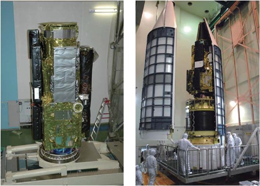
Hinode spacecraft. On the left-hand-side panel, we can see EIS to the left and XRT to the right of the satellite body. At its center is SOT, with the focal-plane package (FPP) on our side. (Color online)
All the data taken by Hinode have been open to the public since the successful completion of the commissioning phase in 2007 May. This open data policy was approved and adopted by the Hinode Science Working Group (SWG), the top-level science steering group that is attended by the principal investigators (PIs) and the project managers (PMs) representing each space agency. It was founded in 2003 to discuss all the issues involved in enhancing the scientific outputs from the Hinode mission. The SWG encourages simultaneous and collaborative observations with other solar observation satellites and ground-based facilities, and especially coordination among the three instruments on board Hinode.
The Hinode SWG also recommends holding science meetings regularly. The tenth-anniversary science meeting of the Hinode launch was held at Sakata and Hirata Hall in Nagoya University on 2016 September 5–8. More than 160 solar physicists attended this meeting from 14 countries. Taking advantage of the above opportunity, this review paper has been completed as a joint work among the invited speakers to the meeting for each science topic, as well as PMs and instrument PIs, to assess the Hinode scientific achievements thoroughly during the first decade since its launch.
Throughout this article, the following non-SI units and their abbreviations are used: gauss (G), hectogauss (hG), kilogauss (kG), maxwell (Mx). MK means 106 K. One arcsec on the solar surface seen from the Earth at 1 au corresponds to 726 km. The Appendix contains a list of abbreviations used in this article for instrument names and so on.
2 Mission operation and instrument performance
2.1 Mission operation
The Hinode satellite (Kosugi et al. 2007), launched on 2006 September 22 (UTC), went through orbit maintenance maneuvers, and was finally installed into a circular, sun-synchronous polar orbit of about 685 km altitude and |${98{^{\circ}_{.}}1}$| inclination. This orbit has provided continuous solar viewing conditions for a duration of nine months each year, with an eclipse season from early May to early August in which a night period with a longest duration of 20 min exists every 98 min orbital period. This sun-synchronous condition is expected to be maintained until at least 2020 without any orbit maneuvers.
The spacecraft system functions and their performance are healthy, excepting for an anomaly in the X-band mission data downlink channel. Starting at the end of 2007, the onboard X-band modulator began to produce irregular signals in the latter half of each contact with the ground stations. The frequency of the occurrence increased with time, and finally the X-band downlink function became unavailable. After 2008 March, the mission data downlink path was switched to the S-band backup path. Since the bandwidth of the S-band path (262 kbps) is about 16 times lower than that of the X-band path (4 Mbps), we have increased the number of downlink passes by adding many ground stations to the Hinode downlink network, with strong support from the space agencies. Since 2009 we have typically gained 43–54 downlink passes per day, providing about 7–10 hr as the total downlink duration per day. By efficiently utilizing the data volume available from scheduled downlink passes, although limited to 15%–20% of the data volume in the X-band era (40–50 Gbits), the observation planning of each telescope has been carried out with best-tuned observing parameters, including the field of view (FOV), the number of wavelengths observed, pixel summation, and image compression, for meeting the scientific objectives of each observation. The cadence of observations may be reduced to fit the telemetry resource. Data-demanding observations, such as high-cadence and highest spatial resolution observations, may be restricted to a minimum required duration with reduced FOV sizes and number of observables. The 24 hr continuous observations may be given up by inserting idle periods of observations when data-demanding observations are scheduled. The available data volume is shared among the three instruments with a typical ratio of SOT:XRT:EIS = 70%:15%:15%, which can be changed depending on observations.
High spatial resolution is one of the important scientific accomplishments achieved by Hinode. The spacecraft is stabilized by the attitude and orbit control system (AOCS) in three axes with its Z-axis pointed to the Sun. The AOCS primarily uses four momentum wheels as the actuators, with signals of sub-arcsec accuracy from two fine sun sensors (Ultra-Fine Sun Sensor; UFSS) for the solar direction, an inertial reference unit comprising four gyros for detecting temporal changes of attitude with very high accuracy, and a star tracker for determining the roll of the spacecraft. The spacecraft jitter is measured to be 0|${^{\prime\prime}_{.}}$|1–0|${^{\prime\prime}_{.}}$|2 (σ) in 10 s, and 0|${^{\prime\prime}_{.}}$|3 (σ) in 60 s in magnitude, which is sufficient for XRT and EIS observations. A much higher stability of the SOT images is achieved by an image stabilization system (see sub-subsection 2.2.1). It is noted that the spin speed of the momentum wheels, which should be controlled around ±1800 rpm, shows a gradual drift and the high-frequency micro-vibration excited by the wheels may give fairly large jitter of the order of |${0{^{\prime \prime }_{.}}3}$| (|$3\, \sigma$|) to the SOT images when the speed becomes around 2200 rpm. To avoid such degraded performance, the reset operation of the momentum wheels’ speed has been carried out every 3–4 yr. The co-alignment among the telescopes with the orbital period behavior of the telescope pointing has been monitored by performing a co-alignment program run repeatedly during the mission (Shimizu et al. 2007; Minesugi et al. 2013).
The mission operations, i.e., daily commanding and telemetry checking, have been conducted from Sagamihara Spacecraft Operation Center (SSOC) in ISAS. The SSOC is in real-time contact with the Hinode spacecraft in limited periods from Monday through Saturday via antennas at Uchinoura and in the JAXA Ground Network. The planning of the three telescope operations is coordinated by a Chief Planner (CP), whose duties include scheduling the spacecraft pointing and merging instrument commands into an integrated spacecraft load. Telescope science operations are carried out by Chief Observers (COs). Each CO is responsible for developing the observation sequence for the telescope and coordinating this plan with other telescope plans as well as with the scientists requesting the observations. The CO activities are performed with the participation of scientists and graduate students from cooperating institutes and universities in Japan as well as from the institutes and universities involved in the instrument development in the US, UK, and Norway. All the CO activities were performed at SSOC for a few years after the launch, but remote planning from his/her home institute was introduced for the COs’ activities.
In addition to the observation plans led by each instrument team (core programs), the Hinode team has accepted observation proposals from many researchers from around the world.1 The Science Schedule Coordinators (SSC) group reviews the proposals in monthly meetings, gives their advice to proposers for better observations, approves the acceptance of proposals, and schedules the accepted proposals as Hinode Operation Plans (HOPs).2 The observation planning, such as the spacecraft pointing (observing target) schedule, is coordinated among the three telescopes by discussions among the COs and CP in the daily meeting (10:30 JST on Monday–Saturday) and the weekly meeting (after the daily meeting on Friday). The final adjustment of the spacecraft pointing is made in the daily meeting before the command uplink in the evening. In the X-band era, the planning was conducted in one-day intervals for Monday–Friday uploads and two days for Saturday upload. After switching to the S-band downlinks, the interval was increased for better planning of observations by effectively utilizing the volume of the onboard data recorder; the timelines are uploaded on Tuesday, Thursday, and Saturday. To reduce the operational cost, Focused Mode operations, in which only one timeline upload is scheduled in a week, have been introduced for three to four months per year, after some trials in 2014. Hinode observations are currently coordinated extensively with IRIS. At the appearance of an active region expected to show large flares, the operation team may postpone or discontinue the scheduled HOP observations and switch to flare watch observations as soon as possible.
Any data acquired by the core programs and HOPs are fully open to any users immediately after the reformatted data are provided via the data centers.3 No priority is given to HOP proposers in data usage. All the Hinode-related science and operations activities have been supervised by the international steering committee, i.e., the SWG.
2.2 Solar Optical Telescope (SOT)
The Solar Optical Telescope has an aperture of 0.5 m and achieves a diffraction-limited angular resolution of 0|${^{\prime\prime}_{.}}$|2–0|${^{\prime\prime}_{.}}$|3 in the 380–660 nm range. It was optimized for accurate measurement of vector magnetic fields in the photosphere and dynamics of both the photosphere and chromosphere associated with the magnetic fields—see the overview by Tsuneta et al. (2008b). SOT consists of two optically separable components: the Optical Telescope Assembly (OTA), consisting of a 0.5 m aperture aplanatic Gregorian-type telescope with a collimating lens unit, a polarization modulation unit (PMU), and an active tip–tilt mirror (Suematsu et al. 2008b); and an accompanying Focal Plane Package (FPP), housing two filtergraphs (FG)—a narrow-band (NFI) and a broad-band (BFI) filtergraphic imager—and a spectro-polarimeter (SP) at a pair of photospheric magnetic sensitive lines of Fe i 630.15/630.25 nm (Lites et al. 2013).
The PMU at the exit pupil of the OTA modulates the polarization state of the incoming beam for the measurement of magnetic field vectors by a continuously rotating waveplate with a revolution period of 1.6 s. The temperature dependence of the retardation is minimized by utilizing two crystals (quartz and sapphire) of compensating thermal coefficients of birefringence. All optical elements prior to the PMU are rotationally symmetric about the optical axis in order to minimize instrumental polarization.
SOT observations are carried out under very stable conditions (stability requirement <0|${^{\prime\prime}_{.}}$|09 in 3 σ) achieved by a combination of the satellite attitude control system, structural design, and active image stabilization. The image stabilization system consists of a piezo-driven tip–tilt mirror (CTM) in the OTA in a closed-loop servo using the displacement error estimated from correlation tracking of solar granulation (correlation tracker; CT). This system minimizes jitter in solar images on the focal plane CCDs (Shimizu et al. 2008b).
The FPP is configured with a reimaging lens followed by the beam splitter for the filtergraph, the spectro-polarimeter, and the correlation tracker channels. The FPP performs both filter (FG) and spectral (SP) observations at high polarimetric precision, and both types of observation can be performed simultaneously but independently. In filter observation, a 4k × 2k CCD camera is shared by the BFI and the NFI, which are selected by a common mechanical shutter. The SP and CT have their own CCD detectors. This complex instrument allows very accurate magnetic field measurements in both longitudinal (along the line of sight) and transverse directions under precise polarimetric calibration (Ichimoto et al. 2008c), Doppler shift measurements, and imaging in the range from the low photosphere through the chromosphere.
The sequence control of the SOT observations is managed by the observation tables in the Mission Data Processor (MDP; Matsuzaki et al. 2007). Separate observation tables were prepared for FG observation and for SP observation. The table contains several lists of commands for acquiring observables on a time interval schedule. Commands for taking observables are issued according to these tables, and the FPP takes action in response to them.
The contents of the tables are composed from pre-arranged science observing plans and are uploaded from the ground station. Science data are acquired by the FG and SP CCD cameras. Multiple images can be exposed to derive observables such as Dopplergrams and magnetograms. In these cases, exposed data are processed in the FPP in real time to reduce the amount of data. For example, in the case of the SP, spectra are exposed and read out continuously 16 times per rotation of the polarization modulator, and the raw spectra are added and subtracted on board in real time to be demodulated, generating Stokes I, Q, U, and V spectral images. The processed science data are then transferred to the MDP via a high-speed parallel interface. Because of the limited telemetry downlink bandwidth, data are compressed in pixel depth (16 to 12 bit compression) as well as in two-dimensional image planes (image compression). The MDP re-forms the compressed data into CCSDS (Consultative Committee for Space Data Systems) packets and sends them to the Data Handling Unit (DHU) for recording in the Data Recorder (DR).
The MDP has eight kinds of lookup tables to perform the 16 to 12 bit compression with different compression curves. For image compression of SOT data, two algorithms are available for different compression parameter tables: one is 12 bit JPEG DCT (discrete cosine transform) lossy compression and the other is 12 bit DPCM (differential pulse code modulation) lossless compression. Typically, filtergram data can be compressed to 3 bits pixel−1 by the JPEG algorithm and Stokes vector data to 1.5 bits pixel−1 when the noise due to lossy compression is comparable to the photon noise level in the data, although the compression ratio is highly dependent upon the nature of the images.
2.2.1 On-orbit performance
The on-orbit performance of SOT has generally proved to be excellent and met or exceeded all prelaunch requirements for the BFI, SP, and CT. However, it turned out soon after the first-light observation that images from the NFI contained the blemishes that degraded or obscured the image over part of the FOV. These were caused by air bubbles in an index-matching oil inside the tunable birefringent (Lyot) filter. In the following, some key aspects of on-orbit performance of SOT are given.
Optical performance
The image stabilization is critical for high-resolution and high-precision polarimetric observations. It was evaluated by the displacement of an image taken by the CT camera at 580 Hz with respect to a reference image fixed for ∼40 s. While the CT servo is on, the image stability gets as high as 0|${^{\prime\prime}_{.}}$|01 root mean square (rms) in both X and Y directions (X in solar east–west, Y in north–south directions), which is about three times smaller than the requirement. It was confirmed that moving mechanisms in the three telescopes of Hinode do not produce a significant degradation of the SOT images during their movement except for the visible-light shutter (VLS) of XRT, which produces an SOT image jitter of about 0|${^{\prime\prime}_{.}}$|4 rms during the period of its movement (∼0.5 s). However, the influence of the XRT VLS on the SOT observation is negligibly small since the frequency of its usage is sufficiently low.
The BFI produces photometric images with broad spectral coverage in six bands [CN band (388.3 nm), Ca ii H line (366.8 nm), G band (430.5 nm), and three continuum bands (450.4 nm, 555.0 nm, 668.4 nm)] at the highest spatial resolution available from SOT (0|${^{\prime\prime}_{.}}$|0541 per pixel sampling) and at a rapid cadence (<10 s typical, minimum 1.6 s for a smaller FOV) over a 218|${^{\prime \prime }}$| × 109|${^{\prime \prime }}$| FOV. Exposure times are typically 0.03–0.8 s, but longer exposures are possible. The BFI is capable of accurate measurements of proper motion and temperature in the photosphere, and of high-resolution imaging of some structures in the chromosphere, and measurements in the three shortest wavelength bands permit identification of sites of kilogauss-strength magnetic field outside sunspots.
Diffraction-limited optical performance of the BFI was confirmed using a point-like structure seen in G-band images. The size of the point-like structure is fairly close to that from a theoretical point spread function (PSF) for the observing wavelength (Suematsu et al. 2008b). The PSFs for all BFI wavelengths were also measured by Mathew, Zakharov, and Solanki (2009) using Mercury transit data of 2006 November (see also Wedemeyer-Böhm 2008). The dark disk-like Mercury images were convolved with a model PSF, generated by a combination of four two-dimensional Gaussians, to fit the observed intensity profiles. The narrowest Gaussian in all cases closely reproduces the theoretical angular resolution of the OTA, while the remaining Gaussians with much broader widths mainly account for the scattered light in the OTA.
In the case of the SP, the intensity contrast of granulations observed by the SP was compared with those from three-dimensional (3D) radiative magnetohydrodynamic (MHD) simulations to estimate its PSF (Danilovic et al. 2008). It was confirmed that the observed contrast is reproduced well by the convolution of the synthetic image from the MHD simulation with a PSF derived from the shape of the OTA entrance pupil having a slight defocus aberration in which the Strehl ratio is close to 0.8.
As expected, a gradual change in the best focus position was observed, which is mainly caused by dehydration shrinkage in space of the CFRP (carbon-fiber-reinforced plastics) truss pipes connecting the primary with the secondary mirror of the OTA. However, it unexpectedly turned out that the focus also changes according to the change in pointing on the solar disk; however, the focus offset is about seven steps in reimaging lens displacement (0.17 mm step−1) from disk-center to limb pointing. Although the cause of this focus change is not well understood, the response is fast enough to allow us to readjust the reimaging lens position at each maneuver of the satellite during operation. During the eclipse season (from early May to early August), a large focus drift (∼12 steps) occurs ∼30 min from the dawn in each orbit. This is a predicted behavior caused by thermal deformation by the day/night cycle of the heat-dump-mirror cylinder and its supporting spider which can displace the secondary mirror. The eclipse season is certainly a degraded performance period for SOT. The gradual focus drift almost ended after 2011 when the dehydration of the CFRP slowed down and the temperature of the OTA became stable by heater control, although the short-term focus change due to pointing change still remains and is corrected during operation.
The BFI has a chromatic aberration which was unexpectedly recognized after the launch. Then, it was noticed that a relay lens of the BFI had been flipped from the original optical design in the ground test to have co-focus with NFI and SP, which works in air but not in vacuum. The focus difference between 388 nm and 668 nm is about nine steps (= 1.53 mm of the reimaging lens displacement). If the reimaging lens is set at the center of the chromatic aberration, the focus offset is about four steps at the longest or shortest wavelength, and the corresponding wave-front error is 21 nm rms. Thus the impact of the chromatic aberration is small, but not negligible when we observe in two extreme wavelengths simultaneously. There is no evidence of chromatic aberration in the NFI, and the SP is well co-focused with the BFI 668 nm (Ichimoto et al. 2008b).
It was confirmed in an early commissioning phase that the light levels in individual observing wavelengths were close to those predicted from the ground Sun tests. It turned out, however, that the throughputs of all observing wavelengths have decreased monotonically in such a manner that those of shorter wavelengths have steeper degradation. At the beginning of 2011, the throughput became about 32% at 388.3 nm, 40% at 396.8 nm, 62% at 430.2 nm, 77% in the blue continuum, and 87%–89% in the green and red continua. The throughputs at the two shorter wavelengths have recovered since then up to 50%–55% and become stable, while those at longer wavelengths keep decreasing. The SP (630.2 nm) throughput has become 64% in the ten years since first light; accordingly, the signal-to-noise ratio has gone down to 80%. The causes of the degradation and recovery are not identified, although contaminants accumulating on the OTA optics and cleaning by atomic oxygen in the phase of high solar activity might be possibilities. The baking of the FG CCD did not help in recovering the throughput.
Spectro-polarimeter
The SP is designed to be operated flexibly in mapping observing regions, allowing one to perform suitable observations depending on science objectives. It has a number of modes of operation: Normal Map, Fast Map, Dynamics, and Deep Magnetogram. The Normal Map mode produces polarimetric accuracy in the polarization continuum of about 0.0012 Ic with 4.8 s integration and the spatial sampling of 0|${^{\prime\prime}_{.}}$|16 × 0|${^{\prime\prime}_{.}}$|16 (Lites et al. 2008). It takes 83 min to scan a 160″-wide area, large enough to cover a moderate-sized active region. By reducing the scanning size, the cadence becomes faster (50 s for mapping a 1|${^{\prime\prime}_{.}}$|6-wide area). The Fast Map mode, which is mostly used to save telemetry, provides 30 min cadence for 160″-wide scanning with polarimetric accuracy of 0.1% but a 0|${^{\prime\prime}_{.}}$|32 sampling. The Dynamics mode provides higher cadence (18 s for a 1|${^{\prime\prime}_{.}}$|6-wide area) with a 0|${^{\prime\prime}_{.}}$|16 sampling, although at lower polarimetric accuracy.
In Deep Magnetogram mode, photons can be accumulated over many rotations of the polarization modulator, as long as the data do not overflow the CCD summing registers. This allows one to achieve a very high degree of polarization accuracy in very quiet regions, at the expense of time resolution. Using this mode for data of an effective integration time of 67.2 s, the rms noise in the polarization continuum of the spectra was estimated to be about 3 × 10⁻⁴, corresponding to |$1 \, \sigma$| noise levels of 0.6 G and 20.1 G for the longitudinal and transverse components of magnetic flux density, respectively (Lites et al. 2008).
The SP shows an orbital drift of the spectral image on the CCD with an amplitude of about 10 pixels (p–p) in both directions along and perpendicular to the slit. The cause is displacement of the Littrow mirror due to thermal deformation of the FPP structure according to the orbital motion. The drift rate was minimized by optimizing the temperature settings of the operational heaters attached to the FPP structure, and is finally corrected by the calibration software SP_PREP (Lites & Ichimoto 2013).
Narrow-band Filtergraphic Imager
The NFI provides intensity, Doppler, and full Stokes polarimetric imaging at high spatial resolution (0|${^{\prime\prime}_{.}}$|08 per pixel sampling) in any one of ten spectral lines [including the Fe lines (525.0 nm, 557.6 nm, 630.2 nm), having a range of sensitivity to the Zeeman effect, Mg i b2 (517.3 nm), Na D1 (89.6 nm), and Hα] over the full FOV (328|${^{\prime \prime }}$| × 164|${^{\prime \prime }}$|). The spectral lines span the photosphere to the lower chromosphere for diagnosis of dynamical behavior of magnetic and velocity fields at the lower atmosphere. The passband of the Lyot filter is 9 pm and the wavelength center is tunable to several positions in a spectral line and its nearby continuum. It is noted that the edges of the full FOV are slightly vignetted due to the limited size of the optical elements of the Lyot filter residing in a telecentric beam. The unvignetted area is 264|${^{\prime \prime }}$| in diameter. Exposure times are typically 0.1–1.6 s, but longer exposures are possible.
Shutterless modes with the frame transfer operation of the CCD are used for higher time resolution (1.6–4.8 s) and polarimetric sensitivity, although the FOV is restricted by a focal plane mask. With a 0.1 s exposure, 16 images are taken in a revolution of the PMU waveplate. These images are successively added or subtracted in the four slots of the smart memory to create the Stokes IQUV images. The modulation frequency is two per PMU rotation for V and four per PMU rotation for Q and U.
Images of the NFI contained blemishes due to bubbles in the oil of the Lyot filter which degraded or obscured the image over part of the FOV. They distorted and moved when the Lyot filter was tuned. For this reason, NFI usually ran in one spectral line at one or a small number of wavelengths for a sequence of observations. Rapid switching between spectral lines was inhibited in its operation. To suppress the disturbance by the bubbles, it was required to block four tuning elements out of eight. This situation limited the capability of tuning the filter, but some useful schemes were still available. New software to enable such operations was successfully uploaded twice, in 2007 April and September, and tuning schemes have been developed and tested which permit tuning to different positions in a line profile without disturbing the bubbles. Thus, 50%–75% of the FOV remained usable in most NFI observations.
Doppler and magnetogram observations using two wavelengths remained possible. However, multi-wavelength scans of Stokes parameters, for vector field inversion, had become generally impossible. Wavelength scans in Hα were also severely curtailed because of the bubble motion they caused. These limitations interfered with some science goals regarding rapid evolution of vector magnetic fields and chromospheric structure and dynamics in active regions, flares, and prominences.
It was also found that the transmission of the blocking filters was degrading rapidly. The cause was identified as filter coating damage due to solar UV flux. Five of the six blocking filters have zinc sulfide coating layers which absorb UV light below ∼420 nm and change its index of refraction. As a result, the transmission profiles shifted to the blue and were badly distorted (Title 1974). The Fe i 630.2 nm filter was severely damaged and quickly became unusable; about 60% of throughput was lost in a year from first light. Since only the blocking filter for Na i D1 589 nm is durable against the UV, this filter is always inserted in the beam during the idle time, to slow the degradation of other filters. Thus, the magnetograms and Dopplergrams in the Na i D1 line were used in most NFI observations.
In 2010 the filter bubbles disappeared, either dissolving back into the oil or moving out of view. For about two years, NFI observations with multiple lines and wavelength settings were possible using the whole FOV, though with limitations on the usage of the vulnerable blocking filters. Early in 2013 a bubble reappeared at a location where it did not move with tuning but caused image degradation over part of the field. Users of NFI data from this period should contact the SOT team if they have questions about the image quality of specific datasets. Many observing programs used offsets from the center of the FOV to put the target in an area with uncompromised image quality.
2.2.2 Conclusions and future observing
The Solar Optical Telescope is the largest state-of-art optical telescope yet flown in space to observe the Sun. It has exhibited excellent performance on-orbit for more than eleven years. Many excellent papers have been published to date as given elsewhere in this review paper using SOT’s unprecedentedly high-quality data for the sub-photosphere (local helioseismology) through the chromosphere.
Although ground-based telescopes make observations of the same type and at the same wavelengths as the SOT, the telescope in space derives great advantages from the uniformity of its observing conditions: (1) high resolution at all times over all of its FOV, (2) continuous temporal coverage, and (3) unprecedented polarimetric sensitivity at small spatial scales. Discovery of waves on spicules and prominence threads, bubbles and instabilities in prominences, and penumbral microjets are examples of the first advantage. Continuous, multi-day studies of the emergence and evolution of network and intra-network magnetic flux are enabled by the second. All three advantages contribute to the spectro-polarimetric contributions to understanding both global and local dynamos, with cycle-long observations of the polar fields and of the weak, quiet Sun fields at all latitudes.
Magnetic fields transport energy into the upper atmosphere through emerging fields, propagating waves, and work done on existing magnetic footpoints by photospheric motions. Free energy can be stored in magnetic fields, which is dissipated via magnetic reconnection and induces MHD instability and eruptions. Therefore, to understand the origin of solar active phenomena, it is very important to measure the underlying magnetic fields accurately, with high spatial resolution and good temporal coverage of their resolution.
Higher temporal, spatial, and velocity resolution than what previous satellites provided has allowed us to measure waves in the atmosphere in a way we were unable to do before. Previous attempts to detect MHD waves using ground-based observations have yielded ambiguous results, but SOT has opened the door to these waves being observed in many different circumstances; the waves may carry enough energy to heat the corona and accelerate the solar wind in the quiet Sun.
The SOT observations of active regions provided some evidence that an average vertical Poynting flux, in which photospheric motion shuffles the footpoints of coronal magnetic fields, varied spatially, but was upward and sufficient to explain coronal heating.
High-resolution SOT observations also revealed that magnetic reconnection similar to that in the corona is occurring at a much smaller spatial scale throughout the chromosphere, and suggested that heating of the solar chromosphere and corona may be related to small-scale ubiquitous magnetic reconnections. This finding promotes further study of magnetic reconnection in the atmosphere, where atoms are only partially ionized and collisional, in contrast to the coronal conditions.
Unfortunately, SOT FG observation was terminated at the end of 2016 February, because of short circuit trouble in the FG camera’s electronics. However, the SP is still healthy and performing various observations, focusing on higher resolution and a wider FOV. It should be stressed that the quality of SP polarization data is even superior in contrast to ground-based 1 m-class telescopes. New inversion techniques for deriving the magnetic field from spectro-polarimetric data are being advanced greatly by the application of spatial deconvolution techniques (e.g., Buehler et al. 2015; Quintero Noda et al. 2015) to enhance small-scale magnetic structure. Furthermore, the combination of SP with IRIS and ground-based advanced chromospheric (magnetic field) observations can provide a 3D view of magnetic structure, and we can expect more accurate quantitative analysis of evolving small-scale magnetic structure and the associated Poynting flux across the photosphere.
2.3 X-ray Telescope (XRT)
2.3.1 Overview
The X-Ray Telescope for Hinode (Golub et al. 2007; Kano et al. 2008) employs Wolter I-like grazing-incidence optics (Wolter 1952; van Speybroeck & Chase 1972) to observe the Sun’s corona with broad-band temperature response. The telescope was built to achieve the highest-ever angular resolution (2″ at the best focus position) among grazing-incidence X-ray imagers for the Sun while maintaining a wide FOV that can cover the whole Sun.
While the Soft X-ray Telescope (SXT) aboard Yohkoh (Tsuneta et al. 1991) was sensitive to coronal plasmas with temperatures typically above 3 MK, XRT was designed to extend its temperature coverage down to ≲1 MK by employing a back-illuminated CCD [sensitive to both soft X-ray and extreme ultraviolet (EUV) wavelengths, and also to visible light] as the focal-plane detector. The extended wavelength coverage of XRT, up to 200 Å, has enabled the telescope to observe not only soft X-rays but also EUV emissions from warm (≲1 MK) plasmas in the corona. Similarly to Yohkoh/SXT, XRT employs a set of two filter wheels placed in front of the CCD. Each of the filter wheels has multiple X-ray analysis filters with which the temperatures of a wide range of coronal plasmas from below 1 MK up to beyond 20 MK can be derived using ratios of X-ray signals from a pair of analysis filters (Hara et al. 1994; Acton et al. 1999). The temperature diagnostic capability of XRT with such a “filter-ratio method” is summarized in Narukage et al. (2011, 2014).
In addition to the X-ray optics, the telescope employs visible-light optics with a lens located at the Sun-facing end of the telescope. The visible-light telescope has two G-band (430 nm) filters (an entrance aperture filter and a focal-plane filter) to produce a high-contrast photospheric image on the CCD. These G-band visible-light images are used for co-aligning X-ray images with images from other telescopes (including those taken on the ground), utilizing photospheric features such as sunspots and the visible solar limb.
XRT was built, and has been operated, under close international collaboration between the U.S. and Japan. The Smithsonian Astrophysical Observatory (SAO), under a contract from NASA, provided the telescope (X-ray mirror and the metering tube), filter wheels, focus adjustment mechanism for the CCD, and the electronics for driving the filter wheels and sending exposure trigger signals to the CCD. JAXA and NAOJ developed the focal-plane CCD camera which contains the focus stage on which the CCD is mounted, and the camera electronics. The CCD camera was mated to the telescope at SAO. The entire XRT then went through a series of environmental (mechanical and thermal) tests at NASA/Goddard Space Flight Center (GSFC) followed by successful completion of X-ray focusing performance tests at NASA/Marshall Space Flight Center (MSFC). After the tests in the U.S., XRT was shipped to ISAS/JAXA and was integrated into the spacecraft for the final system tests.
Onboard observation with XRT is made through the MDP, which contains observation tables with which exposure commands are successively sent to XRT at time intervals given in the currently running observation table—see Kano et al. (2008) for details. Like the other telescopes aboard Hinode, XRT has been operating remarkably well for the past eleven years since launch, providing various discoveries in the field of solar physics as described in the subsequent sections of this article. In the following, some key aspects of the on-orbit instrumental performance of XRT are reported.
2.3.2 On-orbit instrumental performance
Focusing performance
The optics of XRT gives a plate scale such that a single pixel of the focal-plane CCD (13.5|$\, \mu$|m size) corresponds to an angular scale of 1″ (Golub et al. 2007). The on-orbit performance of the X-ray optics (the angular resolution, the off-axis scattering performance, and the plate scale) of XRT has been studied by several authors using XRT observation of the transit of Mercury in front of the Sun (Shimizu et al. 2007; Weber et al. 2007), through image co-alignment studies (Yoshimura & McKenzie 2015), and using XRT images of the Venus transit (Afshari et al. 2016). To the best of our knowledge, the XRT optics has been stably providing superior X-ray imaging performance that is fully consistent with prelaunch measurements. Discussion of the effect of vignetting of the XRT mirror, together with comprehensive characterization of the image signal outputs from the CCD, is given by Kobelski et al. (2014b).
In general, the Wolter I optics exhibits some image curvature around the focal point—see, e.g., figure 3 of Golub et al. (2007). This, in turn, implies that one can have high-spatial-resolution images with a relatively narrow FOV in an image plane placed at around the best on-axis focus position while modest-resolution images with a wide FOV in another image plane placed ahead (nearer to the Sun) of the best focus position. By moving the focus stage along the optical axis, XRT adopts two CCD positions; one is referred to as the “Narrow Field Focus” and the other as the “Wide Field Focus.” The former puts the imaging surface of the CCD 81|$\, \mu$|m ahead of the best on-axis focus position determined by the preflight focusing performance tests. This gives an rms blur diameter of less than 1″ for an off-axis angle up to >8′. The Narrow Field Focus position is used for most XRT images that are taken with a limited FOV. The Wide Field Focus, for which the CCD is placed 251|$\, \mu$|m ahead of the best on-axis focus position, is typically used for synoptic full-Sun images, which have been regularly taken twice a day (usually at around 6 UT and 18 UT of each day) to observe, e.g., long-term variations of the corona in multiple X-ray analysis filters. This focus position provides images with less than 2″ rms blur diameter for an extended off-axis angle up to ∼15′. The absolute focus position is calibrated once every week by referring to a built-in mechanical reference in the focus adjustment mechanism.
Temperature diagnostics with X-ray analysis filters
Precise calibration of X-ray analysis filters is key for deriving correct filter-ratio temperatures with XRT. In addition to prelaunch calibration of the filters with X-rays as reported in Golub et al. (2007), the thicknesses of all the X-ray analysis filters were further calibrated using on-orbit data by Narukage et al. (2011). The focal-plane CCD and the analysis filters have been suffering from molecular contamination which deteriorates the sensitivity of the XRT, in particular at longer X-ray wavelengths. On-orbit calibration was performed together with characterizing the possible chemical composition of the contamination material and its time-dependent accumulation thickness onto the CCD and each of the analysis filters. Such characterization of the molecular contamination is detailed in Narukage et al. (2011). In order to minimize permanent accumulation of the contaminants on the CCD, XRT conducts a regular CCD decontamination bake-out once every three weeks. Each bake-out lasts for three days, during which the CCD temperature is kept between +30°C and +35°C. The interval and the duration of the CCD bake-out have been determined to minimize the impact on observations while removing most, if not all, contaminants accumulated on the CCD.
The calibration of the filter thicknesses made in Narukage et al. (2011) was based chiefly on quiet-Sun data due to the low solar activity during the period in which the calibration was made. This has left some room for further refinement of the filter thicknesses for thicker filters that are used for observing hot plasmas in active regions and in flares. An update to the calibration using active region data was made in Narukage et al. (2014) which improved the characterizing thicknesses of the thicker filters.
Image co-alignment
Precise knowledge of the position of each XRT image with respect to the solar disk is indispensable for co-aligning XRT data with images from other telescopes/facilities. Effort to establish co-alignment between images from multiple instruments including XRT was initiated soon after launch (the first one being the co-alignment effort between SOT and XRT; Shimizu et al. 2007) and is still ongoing. Extensive characterization of XRT co-alignment features utilizing Hinode’s UFSS (Tsuno et al. 2008) and the 335 Å band of the Atmospheric Imager Assembly onboard the Solar Dynamics Observatory (SDO/AIA; Lemen et al. 2012) was conducted by Yoshimura and McKenzie (2015). Their work has enabled co-aligning XRT images with an accuracy much better than 1″.
Some part of the entrance filter of XRT was broken on orbit: first on 2012 May 9 and secondly on 2015 June 14, with two additional small breaks in 2017 May and 2018 May. Note that a similar break in the entrance filters was also experienced by Yohkoh/SXT, whose visible-light contamination of X-ray images was carefully studied and characterized by Acton (2016). The increased level of visible-light contamination through the X-ray optics path forced a shortening of exposure durations for taking G-band images; they can still be taken without saturation in the CCD output, but it turned out that the shortest exposure time (1 ms) had to be adopted after the second break. In addition to the increased G-band intensity on the CCD, stray-light features also appeared in G-band images. These features can be removed by taking a G-band image with the shutter (VLS) closed and subtracting that image from the corresponding image taken with the VLS open. As well as the impact on visible-light exposures, the break in the entrance filters has also introduced visible light into X-ray images taken with some of the analysis filters that are not opaque enough to visible light. The filters with discernible visible-light contamination (C-poly, Ti-poly, and Al-mesh filters) are currently either no longer used for regular observations (C-poly and Ti-poly; they can be substituted by other filters in terms of temperature coverage) or used with stray-light correction (Al-mesh) when faint features are studied with that filter. Careful calibration of the stray light in X-ray images after the first break in the entrance filter was reported in Takeda, Yoshimura, and Saar (2016). Calibration of the visible-light contamination after the second entrance filter break is also under way.
Flare detection
One of the key features of Hinode in observing flares is that it utilizes XRT images for detecting the occurrence of a flare (Kano et al. 2008). XRT takes the so-called “flare patrol images” with the entire image area of the CCD, interrupting the ongoing regular observations, at a certain interval (currently every 30 s unless the exposure interval of regular observations is longer than that). The series of flare patrol images are then analyzed by the MDP, which identifies the occurrence of a flare as an increase in X-ray intensity of a certain region of the corona imaged by XRT. Upon detection of a flare, the MDP switches the observation sequence of XRT to the one for flares (by switching the active observation table to the one for flares) and, at the same time, informs the occurrence of a flare to SOT and EIS together with its positional information.
As XRT acts as the flare monitor for the entire Hinode mission, it is crucially important to detect flares efficiently from the beginning. A requirement was set such that major flares whose peak GOES (Geostationary Operational Environmental Satellite) X-ray flux reaches at least a middle-M class shall be detected when the X-ray flux reaches 1/10 of the peak flux, and the flare detection parameters (such as the time interval for taking flare patrol images and the threshold for the increase in X-ray intensity) were tuned accordingly. The tuning was made with multiple series of actual flare patrol images and a software simulator with the flare detection logic of the MDP. The resultant flare detection performance with XRT is discussed in Sakao (2018), showing a satisfactory outcome.
2.3.3 Typical observation sequences
In regular observations, XRT takes synoptic images of the full-Sun X-ray corona in multiple X-ray filters (e.g., with the Al-poly, Al-mesh, and Be-thin filters) twice a day: one at around 6 UT and the other around 18 UT, each lasting for about 10 min. For each of the X-ray filters, a set of images are taken with short and long (or short, medium, and long) exposures to generate composite images avoiding saturation of the CCD output for bright active regions while properly imaging faint X-ray structures of the non-bright regions of the corona. The synoptic images are processed, archived, and released at the website4 so that the images can be utilized for studying long-term changes of the X-ray corona. Figure 2 depicts some examples of XRT synoptic images with the Al-poly filter, each made as a composite of multiple exposure times. In addition to these synoptic observations, XRT also performs synoptic full-Sun exposures with an increased number of X-ray filters (typically with about six different filter combinations) twice a week to increase the variety of synoptic images.
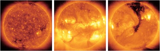
Some examples of synoptic images taken with the Al-poly filter of XRT on 2008 July 22 (left), 2012 September 28 (middle), and 2016 March 25 (right). Each image is made as a composite of multiple exposure times, avoiding saturation of signal outputs across the image area of the focal-plane CCD. The left-hand panel corresponds to the minimum phase of the solar activity cycle, while the middle one is near the maximum phase of the activity, and the right-hand one in the declining phase of the activity. (Color online)
For periods other than the daily synoptic observations, XRT carries out a variety of observations depending on the HOPs of the day, or on the observation plan discussed and agreed among the COs of the three scientific instruments who are in charge of the observation planning for the relevant day. The non-synoptic, regular observations typically consist of observing the target on the Sun with a limited FOV (by reading out limited image areas on the CCD such as 512 × 512 or 384 × 384 pixel areas out of the entire image area of 2048 × 2048 pixels) to increase the exposure cadence by reducing the data volume of the images taken. These images are taken with the Narrow Field Focus position (see sub-subsection 2.3.2, Focusing performance).
When a flare is detected by the MDP, XRT starts to observe the flare by performing a sequence of exposures defined in the MDP flare-observing table. With the flare-observing table, XRT takes images of the flare with relatively thick analysis filters (such as the Be-thin, Be-med, and Al-thick filters) which are suited to observing the hot plasmas created by the flare. At the same time, images with thin analysis filter(s) (e.g., Al-thin) are also taken at an interval of ∼15 s with a large FOV (17|${^{\prime}}$| × 17|${^{\prime}}$|) to cover the entire flaring region in the corona. With this series of exposures, XRT has been capturing, in addition to the bright flaring loops, faint plasma features present around the flaring area such as supra-arcade downflows and ejection of plasmoids.
2.3.4 Conclusions and future prospects
Since the beginning of Hinode observations, XRT has been providing excellent X-ray images of the Sun’s corona, contributing to various new findings in the field of solar physics as reported in this article. A set of XRT analysis software is available in the SolarSoft IDL (Interactive Data Language) tree (Freeland & Handy 1998), and interested readers can readily analyze XRT data following the XRT Analysis Guide.5 With an increase in the default telemetry allocation for XRT (23% as compared to the previous value of 15%) after the middle of 2016, XRT is now capable of taking X-ray images of the corona with higher exposure cadence and/or with larger FOV than before. This has enabled us to carry out XRT observations with increased flexibility and variation in the images to be taken, thus offering the possibility of revealing further new aspects of the X-ray Sun.
2.4 EUV Imaging Spectrometer (EIS)
The EUV Imaging Spectrometer (Culhane et al. 2007) was designed to observe and understand many of the physical processes that occur in the solar corona and upper transition region. Its primary science objectives include understanding coronal heating, the onset of CMEs and flares, and the origin of the solar wind. The EIS design represents a significant advance in spatial resolution, effective area, and temperature coverage over many previous spectrometers. To complement the detailed science reviews given elsewhere in this paper, here we give a brief overview of the EIS instrument and provide information on its on-orbit performance.
2.4.1 EIS observing
EIS observes emission lines in the wavelength ranges 170–210 Å and 250–290 Å. The range of emission lines available provides density diagnostics, FIP (first ionization potential effect) measurements, Doppler velocities, line widths, and emission measure distributions. Telemetry constraints, however, often limit the number of spectral windows that can be returned during an observation. Line selection was discussed in detail in Young et al. (2007). Information on the high-temperature lines observed in active regions (e.g., Ca xiv–Ca xvii, Fe xvii) and flares (e.g., Fe xxii–Fe xiv) was provided in Watanabe et al. (2007) and Warren et al. (2008).
EIS has four slit/slot options that allow for different modes of observing: “sit and stare” provides excellent time resolution at a single spatial location and, at the other extreme, “rastering” provides detailed scans over large portions of the Sun. Figure 3 illustrates an EIS active region raster.

Example EIS active region observations. The top panels show scans across the active regions in individual emission lines from Fe ix (log T = 5.9) to Ca xv (log T = 6.65) and illustrate how the solar corona changes dramatically as a function of temperature. The bottom panels show the full EIS spectral range from a single point in the core of the active region. The background image is SDO/AIA 171 Å. These observations were taken on 2015 December 29, beginning at 11:35 UT. (Color online)
2.4.2 Radiometric calibration
The sensitivity of the EIS instrument to incoming solar radiation depends on a number of factors, including the geometrical area of the optical elements, the reflectivities of the multi-layer coatings, and the quantum efficiency of the detectors. The preflight properties of the instrument were described in Lang et al. (2006) and EIS Software Note No. 2.6 The initial on-orbit performance was described in Mariska (2013). Subsequent analysis has indicated that there have been wavelength-dependent changes in the calibration over time (Del Zanna 2013a; Warren et al. 2014). Modifications to the intensities measured using the preflight calibration can be made using the IDL routine EIS_RECALIBRATE_INTENSITY.
2.4.3 Wavelength calibration
EIS does not have a wavelength calibration lamp, nor does it have access to photospheric or low chromospheric lines that can be used as wavelength fiducials. Absolute wavelength calibration therefore requires some physical assumption to be made about the data set being analyzed, such as that the average velocity in the data set is zero or that the velocity in a specific section of the data set is known (e.g., a quiet-Sun region). These methods have a fundamental uncertainty of about ±5 km s−1 (Young et al. 2012), but relative wavelength measurements between repeated exposures can be precise to 0.5 km s−1 or better (Mariska & Muglach 2010).
The dispersion formulae for the EIS short- and long-wavelength (SW, LW) bands are described by quadratic functions and the parameters are stored within the IDL routine EIS_GET_CCD_TRANSLATION. The method was described by Brown et al. (2007), although we note that the parameters in this work have subsequently been updated.
2.4.4 Line width calibration
The instrumental widths of the narrow EIS slits, expressed as the full-width at half-maximum (FWHM) of a Gaussian function, are returned by the IDL routine EIS_SLIT_WIDTH. The widths vary as a function of the Y-position along the EIS CCDs, with minimum values of 56 and 64 mÅ for the 1″ and 2″ slits near Y-pixel 300, and maximum values of 78 and 83 mÅ at the top of the detector. The widths were measured from spectra of Fe xii 193.51Å obtained above the quiet-Sun limb at the equator. The line was assumed to be broadened only by instrumental and thermal processes, and minimum widths obtained from multiple data sets were assumed to define the instrumental width. More details can be found in EIS Software Note No. 7.6
2.4.5 Spatial resolution
The spatial resolution of EIS was measured preflight using EUV emission from a discharge lamp (Korendyke et al. 2006) and characterized as 2″. The on-orbit performance was described in EIS Software Note No. 86 and indicated that the spatial resolution is approximately 3″. The analysis determined this value from (1) the FWHM of point-like features in selected data sets and (2) comparisons of slit and slot rasters in the 195.119 Å line with simultaneous 193 Å narrow-band images from the high-resolution (0|${^{\prime\prime}_{.}}$|6) SDO/AIA with contribution dominated by that exact same line. A scientific study of the observed cross-field size of coronal loops (Brooks et al. 2012) also found consistent AIA–EIS results with an EIS PSF of 2|${^{\prime\prime}_{.}}$|5 (FWHM).
2.4.6 Pointing accuracy
EIS points to a position on the Sun by combining the planned Hinode spacecraft pointing with an internal pointing system that moves the EIS mirror in small steps. How accurately EIS can point to a specified solar location has been evaluated by regularly co-aligning EIS Fe xii 195 Å slot spectroheliograms with simultaneous AIA 193 Å wavelength-channel images, which provide a well-defined solar coordinate system. These observations show that in a yearly cycle the EIS solar coordinates derived from combining actual Hinode spacecraft pointing data with the EIS mirror position data vary from true solar coordinates in a predictable manner by about 25″ in X and 50″ in Y. These long-term variations have been accounted for in the EIS planning and analysis software. Using this software, it is generally possible to determine the location of the EIS slit on the Sun to better than 5″ in both X and Y. EIS Software Note No. 206 provides additional details.
Once EIS has pointed at a fixed position on the Sun, the actual location will fluctuate due to spacecraft pointing variations and thermal fluctuations around the orbit. Only limited analysis has been performed to determine the extent of these changes. Analyses of co-aligned EIS slot images obtained over a one-day period showed regular fluctuations in EIS pointing on orbital time scales and more random variations over several hours. Over an orbit, a fixed EIS slit or slot position on the Sun fluctuates by up to 2″ in X and 4″ in Y. Over a day, a fixed EIS pointing can vary by up to 6″ in X and 10″ in Y. EIS Software Note No. 96 provides a preliminary analysis of these pointing variations.
2.4.7 Warm and hot pixels
The CCDs on EIS have performed exceptionally well, with tests demonstrating that they are clean and do not require decontamination. However, the CCDs have developed an increasing number of hot and warm pixels since launch. The hot pixels were caused by radiation damage and appear as pixels with energy of mean value |$ \gt 50 \, \sigma$| of the noise level σ. In addition there are warm pixels that have mean values between |$5 \, \sigma$| and |$50 \, \sigma$|. These have been tracked since launch, and warm and hot pixel maps are provided that allow them to be dealt with within the calibration. However, at the end of 2015 the numbers of these damaged pixels reached a level close to impacting the science, so a bakeout plan was developed and carried out. The first bakeout took place in 2016 February for three days, and resulted in a reduction in the hot pixels by 67% and a reduction in the warm pixels by 9%. We will continue to carry out regular bakeouts.
2.4.8 Conclusions and future observing
Since the middle of 2016, a new regime of higher telemetry became available to EIS. Regular observing increased our telemetry allocation from 15% to 23%, and in circumstances where we require more for an additional science mode this can be requested. This allows users to choose more spectral lines or to use a higher time cadence and larger FOV. Users should aim to take advantage of the additional telemetry and contact the Science Schedule Coordinators about their plans (J. L. Culhane, J. Mariska, and T. Watanabe).
3 Quiet Sun
3.1 Quiet-Sun magnetism: Flux tubes, horizontal fields, and intra-network fields
Observing the quiet Sun is challenging. Magnetic fields there are structured on small spatial scales and produce very weak polarization signals. Thus, progress in this area demands high-spatial-resolution and high-sensitivity observations.
Hinode has revolutionized our understanding of quiet-Sun magnetic fields thanks to its unique observational capabilities. Hinode/SOT-SP is the first slit spectro-polarimeter flown in space. As such, it provides seeing-free observations in two spectral lines at a nearly diffraction-limited angular resolution of 0|${^{\prime\prime}_{.}}$|32. The SP is complemented by the NFI, an imaging magnetograph that has been used to observe large portions of the solar surface with significantly better spatial resolution and sensitivity than the Michelson Doppler Imager on the Solar and Heliospheric Observatory (SOHO/MDI; Scherrer et al. 1995) or the Helioseismic Magnetic Imager on the Solar Dynamics Observatory (SDO/HMI; Scherrer et al. 2012).
High polarimetric sensitivity and high spatial resolution are indeed the main advantages of Hinode for quiet-Sun studies. The SP routinely reaches a noise level of 10−3 to 10−4 of the continuum intensity, making it possible to detect the very weak fields of the inter-network. The unprecedented angular resolution of SP and NFI, on the other hand, helps reduce the mixing of different magnetic structures in the pixel. One can then use simpler models to interpret the observations. Another advantage of high spatial resolution is the generally larger fraction of the pixel occupied by the magnetic field. Thanks to the increased magnetic filling factors, the polarization signals are stronger and less affected by noise. They also show much clearer signatures of the physical processes at work. For example, Stokes V profiles with a bump in the red lobe have been associated with magnetic bubbles descending in the photosphere (Quintero Noda et al. 2014), while single-lobed profiles are caused by vertical discontinuities of the atmospheric parameters (Sainz Dalda et al. 2012; Viticchié 2012). Similarly, absorption dips in the blue wing of quiet-Sun intensity profiles have been related to supersonic granular flows (Bellot Rubio 2009; Vitas et al. 2011).
The combination of these capabilities, still unsurpassed from the ground, has allowed Hinode to make significant discoveries since 2006. Some of the main results obtained in the area of quiet-Sun magnetism are presented below. We will focus on the structure and formation of intense magnetic flux tubes, the magnetic properties of inter-network fields, the appearance and disappearance of magnetic flux in the solar inter-network, the interaction of quiet-Sun fields with ambient fields, the flux budget of the quiet Sun, and the origin of network and inter-network fields. Important findings by ground-based telescopes and other space assets will be included as needed to provide a complete picture of our current understanding of quiet-Sun magnetism.
3.1.1 Stokes inversion
Many of the advances described in this section and in subsection 7.1 have been possible thanks to the application of sophisticated Stokes inversion codes. For a review of inversion techniques, their strengths and limitations, see del Toro Iniesta and Ruiz Cobo (2016). Most of the Hinode/SOT-SP observations of the quiet Sun have been inverted assuming Milne–Eddington atmospheres in which the magnetic and dynamic parameters are constant with height (Skumanich & Lites 1987). These inversions cannot reproduce asymmetric Stokes profiles but are very robust and have become the method of choice for the analysis of noisy measurements and data with limited wavelength sampling. Milne–Eddington inversions provide some kind of average of the atmospheric parameters along the line of sight (Westendorp Plaza et al. 1998; Orozco Suárez et al. 2010). Codes used to interpret polarimetric observations that can handle gradients of the parameters include SIR (Ruiz Cobo & del Toro Iniesta 1992), SPINOR (Frutiger et al. 2000), and NICOLE (Socas-Navarro et al. 2015). These codes are able to fit asymmetric Stokes profiles, delivering more realistic results. However, their sensitivity to noise is also larger. The SIRGAUSS and SIRJUMP codes (Bellot Rubio 2003) make it possible to model the existence of a Gaussian perturbation or a sharp discontinuity in one or all the parameters at some height within the line-forming region. They also can retrieve arbitrary stratifications of the atmospheric parameters.
Although we do not have to deal with the effects of the Earth’s atmosphere in the spectro-polarimetric data of Hinode, we do have to deal with the spatial and spectral degradation caused by the telescope and the detector. In particular, the spectral degradation was taken into account by Orozco Suárez et al. (2007b) using the local stray light as a second atmospheric component, which was considered to be contributed by telescope diffraction and not by unresolved small-scale structure. In this method of inversions, a significant amount of the signal (∼75% due to telescope diffraction) gets subtracted from each pixel, thus significantly reducing the signal-to-noise ratio of the results. To properly take into account the spatial degradation caused by the telescope diffraction, van Noort (2012) developed a new method, spatially coupled inversion, in which the spectro-polarimetric data are degraded in a known way, using the telescope PSF, and the atmospheric parameters over the whole FOV are simultaneously constrained.
In the spatially coupled inversion, the Stokes profiles for all pixels in a given FOV are synthesized and convolved with the PSF of the telescope, and then these are matched to the observed Stokes profiles until the χ2 merit function is minimized. Finally, physical parameters are inferred. This method allows accurate fitting of Stokes profiles over a large FOV, and improves the signal-to-noise ratio and spatial resolution of the inversion results. Further, the spatially coupled inversion can be carried out at a higher pixel resolution than that of the observed magnetogram by artificially refining the pixel grid of the solution, thus resolving additional substructures down to the diffraction limit of the telescope, which were not resolved with earlier, pixel-based, inversions of Hinode/SOT-SP data.
3.1.2 Small-scale magnetic flux tubes in the quiet Sun
Traditionally, strong flux concentrations in the quiet Sun have been modeled as magnetic flux tubes, a theoretical concept put forward by Spruit (1976) and others. Flux tubes are evacuated magnetic structures that fan out with height owing to the exponential decrease of the gas pressure in the solar atmosphere. With field strengths of order 1.5 kG and diameters of 100–200 km at optical depth unity, they often show up as bright points in continuum intensity and molecular bands. This is because of the reduction of the opacity in the tubes, which allows one to see deeper, hence hotter, layers of the photosphere.
Much of our knowledge of quiet-Sun magnetic elements, particularly in network and plage regions, comes from the inversion of spectro-polarimetric data at moderate spatial resolution, considering them to be thin flux tubes (e.g., Bellot Rubio et al. 2000; Frutiger & Solanki 2001). Despite the success of this approach, the flux-tube model itself could not be verified for many years because of insufficient spatial resolution. One actually needs to go below a few 0|${^{\prime\prime}_{.}}$|1 to single out individual tubes and demonstrate their existence. This was achieved for the first time by Lagg et al. (2010) using IMaX, the magnetograph of the SUNRISE balloon-borne telescope (Martínez Pillet et al. 2011). Lagg et al. (2010) inverted the Stokes profiles of the temperature-sensitive Fe i 525.02 nm line from an isolated network element and showed that a simple Milne–Eddington atmosphere with a magnetic filling factor of unity was capable of providing a good fit to the observations. The magnetic properties derived from the inversion were found to be compatible with semi-empirical plage flux-tube models based on spectro-polarimetric measurements at lower resolution, in particular the field strength of 1450 G. Lagg et al. (2010) observed nearly flat intensity profiles emerging from the flux tube and explained them as being due to increased temperature within the magnetic interior, in agreement with theoretical models.
The first complete characterization of the 3D magnetic and dynamic structure of flux tubes was carried out by Buehler et al. (2015) using Hinode/SOT-SP measurements and the spatially coupled inversion code of van Noort (2012). This allowed them to resolve individual flux tubes expanding with height in plage regions. The tubes were found to possess a mean field strength of 1520 G at log τ = −0.9, consistent with the results of Lagg et al. (2010). While the inferred properties are in good agreement with theoretical predictions, Buehler et al. (2015) also found characteristics that are not present in the flux-tube model. For example, they detected a ring of downflows surrounding the magnetic concentration in deep photospheric layers. There, the velocities may reach supersonic values of up to 10 km s−1. This result provided a nice confirmation of the strong external downflows deduced from the inversion of spectro-polarimetric measurements at lower resolution (Bellot Rubio et al. 1997). Another unexpected feature was the existence of weak (<300 G) patches of opposite polarity surrounding the flux concentrations, at the position of the downflows. Such patches had previously been detected by Scharmer et al. (2013) using data from the Swedish 1 m Solar Telescope (SST). Both downflow jets and opposite-polarity fields outside magnetic flux concentrations are common features in MHD simulations of small-scale magnetic elements that go well beyond the simple flux-tube model (e.g., Steiner et al. 1998; Yelles Chaouche et al. 2009).
The magnetic canopy of individual network flux patches was studied in detail by Martínez González et al. (2012a) using SUNRISE/IMaX measurements. These authors found a clear pattern of Stokes V area asymmetries, with nearly zero values at the center of the patch and positive values increasing radially outward. The data were inverted with the SIRJUMP code to locate the height of the canopy as a function of spatial position. The results show an expanding flux tube with a more elevated canopy near the patch edges. The jump of the line-of-sight component of the magnetic field across the canopy was also determined and found to be positive for the most part, as expected for a magnetic structure overlying a field-free region. The work of Martínez González et al. (2012a) represents the first direct characterization of the canopy of a resolved magnetic feature in the photospheric network.
One of the most intriguing aspects of quiet-Sun flux tubes is the intensification of the field up to kilogauss values. Granular flows are able to concentrate the field until the magnetic energy is in equipartition with the kinetic energy of the surrounding granulation. This occurs at about 500 G. Parker (1978) and Webb and Roberts (1978) proposed that further amplification of the field is due to an instability called convective collapse. Unfortunately, there exist very few observations of this process from the ground, and none of them is really convincing. The first direct detection of a convective collapse event leading to the formation of a stable kilogauss magnetic feature was presented by Nagata et al. (2008) using Hinode/SOT-SP observations. Figure 4 shows the evolution of the different atmospheric parameters as deduced from a Milne–Eddington inversion of the data. Strong downflows of 6 km s−1 were detected in the growing magnetic feature. At the same time, the field strength was observed to increase from about 500 G up to 2 kG. This led to the formation of a prominent bright point in continuum intensity. The maximum brightness was reached 100 s after the magnetic field peak. The field strength then decreased over time down to a stable value of about 1.5 kG. This sequence of events is compatible with the convective collapse scenario as well as with the results of MHD simulations—e.g., Danilovic, Schüssler, and Solanki (2010a) and references therein.
![Variation of line-of-sight velocity (black), field strength (red), and continuum intensity (green) inside a magnetic flux structure undergoing convective collapse. [Reproduced from Nagata et al. (2008) by permission of the AAS.] (Color online)](https://oup.silverchair-cdn.com/oup/backfile/Content_public/Journal/pasj/71/5/10.1093_pasj_psz084/2/m_pasj_71_5_r1_f34.jpeg?Expires=1749038437&Signature=ZWvTSwsBHJo1S0sA7gvjU~GvzhTaluWXIb9QPeiFm17EX13vglWEIJB-FQSGBA92EBjVinn5EE-LMF1JOPuG5fHTzHZTvSvhskNzVSfiASrrT0Ler1O4uuNgmkRD4C7eeboST28seTLLfDyX-rI7NSKf47pTzjAPAehbToRTn4z5qEl6PGRSPWtqiDeX2vV4mMICmdw11bNbF1~WhqkQecerD0i0Q6ACoFhPYp-iF0X~UXGblvtNQKikLbTl-sRcD2ROSkk0-tqcHdfeMf3h8VxdD58VoOsGj9sVqy87AjirfzlHYjHYNY4AJSmPme-8gn6NrHZW~ytHaaicjP8eiA__&Key-Pair-Id=APKAIE5G5CRDK6RD3PGA)
Variation of line-of-sight velocity (black), field strength (red), and continuum intensity (green) inside a magnetic flux structure undergoing convective collapse. [Reproduced from Nagata et al. (2008) by permission of the AAS.] (Color online)
Fischer et al. (2009) carried out a statistical study of 49 convective collapse events observed with Hinode/SOT NFI and BFI. They confirmed the basic findings of Nagata et al. (2008), including the development of strong photospheric downflows, the intensification of the field up to 1.7 kG, and the formation of bright points in continuum intensity. Interestingly, about three quarters of the events showed downflows in the Mg i 517.3 nm line and nearly all were associated with brightenings in Ca ii H filtergrams. This suggests that the convective collapse mechanism operates not only at photospheric levels, but also in the temperature minimum region and the chromosphere.
Despite their relatively large statistical sample, Fischer et al. (2009) did not observe the formation of persistent kilogauss flux tubes—the mean duration of the features was 10 min. A similar result was reported by Narayan (2011) from an analysis of eight events recorded with the SST; soon after the intensification, the magnetic field decreased back to equipartition values and the features disappeared. He also found lifetimes of less than 10 min.
This poses a dilemma: We know that stable flux tubes exist on the solar surface, but except in one case we have been unable to see how they form. Perhaps the solution lies in their complex evolution, which is mostly driven by interactions with the external granular flows according to Requerey et al. (2014). For example, newly created kilogauss flux tubes show oscillations in field strength, velocity, and area. These oscillations were first reported by Martínez González et al. (2011) using SUNRISE/IMaX measurements and studied in more detail by Requerey et al. (2014). The field strength and area oscillations are in anti-phase, so that when the field strength is at its weakest the area is largest. Both changes conspire together to decrease the amplitude of the polarization signal, perhaps below the noise level. In that situation, one would see the feature fade and disappear, although in reality it still exists. This could explain why it is so difficult to witness the formation of long-lived kilogauss flux tubes.
3.1.3 Magnetic properties of inter-network fields
The first measurements taken by Hinode/SOT-SP already showed a surprisingly large abundance of linear polarization signals in the quiet Sun. Lites et al. (2008), for example, reported the horizontal apparent magnetic flux density to be about five times larger than the vertical apparent flux density. This was interpreted as the signature of inter-network fields being highly inclined. The presence of highly inclined fields was also inferred from Milne–Eddington inversions of the Stokes profiles recorded by Hinode/SOT-SP (Orozco Suárez et al. 2007a; Lites et al. 2008; Ishikawa & Tsuneta 2009; Bellot Rubio & Orozco Suárez 2012; Orozco Suárez & Bellot Rubio 2012).
Linear polarization signals were known to exist from ground-based observations in visible lines (e.g., the transient, compact, weak horizontal inter-network fields discovered by Lites et al. 1996) and in near-infrared lines (e.g., Khomenko et al. 2003), but Hinode revealed them with unprecedented clarity at higher spatial resolution, all over the solar surface. In particular, Hinode showed a much larger abundance of linear signals in visible lines than had been reported previously, bringing them on a par with the more sensitive but lower resolution near-infrared measurements—compare, for instance, Lites et al. (2008) with Beck and Rezaei (2009). It was found that the linear polarization patches appear above granules or at the granular edges, while the circular polarization patches sit mainly in inter-granular lanes (figure 5). With the help of MHD simulations, Steiner et al. (2008) showed that the predominance of transverse fields over vertical fields is a natural consequence of convective overshooting expelling horizontal fields to the upper photosphere.
![Location of strong linear and circular polarization signals in the quiet-Sun inter-network. The red and green contours mark positive and negative vertical apparent flux densities of ±24 Mx cm−2, respectively, while the yellow contours correspond to ±100 Mx cm−2. The blue contours outline transverse apparent flux densities of 122 Mx cm−2. [Reproduced from Lites et al. (2008) by permission of the AAS.] (Color online)](https://oup.silverchair-cdn.com/oup/backfile/Content_public/Journal/pasj/71/5/10.1093_pasj_psz084/2/m_pasj_71_5_r1_f45.jpeg?Expires=1749038437&Signature=ZPQggqxSPUeWYW2Nv8qv4zDp-QVnyohP5r6dDAwE-G3ZplFwt3O-WtsWQa724B-UySOCw2W3EakXNTqI7ZnloOj3ctcbl40ozha7jCONSDFgynypznkUOPULK7m19jKhSqlIgMm0zhRFYmapILqmrFPv1u3VvN6TScYmh6qH6K9-n6YVnh41PQScps8mguRU6kgKKVgCZ~gRKpFvI6k8neeJrMEvuBF4AkC~yz43Y1Lg3~Mdj2beAZq2clS92ACossCy76PmUBZceFm2lTLvNPOQQYVQMlVF6qY8Dqz7sID7tgaf2WgU08LwiI8nvv2NEHUIpvclwVqV7TNUCCs4MA__&Key-Pair-Id=APKAIE5G5CRDK6RD3PGA)
Location of strong linear and circular polarization signals in the quiet-Sun inter-network. The red and green contours mark positive and negative vertical apparent flux densities of ±24 Mx cm−2, respectively, while the yellow contours correspond to ±100 Mx cm−2. The blue contours outline transverse apparent flux densities of 122 Mx cm−2. [Reproduced from Lites et al. (2008) by permission of the AAS.] (Color online)
Determining accurate magnetic field inclinations from quiet-Sun data is tricky because the linear polarization is weak and therefore significantly affected by photon noise. Pixels with little intrinsic linear polarization get enhanced Stokes Q and U signals because of the noise, which produces artificially large inclinations (Khomenko et al. 2003; Borrero & Kobel 2011). To avoid this problem, it is convenient to restrict the analysis to pixels with Stokes Q or U amplitudes well above the noise level (e.g., Orozco Suárez et al. 2007a; Borrero & Kobel 2012). The downside of such a strategy is a possible bias toward the more inclined fields.
Partly for this reason, the exact shape of the distribution of magnetic field inclination in the solar inter-network is still under debate. Using Hinode/SOT-SP measurements, almost all authors found the peak of the distribution at 90°, representing purely horizontal fields, and therefore agreed that the field is highly inclined.7 However, while some authors suggested that the distribution is isotropic or quasi-isotropic (Asensio Ramos 2009; Asensio Ramos & Martínez González 2014), others favored non-isotropic distributions (Orozco Suárez et al. 2007a; Bellot Rubio & Orozco Suárez 2012; Orozco Suárez & Bellot Rubio 2012; Danilovic et al. 2016b). This is an important problem whose solution requires more sensitive observations to obtain sufficient linear polarization in all pixels. Such measurements will be feasible with larger telescopes, like the Daniel K. Inouye Solar Telescope (DKIST; Tritschler et al. 2016), or the European Solar Telescope (EST; Collados et al. 2010) on the ground, and SOLAR-C (Suematsu & Solar-C Working Group 2016)8 in space.
Another important parameter is the strength of inter-network fields, since it determines the magnetic energy they store. Prior to Hinode there was no consensus on this topic, with analyses based on near-infrared spectral lines favoring weak hectogauss fields (e.g., Lin 1995; Khomenko et al. 2003; Martínez González et al. 2008) and analyses based on visible lines indicating strong kilogauss fields (e.g., Sánchez Almeida & Lites 2000; Socas-Navarro & Sánchez Almeida 2002; Domínguez Cerdeña et al. 2003). Hinode resolved the controversy; in agreement with the near-infrared data, the inversion of the visible lines measured by SP consistently yields hectogauss values. The current understanding is that inter-network fields are weak for the most part, with the field strength distribution showing a peak at 100–200 G and a long tail extending toward stronger fields but no prominent hump at kilogauss values.9 Weak fields are retrieved independently of the observing mode, the technique, or the model atmosphere used to analyze the data. This includes Milne–Eddington inversions of SP Normal Map observations (Orozco Suárez et al. 2007a; Ishikawa & Tsuneta 2009), Deep-Magnetogram-mode observations (Lites et al. 2008; Orozco Suárez & Bellot Rubio 2012), and ultra-deep integrations (Bellot Rubio & Orozco Suárez 2012), as well as Bayesian analyses (Asensio Ramos 2009; Asensio Ramos & Martínez González 2014) and spatially coupled inversions (Danilovic et al. 2016b).
In summary, the picture derived from the available Hinode/SOT-SP and other ground-based measurements is one of weak and highly inclined inter-network fields. This result applies to the relatively large fraction of surface area that shows significant linear polarization signals—up to 60% according to Bellot Rubio and Orozco Suárez (2012). However, the magnetic filling factors inferred from the analysis of Hinode/SOT-SP observations do not usually exceed 20% (Lites et al. 2008; Orozco Suárez & Bellot Rubio 2012). Thus, the coverage of the solar surface is still incomplete. Higher spatial resolution is needed to improve this situation, which again calls for larger-aperture telescopes.
3.1.4 Appearance and disappearance of inter-network magnetic fields
The way magnetic flux appears on the solar surface may hold the key to understanding the origin of the inclined inter-network fields. In particular, the linear polarization patches observed by Hinode, SUNRISE, and some ground-based telescopes such as the Dunn Solar Telescope (DST; Dunn & Smartt 1991) at Sacramento Peak Observatory and the German Vacuum Tower Telescope (VTT; von der Lühe 1998) in Tenerife seem to be associated with the emergence of bipolar magnetic features.
Using SP observations, Ishikawa et al. (2008) and Ishikawa and Tsuneta (2009) described the appearance of transient horizontal magnetic fields (THMFs) above granules or at their edges, both in plage and in quiet-Sun regions. These fields are inclined and produce conspicuous linear polarization patches. About 53% of the patches turn out to be flanked by circular signals of opposite polarity, suggesting a loop-like magnetic configuration (Ishikawa & Tsuneta 2011). The full Stokes measurements taken by SUNRISE/IMaX also show 52% of the linear patches to be flanked by opposite-polarity circular signals (Danilovic et al. 2010c). Thus, the highly inclined inter-network fields may actually represent small-scale magnetic loops on the solar surface, of the type discovered with the Tenerife Infrared Polarimeter at the German VTT by Martínez González et al. (2007). In their observations, 10%–20% of the inter-network flux was connected by short, low-lying loops.
Centeno et al. (2007) were the first to observe the emergence of granular-scale Ω-shaped magnetic loops in the inter-network using Hinode/SOT-SP, followed by Ishikawa et al. (2008), Jin, Wang, and Zhou (2009), and Martínez González and Bellot Rubio (2009). The loops have a mean lifetime of 12 min, lengths of 2″–4″, and a total flux of 0.1–2 × 10¹⁷ Mx in each footpoint (Martínez González & Bellot Rubio 2009). An example is shown in figure 6. They show up at a rate of 0.02 loops hr−1 arcsec−2 and bring some 1024 Mx d−1 over the entire solar surface, which makes them an important source of magnetic flux for the inter-network. Using a 30 min sequence of vector magnetograms acquired by SUNRISE/IMaX, Martínez González et al. (2012b) deduced a larger appearance rate of 0.25 loops hr−1 arcsec−2. Interestingly, they found mesogranular-sized areas devoid of magnetic loops. Also from IMaX data, Danilovic et al. (2010c) reported an even larger appearance rate of 2.5 hr−1 arcsec−2 for the strong linear polarization patches thought to represent the loop tops. Only a small fraction of these signals were entirely embedded in downflows or upflows, with most of them appearing at the boundaries of granules.
![Emergence of a small-scale magnetic loop in the solar inter-network. Shown are maps of continuum intensity (upper panels), linear polarization (middle panels), and circular polarization (bottom panels) as recorded by Hinode/SOT-SP at the disk center. The FOV is 2${^{\prime\prime}_{.}}$7 × 5″. The black and white contours mark the positions of the opposite-polarity loop footpoints, while the red contours outline the loop top. Time runs from left to right. The cadence is 30 s. [Reproduced from Martínez González and Bellot Rubio (2009) by permission of the AAS.] (Color online)](https://oup.silverchair-cdn.com/oup/backfile/Content_public/Journal/pasj/71/5/10.1093_pasj_psz084/2/m_pasj_71_5_r1_f51.jpeg?Expires=1749038437&Signature=Usb5x8G09bslh3jkmKa8VhRENzlaxE4mWmtD7z3I13G9DJ1QxSFHqALkphStaZF~e3U2M1CI9ubwP6fFQ99iZ5ToxPw1Xh3NvltSFrpMbg6XwEDBVEY6aogNEmGtoO3rm16I9fkH7Adr2KvOOIgeZ2FEm8ch5IqLcfw1bVnngYqJWsLUtKQUXG3Or-2DcqTveJWZ6PiDlCA-i~1OB70i6A4ItB6Fz8AGteptr7mPyJp4Zt9rIKX2EaHF6TGzXiA1K2azSiCnMZ3QFPw1MgPphECwNa6srNRXTO0NZTikvWKNzAOymrbFJtfHAfKnPwRXpd27WO-wfoqNGMt0yMAN2Q__&Key-Pair-Id=APKAIE5G5CRDK6RD3PGA)
Emergence of a small-scale magnetic loop in the solar inter-network. Shown are maps of continuum intensity (upper panels), linear polarization (middle panels), and circular polarization (bottom panels) as recorded by Hinode/SOT-SP at the disk center. The FOV is 2|${^{\prime\prime}_{.}}$|7 × 5″. The black and white contours mark the positions of the opposite-polarity loop footpoints, while the red contours outline the loop top. Time runs from left to right. The cadence is 30 s. [Reproduced from Martínez González and Bellot Rubio (2009) by permission of the AAS.] (Color online)
The idea that inter-network fields are associated with granular-sized magnetic loops gained momentum with the works of Ishikawa, Tsuneta, and Jurčák (2010) and Orozco Suárez and Katsukawa (2012). Ishikawa, Tsuneta, and Jurčák (2010) inverted Hinode/SOT-SP observations of THMFs using the SIRGAUSS code and found them to have the topology of small-scale, low-lying magnetic loops. Orozco Suárez and Katsukawa (2012) carried out Milne–Eddington inversions of Hinode/SOT-SP Deep-Magnetogram-mode observations to determine the field strength and field inclination distributions produced by the loops. Interestingly, they found distributions very similar to those obtained from the inversion of much larger inter-network regions. This is a clear demonstration that small-scale magnetic loops may explain the inclined fields observed in the inter-network.
The emergence of bipolar flux on the solar surface, however, occurs not only in the form of simple Ω-loops, but also as clusters of mixed-polarity magnetic elements (Wang et al. 1995, 2012b). Gošić (2015) investigated the relative abundance of these features using Hinode/SOT-NFI magnetograms and found that, at any time, clusters actually carry five times more vertical magnetic flux than loops. Thus, they seem to be the dominant source of bipolar flux in the inter-network, suggesting the existence of coherent flux bundles below the solar surface.
In addition to bipolar emergence, a significant fraction of the inter-network flux is observed to appear in unipolar form. The first examples were reported by De Pontieu (2002). Lamb et al. (2008) described more cases using SOHO/MDI magnetograms and noted that they seem to violate the divergence-free condition of the magnetic field. Rather than the emergence of new flux, this process likely represents the coalescence of already existing background flux that is too weak to stand above the noise level. Unipolar appearances have subsequently been studied with Hinode/SOT-NFI (Orozco Suárez et al. 2008; Lamb et al. 2010; Gošić et al. 2014, 2016; Gošić 2015). According to Gošić (2015), they account for about 45% of the total vertical flux appearing in the solar inter-network. The analysis of SUNRISE/IMaX data by Anusha et al. (2016) suggested that unipolar appearances are responsible for an even larger fraction of up to 92% of the instantaneous inter-network flux. Lamb et al. (2008) also estimated 93% from SOHO/MDI observations. The differences between these values most likely reflect the different definitions, criteria, and methods used to find the two poles of bipolar elements. Indeed, the identification of associated opposite-polarity patches in the crammed inter-network regions is extremely challenging, especially when their magnetic connectivity cannot be verified. If one of the poles of a feature is missed by the method, then the other will be considered as a unipolar patch, producing an artificial increase in the unipolar appearance rate.
As for the disappearance of flux from the inter-network, Gošić et al. (2016) described three processes using long-duration magnetogram sequences taken by Hinode/SOT-NFI. In order of importance, they are fading of magnetic elements (without obvious interaction with any other structure in the surroundings), flux transfer to the network (whereby inter-network elements cancel or merge with network features), and cancelation with opposite-polarity inter-network patches. These processes were found to remove 53, 50, and 22 Mx cm−2 d−1 from the solar inter-network, respectively. The mechanism behind fading is not known, but it probably represents the dispersal and weakening of magnetic flux below the noise level. The total flux disappearance rate, (125 ± 6) Mx cm−2 d−1, turns out to be very similar to the appearance rate of (120 ± 3) Mx cm−2 d−1 determined from the same data set, implying that inter-network regions are in nearly perfect flux balance (Gošić et al. 2016). Both rates show little fluctuations on time scales of hours (see figure 7).
![Flux appearance and disappearance rates in the solar inter-network at the disk center as a function of time, as observed by Hinode/SOT-NFI (upper and middle panels, respectively). The bottom panel shows the total flux appearance and disappearance rates. [Reproduced from Gošić et al. (2016) by permission of the AAS.] (Color online)](https://oup.silverchair-cdn.com/oup/backfile/Content_public/Journal/pasj/71/5/10.1093_pasj_psz084/2/m_pasj_71_5_r1_f52.jpeg?Expires=1749038438&Signature=z7ulh4yX06m2dgr6EfozA8gVQFKWjZq76dBIYuuAdEk~3NK9~X0Sc4sl1LuUGiJP6YTnJ0KJopuaXQvextP-CzeqXR~P~0ffas8z03O~1Iv~RhAJkBMSqncnA8PFguBTCLaxDNjiLDjvhxuzi4gsqO40ANBWaoJpjeTbigdynxbc4VrSauM7i81j5ug9bDiZ-OfXY2kTcWK~wNeqcA4X2zZfAi534XZhDnrMMxL7TOjg~uuhTS6WpHySlgO6Um0kAUUOavDbK-cM2kaaBVGAuXj-lyT5AmB3rYYm9rNdi3SQYcHHdaPuZ-WHD3ZzcZkl6AOSJD2d3PaUao-RGudBCw__&Key-Pair-Id=APKAIE5G5CRDK6RD3PGA)
Flux appearance and disappearance rates in the solar inter-network at the disk center as a function of time, as observed by Hinode/SOT-NFI (upper and middle panels, respectively). The bottom panel shows the total flux appearance and disappearance rates. [Reproduced from Gošić et al. (2016) by permission of the AAS.] (Color online)
3.1.5 Interaction of quiet-Sun fields with ambient fields
Small-scale inter-network loops emerging into the solar surface bring large amounts of flux to the photosphere. Their ascent to higher atmospheric layers was expected on theoretical grounds and actually observed in numerical simulations (Stein & Nordlund 2006; Isobe et al. 2008). However, direct confirmation of this process was not available until Hinode demonstrated that a significant fraction of the loops make it to the chromosphere. According to Martínez González and Bellot Rubio (2009), 23% of the loops reach the chromosphere after a travel time of 5–8 min. They show a vertical velocity of 1 km s−1 in the photosphere and produce brightenings in Ca ii H filtergrams, perhaps indicating energy release and heating of the chromospheric plasma.
Indeed, there are hints that the emergence of granular-sized loops is an efficient way to heat the chromosphere. First, they occur all over the surface and therefore represent a ubiquitous source of heating, as opposed to more localized sources such as active regions. Second, they provide a minimum energy flux of 1.4–2.0 × 10⁶ erg cm−2 s−1 (Ishikawa & Tsuneta 2009; Martínez González et al. 2010). This is nearly sufficient to balance the chromospheric radiative losses of 4 × 10⁶ erg cm−2 s−1 and more than enough to compensate for the coronal losses of 3 × 10⁵ erg cm−2 s−1 (Withbroe & Noyes 1977).
Despite their potential as a source of chromospheric heating, we still do not know how the energy carried by the loops is transferred to the upper atmosphere and released there. The most obvious candidate is magnetic reconnection. Inter-network loops have many opportunities to reconnect with pre-existing fields during their ascent to higher layers and through cancelation with opposite-polarity features, especially near the network (Gošić 2015). Reconnection may generate high-frequency waves that travel upward and transport energy to the corona (e.g., Isobe et al. 2008). The inverted Y-shaped jets discovered by Hinode in coronal holes (Shibata et al. 2007) seem to be caused by the interaction of relatively large-scale emerging flux regions and ambient fields, as shown by numerical simulations (Moreno-Insertis et al. 2008). On smaller scales, Guglielmino et al. (2010) demonstrated that the rise of magnetic flux in the atmosphere produces Ca ii H brightenings and Hα surges at chromospheric levels, brightenings in transition region lines, and even enhanced coronal X-ray intensities, all of which might be signatures of reconnection and energy release leading to plasma heating and acceleration. Recently, Ortiz et al. (2014, 2016) and de la Cruz Rodríguez et al. (2015) investigated the ascent of small-scale magnetic bubbles through the solar atmosphere, describing the effects they cause on their way up.10 They detected the signatures of upward motions and plasma heating in the chromosphere and the transition region, using observations from the SST and the IRIS spacecraft. It seems established by now that small-scale inter-network fields are able to make it up to the transition region; the challenge is to verify whether or not they reach the corona, something that may be difficult if they are obscured by very opaque plasma as suggested by Ortiz et al. (2016). Another challenge will be to determine the relative contribution of large- and small-scale fields to the heating of the upper atmosphere.
Cancelation of newly emerged flux with opposite-polarity magnetic fields—both inside supergranular cells and particularly near the network—remains a viable mechanism for chromospheric and coronal heating, but its role is not yet fully understood. This is an important investigation to be performed in the near future with Hinode and other space assets.
3.1.6 Flux budget of the quiet Sun
The quiet Sun is an essential ingredient in understanding the magnetic flux budget of the photosphere because it occupies more than 85% of the solar surface at any time (Jin et al. 2011). Unfortunately, even simple parameters such as the total flux stored in network and inter-network regions, or their fluctuations on short, medium, and long time scales, are still not well known due to the lack of sensitive observations spanning long periods of time. Indeed, the estimates of the inter-network flux available in the literature differ by more than one order of magnitude, and the same is true for the network flux. Hinode/SOT-NFI has improved this situation quite substantially.
Gošić et al. (2014) used long-duration sequences of NFI magnetograms to determine the total network and inter-network fluxes and their variations with time (see figure 8). They found the quiet Sun to contain 8 × 10²³ Mx, i.e., about 30% more flux than active regions during the maximum of solar cycle 23 (2–3 × 10²³ Mx; Jin et al. 2011). The network is responsible for 85% of that flux, while the inter-network accounts for the remaining 15% (7 × 10²³ vs. 1 × 10²³ Mx over the entire solar surface, respectively). Both network and inter-network fluxes show fluctuations of less than 12% on time scales of 40 hr, which is about the lifetime of supergranular cells. The quiet Sun, therefore, is in steady-state statistical equilibrium despite the fact that supergranules are appearing and disappearing continuously.
![Temporal evolution of the total flux in network and inter-network regions at the disk center within a FOV of 82″ × 113″ (data set 1) and 80″ × 74″ (data set 2). The measurements were made by Hinode/SOT-NFI on 2010 January 20–21 and 2010 November 2–3 as part of HOP 151. [Reproduced from Gošić et al. (2014) by permission of the AAS.] (Color online)](https://oup.silverchair-cdn.com/oup/backfile/Content_public/Journal/pasj/71/5/10.1093_pasj_psz084/2/m_pasj_71_5_r1_f53.jpeg?Expires=1749038438&Signature=BXVzDgchQWlbzR515woTfOLmUnStMbxIXd8ZEnE2PQUpljUam91XeB2yX5ybcm0uvm84f05VeZQUhKW5XzQU9FtXjqHewwGTnHoje6on3x48Wosaq2KZPwyqADXUoOj~ojdcIynuwKpsDGcJiNoygUCELquPueik42sY1DEqs-COgbdgcWP58TMjGWieSDjIOVpH6eYdBaUdSHsQBOkFvHC9ZOCVY5ho8OSUOA7bou7AHtYsUC4pHLK-tiLQhE~qCXU8PxH4BoNSNLZdlB~Lh83k~mR1ll5IrdTBrvqWkMvucp~zov30qzGzqRTC5p7LMYje43dxfU9X0f~abJDgKw__&Key-Pair-Id=APKAIE5G5CRDK6RD3PGA)
Temporal evolution of the total flux in network and inter-network regions at the disk center within a FOV of 82″ × 113″ (data set 1) and 80″ × 74″ (data set 2). The measurements were made by Hinode/SOT-NFI on 2010 January 20–21 and 2010 November 2–3 as part of HOP 151. [Reproduced from Gošić et al. (2014) by permission of the AAS.] (Color online)
The flux content of the inter-network may not seem particularly high, but one should realize that this is the most dynamic part of the quiet Sun, with extremely large flux appearance rates. The values derived from Hinode/SOT-NFI magnetograms range from 120 Mx cm−2 d−1 (Gošić et al. 2016) to 450 Mx cm−2 d−1 (Thornton & Parnell 2011), while Smitha et al. (2017) reported 1100 Mx cm−2 d−1 using the more sensitive and higher-resolution but lower-duration SUNRISE/IMaX measurements. As pointed out in sub-subsection 3.1.5, such an enormous appearance rate and the corresponding disappearance rate likely have important consequences for the energetics and dynamics of the solar atmosphere. Thus, although the solar inter-network is certainly not the main contributor to the flux budget of the solar surface, it might be responsible for much of the dynamics observed there.
3.1.7 Origin of network and inter-network fields
A fundamental but not yet resolved question is the maintenance of the quiet-Sun network. In the long term, the network is believed to be sustained by the flux of decaying active regions (see Bumba & Howard 1965; Hagenaar et al. 2003; Jin & Wang 2012). On short time scales, however, another source of flux is needed to explain the strong fluctuations it undergoes as supergranular cells appear and disappear. The currently accepted picture is that ephemeral regions supply most of the network flux locally (Schrijver et al. 1997) and then surface processes such as merging and splitting redistribute it (Iida et al. 2012).
Hinode has challenged our views by showing that inter-network elements deposit an enormous amount of flux in the network, outweighing ephemeral regions by far (Gošić et al. 2014). This result confirmed earlier suggestions by Zhang et al. (1998) and demonstrated that the inter-network is a very important, hitherto unknown source of flux for the network.11 However, the picture is still incomplete. Due to the continuous transfer of positive and negative flux from the inter-network, the unsigned network flux should increase in a steady fashion. Since this is not observed to occur, a mechanism capable of efficiently removing the flux supplied by the inter-network must be in place. Such a mechanism remains to be discovered.
The origin of inter-network fields is also unclear. Two main scenarios have been proposed. One is the global dynamo responsible for the solar activity cycle. The other is a local dynamo driven by turbulent granular flows (e.g., Danilovic et al. 2010b). If the inter-network flux is produced by the global dynamo, some variation of the total flux or its latitudinal distribution should be observed as the cycle progresses. On the contrary, no significant changes will occur if a local surface dynamo is responsible for the inter-network flux. Thus, the existence of solar-cycle-related variations of the flux may help distinguish between the two scenarios. This is why they have been searched for vigorously in the last years, as described in the next subsection.
3.2 The quiet-Sun magnetism and the solar cycle
The question of whether the magnetic constituents of the quietest parts of the Sun change with the solar cycle has been tackled sporadically over the past decades. This problem is riddled with challenges. On the one hand, the use of high-sensitivity, high-resolution spectro-polarimetric observations is imperative for the detection of the small-scale, and often weak, magnetic fields of the quiet Sun. On the other hand, long-term observation programs, of the order of one solar cycle (or longer), would be required to tease out the cyclic nature of these fields, if it indeed exists. And, of course, when it comes to comparing intrinsically weak small-scale magnetic signals measured at different epochs, consistency in the observations and the analysis techniques becomes important to rule out changes due to instrumental and environmental biases (namely, it is important to use the same telescope/instrument setup, compare data with the same spatial resolution, and use the same interpretation methods throughout the different epochs of observation). But why should we take on this challenge at all, then? The turbulent decay of active regions throughout the solar cycle carries magnetism that cascades from the largest to the smallest spatial scales. It is in the latter where a possible competing mechanism may be at play. Numerical simulations have shown that the convective motions of the solar photosphere might be able to amplify the magnetic energy at the smallest spatial scales as long as there is a magnetic seed (Vögler & Schüssler 2007). This local convectively driven dynamo takes place at granular scales and could be responsible for a significant amount of the quiet-Sun magnetism. But what fraction? We do not know yet. This question is connected to that of the existence of a basal flux, i.e., a ground level of magnetic activity that is present even when no active regions populate the face of the Sun. In an effort to measure this basal flux, Stenflo (2012) analyzed 14 years of daily records of SOHO/MDI data. He arrived at the conclusion that there must be a mean unsigned magnetic flux density of around 3 G that exists regardless of the presence of sunspots. Unsigned magnetic flux refers to the total magnetic flux (regardless of sign) in a given area, while signed flux refers to the imbalance of positive versus negative magnetic flux. It is known, however, that the measured value of the unsigned magnetic flux density becomes larger as the spatial resolution of the observation increases (Sánchez Almeida & Martínez González 2011). This should put under scrutiny the 3 G value reported by Stenflo (2012). Also, as the author himself pointed out, this measured flux could simply be the remnant of active region decay that does not have time to completely dissipate before the cycle ramps up again, thus prevailing during the solar minimum. Recent estimates point at network relaxation times of around 2.9 yr (Thibault et al. 2014), which is longer than the duration of a typical minimum. However, if a convectively driven local dynamo dictated the nature of the inter-network magnetism, the basal flux level would likely remain constant during epochs of grand minima (Hathaway 2015), which are characterized by a pronounced absence of sunspots for very long periods of time.
A conceptually simple way to determine which of these two mechanisms is responsible for the magnetism of the inter-network is to measure the variations of these small-scale magnetic fields throughout the solar cycle. If they were a result of the dispersion of global dynamo fields cascading through the scale spectrum, one would expect to see some sort of cyclic variation in the inter-network magnetism. If, on the other hand, a local dynamo dominated the generation of these magnetic signals, it should operate regardless of the solar cycle and show no long-term variations.
Early works on this topic focused their attention on properties of the quiet Sun believed to be potentially sensitive to changes of the magnetic field. By analyzing the variation of the statistical size of granules, Macris et al. (1984) found that this property showed a significant anti-correlation with the Wolf sunspot number. It is worth mentioning that this work was carried out over a full 11 yr cycle of data with ground-based observations from two telescopes, counting the granules by hand on paper prints. Using 33 yr of data from the McMath-Pierce Solar Telescope on Kitt Peak (Arizona), Livingston et al. (2005) measured the Ca ii K-line brightness at disk center during the entire span of the data, finding absolutely no variation. Arguing that Ca ii K line is a reliable proxy for solar magnetism, they concluded that the quiet-Sun magnetic fields present no significant variation with the waxing and waning of the large-scale cycle. Of course, a large caveat of these studies is that none of them looked at magnetism directly.
In 2007, the Instituto Ricerche Solari Locarno (IRSOL, Switzerland) started a synoptic program of monthly measurements of Stokes I, Q, and V in three spectral regions and at five position angles around the limb of the Sun, with the aim of detecting variations in the Hanle depolarization of the Stokes Q signatures of certain molecular and atomic lines. Through the measurement of the differential Hanle effect in C2 lines over the course of two years centered around the past solar minimum, Kleint et al. (2011) reported no appreciable changes during this time. However, the short duration of the observations renders this result inconclusive.
The SOT onboard Hinode, and in particular its SP, have revolutionized our knowledge of the photospheric quiet-Sun magnetism. Not only its high spatial and spectral resolutions and its large polarimetric sensitivity, but also the consistent image quality and the versatile operation modes have contributed to a very prolific scientific outcome. Now, more than a decade since its launch, a significant fraction of the solar cycle has been covered by the mission, and the benefits of long-term observations and synoptic programs are starting to show.
Shiota et al. (2012) studied the reversal of the polar fields by analyzing data from the synoptic HOP 81. Monthly scans of the poles done with Hinode/SOT-SP from 2008 to 2012 revealed that the radial components of the magnetic fields in the polar regions consist of two distinct populations; one that comprises the large flux concentrations of the same magnetic polarity as the dominant polar field, and another one made of smaller concentrations of mixed polarity and overall balanced magnetic flux (i.e., zero signed flux). While the former changes with the solar polar cycle and is responsible for the polar reversal, the latter seems to remain constant throughout the time series, behaving like a basal flux component likely generated by a local dynamo. Of course, polar observations taken from the ecliptic always suffer from foreshortening and magnetic disambiguation issues.
With a somewhat similar approach, Buehler, Lagg, and Solanki (2013) analyzed quiet-Sun maps taken at disk center between 2006 and 2012 with Hinode/SOT-SP. By restricting their study to disk center alone, they ensured that the magnetic fields from the activity belts did not intrude in their FOV. After applying different thresholds to the circular and the linear polarizations, they selected all the pixels with polarization signals above the noise level and they ran statistics of the sizes and the flux in the magnetic patches they found (a patch is a continuous area of pixels that meet the selection criteria). The authors found no evidence of change in either the distribution of flux or sizes of the magnetic patches beyond the |$1 \, \sigma$| significance throughout the six years of data. As the authors pointed out, though, the results obtained are highly dependent on one particular aspect of the data processing, namely, a spatial convolution with a smoothing function, the intent of which was to equalize the contrast among the continuum intensity images throughout the time series. This step was taken in order to ensure that all the data sets had the same spatial resolution. However, it is possible that the granulation contrast is not actually constant, since it is likely to change with the activity cycle following the fluctuating number of bright points.
A year later, Lites, Centeno, and McIntosh (2014) published a study of seven years of pole-to-pole quiet-Sun data from another monthly synoptic program, the irradiance program (HOP 79). These data provided not only the evolution of the quiet Sun during the solar cycle, but also its center-to-limb variation (CLV) along the central meridian. The data processing was carefully designed to homogenize all data sets and avoid the noise. In this paper, the authors carefully selected pixels that showed polarization signals unambiguously above the noise level to prevent spurious results. At the same time, they left out of the analysis any visible network concentration as well as conservative buffer regions surrounding them. The stringent and rather cautious thresholding ensured that all selected pixels belonged exclusively to the inter-network and harbored only the weakest magnetic fields of the Sun. They found that these fields displayed a rather obvious center-to-limb pattern which did not change throughout the cycle. Figure 9 shows the variation of the line-of-sight (LOS) unsigned magnetic flux density as a function of time, for (a) all the measured flux, for (b and c) the internetwork areas only, and for (d) the weakest magnetized regions of the Sun. The top row shows the maps as a function of solar latitude (measured from the solar equator), while the lower row presents the results as a function of disk angle (measured from disk center according to the observer’s point of view). Both the transverse magnetic flux (not shown in the figure) and the unsigned LOS flux density showed a long-term invariant behavior. They did find, on the other hand, that in the polar regions, the signed magnetic flux (namely the measure of the flux imbalance) changed as the polar polarity reversed (see also subsection 4.1 for further discussion on this point). Furthermore, the weak signed flux between 20° and 60° also showed hints of variation with the solar cycle. All in all, the results are consistent with the presence of a local dynamo, although the small-scale signed flux exhibited trace signatures of the global solar cycle. This followed an earlier work by Lites (2011) investigating the small-scale quiet-Sun magnetism and pursuing the question of the existence of a local turbulent dynamo. The approach was different in that it did not analyze the solar cycle variation of the inter-network magnetic fields, but their polarity imbalance instead. If the inter-network fields were a result of the shredding of the magnetic network, one would expect to see the same polarity imbalance in both components. If, on the other hand, an efficient local dynamo were in control of the small-scale fields, polarity balance would be the expected outcome. Interestingly, although no dependence of the unsigned magnetic flux on the solar cycle was found, a slight correlation between the signed flux and the nearby network was measured. There is danger in drawing strong conclusions from this small effect, because there was a degree of subjectivity when trying to separate the network fields from those of the inter-network. In the end the results are still consistent with the presence of a local dynamo.
![Synoptic diagrams of the unsigned longitudinal apparent flux density ($|B^{\rm L}_{\rm app}|$) as a function of time and latitude: (a) all longitudinal flux; (b) inter-network longitudinal flux; (c) same as panel (b) but displayed against disk angle rather than solar latitude; (d) same as panel (c) but limited to the very weak inter-network with $|B^{\rm L}_{\rm app}| \lt $ 20 Mx cm−2. [Figure 4 from Lites, Centeno, and McIntosh (2014).] (Color online)](https://oup.silverchair-cdn.com/oup/backfile/Content_public/Journal/pasj/71/5/10.1093_pasj_psz084/2/m_pasj_71_5_r1_f54.jpeg?Expires=1749038438&Signature=lkIlkTUBamnjUV7VDKaWE6CQ8o-CfG1537cYBVHFwx1U-a-jHTKkh2I4mIE9JTTMjC7HI5XpxAqUR7NYY7JeDKGGicsFjFw7ga-FLRx-kVSCq8YMjx9EWOYuAqBuPS0yRcKobyhWxjEqAQg-~TWpa46bZaFxmLo2atNjluW4d9MyoOz9xWLi0kI7kgBZlkyyTJ2yCDtdIteelKtuoSoLNEVugAndddN1QCZ4MPdt2wcOi4j5YQmanHHkgjMD-YC7yDAI-C0NYUecPPqWvwoSJS93sK-26yG2ddhVVlSqpCnCE2dSeLKlGZMCqKUhg6Ucw-NSxLi~oCQ7dIk-hoXCcw__&Key-Pair-Id=APKAIE5G5CRDK6RD3PGA)
Synoptic diagrams of the unsigned longitudinal apparent flux density (|$|B^{\rm L}_{\rm app}|$|) as a function of time and latitude: (a) all longitudinal flux; (b) inter-network longitudinal flux; (c) same as panel (b) but displayed against disk angle rather than solar latitude; (d) same as panel (c) but limited to the very weak inter-network with |$|B^{\rm L}_{\rm app}| \lt $| 20 Mx cm−2. [Figure 4 from Lites, Centeno, and McIntosh (2014).] (Color online)
Using a radically different approach, Faurobert and Ricort (2015) analyzed two CLV data sets from Hinode/SOT-SP, one taken in 2007 during the solar minimum and the other one obtained in 2013, close to the maximum of the cycle. The authors analyzed the unsigned circular polarization and the linear polarization without thresholding the data. What was different about their approach was that they looked at the 2D spatial Fourier transforms of the polarization images in search of trends and variations in the different spectral components. The Fourier transforms were performed over small subsections of the FOV (in order to avoid large network patches and limit the maximum spatial scale) and finely sampled the span from the disk center to the limb. Then, they averaged the 2D transforms over three different frequency bands that represented the sub-granular, the granular, and the meso-granular spatial scales. The authors found no CLV in either the line-of-sight or the transverse measures of the magnetic field at any of the spatial scales. This result justified averaging the 2D power maps for all heliocentric angles in order to beat down the noise. Then, when comparing the 2007 to the 2013 data, they realized that while the linear polarization power spectra showed no significant difference between the two epochs, the circular polarization exhibited a marginal yet significant change between solar minimum and maximum, with lower values during the latter. This result could point to a suppression of the local dynamo due to the large-scale fields, in agreement with the findings of the 3D numerical simulations by Karak and Brandenburg (2016), who observed an anti-correlation between the small-scale field and the large-scale cycle.
Unquestionably, Hinode/SOT-SP has provided significant breakthroughs in our knowledge of the composition and distribution of the inter-network magnetic fields. But, as Martínez Pillet (2013) pointed out, we cannot yet confidently answer the question of their origin. Most likely, both the cascading down of the global dynamo fields and a local dynamo component contribute to their existence. The faint evidence of their variation with the solar cycle teased out from some long-term synoptic Hinode observation programs makes the case for follow-up studies to confirm or refute these results. The question should be addressed both with longer-term observations from Hinode itself and by developing observing programs for the new facilities coming along in the next few years (see section 10). The U.S. National Solar Observatory’s DKIST will provide an opportunity to explore the Sun at a higher resolution than ever before, while the Solar Orbiter mission (section 10) will have a privileged view of the poles, allowing us to overcome some of the foreshortening and magnetic ambiguity issues. Meanwhile, Hinode will continue to have its eyes on the Sun, and will keep building upon its now decade-long record of observations, contributing an incredibly precious data set for more complete solar cycle studies in the years to come.
3.3 Spicules
3.3.1 Context
Spicules are fine, jet-like structures that appear everywhere in the solar limb. They are among the most visible features of the solar chromosphere, and their role and origin have long been debated—see Beckers (1968, 1972) and references therein. Their ubiquity when observed in chromospheric lines makes them an important topic for research, as well as their perceived potential for transporting mass and energy from the photosphere to the corona. Pneuman and Kopp (1977, 1978) estimated that spicules can carry a mass flux 100 times larger than the solar wind, meaning that even if most of them fall back down, only a few percent of the mass carried by spicules is enough to account for the solar wind flow. Looking into the energetics of spicules, Athay and Holzer (1982) predicted that they can be an important source of heating and may provide sufficient energy to heat the chromosphere, transition region, and beyond. However, Withbroe (1983) found no trace of spicules in EUV emission and concluded that spicular heating may not extend to the corona.
While many theories have been put forward to explain their origin, no proposed mechanism has been able to reproduce all the observed properties of spicules. As pointed out by Sterling (2000), the earlier lack of reliable observations was a key impediment. Given their very fine structure and fast motion, spicules have always been challenging to observe because they require both high spatial and temporal resolution.
The launch of Hinode provided a major breakthrough in studies of spicules. For the first time long, seeing-free time series of high-resolution chromospheric images were available through the Ca ii H filter in SOT-BFI (see figure 10 for an example). With cadences as high as just a few seconds, Hinode/SOT observations provided the much needed data to understand not only the structure but the life cycle of spicules.
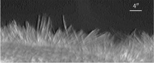
Spicules as seen through the BFI Ca ii H filter on board Hinode/SOT. The image was taken on 2006 November 21 near an active region on the east limb. The image has been rotated, and radial density and emboss filters applied to enhance the visibility of spicules. Only a small region (about 53″ × 22″) from the full SOT FOV is shown.
3.3.2 Evolution and heating of spicules
The life cycle of spicules was the target of numerous studies even before the advent of Hinode (e.g., Rush & Roberts 1954; Lippincott 1957; Nishikawa 1988). One particular focus point has been to find out if spicules are indeed jets and if the spicule plasma is accelerated and/or heated. Such a determination could provide clues about their formation mechanism and how much energy they can carry from the photosphere to higher layers. Most studies reviewed by Beckers (1968) described spicules as apparent mass motions that have a clear ascending phase and a more irregular descending phase (not always observed) with lifetimes of about 5 min and upward (apparent) velocities around 25 km s−1. A “classical” description of spicules was thus established, and even corroborated by later work (e.g., Nishikawa 1988; Christopoulou et al. 2001). Analysis of Hinode data would, however, paint a very different picture.
De Pontieu et al. (2007b) observed spicules with Hinode and found that some behave very differently from the classical description; they are much more violent and shorter lived. Most of these spicules are observed with apparent speeds above 50 km s−1 (some even in excess of 100 km s−1), have lifetimes of 2 min or less, and seemingly fade at the end of their lives, with no downward phase visible in the Ca ii H images. Instead of the classical spicule scenario, De Pontieu et al. (2007b) suggested that spicules are divided into two types, a “type I” that is driven by shock waves and characterized by longer lifetimes and slower apparent speeds, and the more dynamic “type II.” Type-I spicules are believed to be the limb counterparts of active region dynamic fibrils, whose observed properties are well matched by MHD simulations with naturally occurring shocks (Hansteen et al. 2006; Heggland et al. 2007). The origin of type-II spicules is less clear, and De Pontieu et al. (2007b) interpreted their fading from Ca ii H images as a sign of violent heating as they evolve. These findings rekindled the interest in spicules in the context of coronal heating, taking type-II spicules as a promising mechanism to heat the chromosphere and corona.
Not all studies agreed with the existence of two types of spicules. In particular, Zhang et al. (2012b), also using Hinode data, found no clear examples of type-II spicules and claimed that most resembled type-I spicules, questioning any contribution towards coronal heating. However, as part of a statistical study of spicules in different regions, Pereira, De Pontieu, and Carlsson (2012) analyzed the same data sets as Zhang et al. (2012b) and could not reproduce their findings. Analyzing several hundred spicules in quiet Sun, coronal holes, and active regions, Pereira, De Pontieu, and Carlsson (2012) reported that type-II spicules are not only real but they are also the dominant type in most regions of the Sun, except in active regions where type-I spicules dominate. Pereira, De Pontieu, and Carlsson (2012) compared statistics of several properties of spicules in different regions, and found markedly different lifetime and maximum velocity distributions between type-I and type-II spicules, with the latter moving faster and being shorter lived. In figure 11 we show example time sequences of type-I and type-II spicules, together with space–time diagrams built from the intensity at the axis of the spicule. Also shown are distributions (Gaussian kernel density estimates) for the type-I and type-II spicule maximum velocities, lifetimes, and maximum heights calculated from the data of Pereira, De Pontieu, and Carlsson (2012). Type-II spicules were taken from the quiet Sun and coronal hole data sets (N = 344), while type-I spicules were taken from the active region data sets (spicules with observed rise and fall, N = 112); each distribution was normalized.
![Spicules observed with Hinode and their properties. The top two rows show sequences of a type-II spicule in a coronal hole (top) and a type-I spicule near an active region (bottom), each with their space–time diagram on the right [adapted from Pereira, De Pontieu, and Carlsson (2012) by permission of the AAS]. The bottom row shows distributions of type-I and type-II spicule maximum velocities, lifetimes, and maximum heights, calculated from the data of Pereira, De Pontieu, and Carlsson (2012). (Color online)](https://oup.silverchair-cdn.com/oup/backfile/Content_public/Journal/pasj/71/5/10.1093_pasj_psz084/2/m_pasj_71_5_r1_f3.jpeg?Expires=1749038438&Signature=XvffY1KMCjuypZuEByKg~Ovyr-OHqBu5IXyrCkNLQ1LgqrutdiJbfMED94BRbXlTVJSySbMom2fLqUKZkuI6OGKOGxkfcxd1wzJjUADLcPWIf6P0y~MX3WueAcvMCB1sZtsG69c233MUj9fdqqX128GJ~bXIsPxB7E5trLq56YvRYBXe5fYwMCqOYK52QPORCQG5R7ooO~IsO3ge-wy5OKxm4RG4EqIVb0ZImq-NHH3yS13M06Jp27L~a9rTEaONL9FRkkm-rM4iACOQds8hABnA~XmFMuhyd8MXBqRw4Jcj~ef-5X9stow3lYCQwVJWWxrIjozgqYgcU6-ePmIqKA__&Key-Pair-Id=APKAIE5G5CRDK6RD3PGA)
Spicules observed with Hinode and their properties. The top two rows show sequences of a type-II spicule in a coronal hole (top) and a type-I spicule near an active region (bottom), each with their space–time diagram on the right [adapted from Pereira, De Pontieu, and Carlsson (2012) by permission of the AAS]. The bottom row shows distributions of type-I and type-II spicule maximum velocities, lifetimes, and maximum heights, calculated from the data of Pereira, De Pontieu, and Carlsson (2012). (Color online)
Sterling, Moore, and DeForest (2010) studied spicules with Hinode/SOT in a polar coronal hole, and reported fast-moving and short-lived type-II spicules, sometimes accompanied by brightenings in their footpoints just inside the disk. Observing spicules on disk with SOT’s Ca ii H is difficult because of photospheric light contamination, but Anan et al. (2010) were able to follow some bright spicules on the disk close to the limb, and also found that in active region plage, type-I spicules dominate.
Results from Hinode therefore established a new view of the properties of spicules, one that goes against the previously accepted view of classical spicules. If one accepts that most spicules in the Sun are violent type-II spicules, how is that reconciled with previous observations that indicated that spicules have slower rises and longer lifetimes? This question was addressed by Pereira, De Pontieu, and Carlsson (2013), who made use of Hinode data to measure the properties of spicules in original and degraded images (to mimic earlier lower-resolution studies). The authors found that degrading the data significantly influences the measured lifetimes and velocities, because of the lower resolution, the high degree of spicule superposition, and the strong transverse motions of spicules. Their results for the degraded spicule properties agreed very well with the properties of classical spicules. While type-I spicules have properties similar to classical spicules, the two should not be confused. The measured properties of both type-I and type-II spicules converge to those of classical spicules when observed in lower resolution (Pereira et al. 2013).
Tavabi, Koutchmy, and Ajabshirizadeh (2011) studied the diameters of spicules found in Hinode observations and noted the multi-component or multi-threaded nature of several spicules, which was earlier reported by Suematsu et al. (2008a). Tavabi, Koutchmy, and Ajabshirizadeh (2011) claimed to find signatures of type-I and type-II spicules in the diameter distribution, and also argued that the multi-threaded nature of spicules muddles the tracking of an individual spicule with lower-resolution telescopes.
3.3.3 Waves in spicules
Oscillations in spicules have been observed for a long time—see a review by Zaqarashvili and Erdélyi (2009). In addition to the advances in understanding the evolution of spicules, this is a topic where Hinode has also been instrumental, in particular in the discovery of Alfvénic waves in spicules. (We use the term “Alfvénic” to describe waves whose restoring force is mainly magnetic tension.)
Using time series of Ca ii H images, De Pontieu et al. (2007c) reported the discovery of ubiquitous Alfvénic waves that are manifested as transverse motions of spicules. At their typical heights of several thousand kilometers above the limb, spicules are assumed to exist in a low plasma-β environment, and therefore motion in the direction transverse to their axes implies the passage or presence of Alfvénic waves. Given the short lifetimes of spicules, full wave periods were rarely observed. Using a Monte Carlo simulation De Pontieu et al. (2007c) estimated the periods to be between 100 and 500 s. Using typical assumptions for magnetic field strength, spicule density, and their measured transverse velocities of about 20 km s−1, the authors derived an energy flux in the chromosphere of 4–7× 106 cm−2 and about 1.2 × 105 cm−2 in the corona, enough to power the solar wind.
Okamoto and De Pontieu (2011) made use of Hinode observations to study the statistical properties of Alfvénic waves along spicules. They followed 89 spicules and found a mixture of upward-/downward-propagating and standing waves, with the upward-propagating waves more common in the lower part of spicules and standing and downward-propagating waves closer to the tops of spicules. See figure 12 for an example of how Okamoto and De Pontieu (2011) measured the transverse motions and phase speeds of waves along spicules. The authors speculated that upward-propagating waves are produced near the footpoints of spicules, and downward-propagating waves are caused by reflection at the spicule tops in the transition region. Liu, He, and Yan (2014) investigated chromospheric Alfvénic turbulence from these upward- and downward-propagating waves in a few spicules, and supported the findings of Okamoto and De Pontieu (2011), also reporting oscillations with a lower propagation speed, speculating that they could be slow-mode waves.
![Detecting waves in spicules. Left: Example of enhanced Ca ii H filtergram with the detected spicule. Center: Time variation of the horizontal displacements at each height of the spicule. Right: Peak excursions and phase velocities in a space–time diagram. [Reproduced from Okamoto and De Pontieu (2011) by permission of the AAS.] (Color online)](https://oup.silverchair-cdn.com/oup/backfile/Content_public/Journal/pasj/71/5/10.1093_pasj_psz084/2/m_pasj_71_5_r1_f4.jpeg?Expires=1749038438&Signature=bZmKN1oOv6DvqwVJHJkdg-MO1CnMRkTkyXWCW4DJqbRbjwhQQT43vqxygsC6deyN6t53phgM9eChDe4PnY4rak1gdH930U6LH7vy2-PZhvz3SsRn2ngFy5B0okef1InOy985Bt~UCvW4MrsBtKlUhmV0~VbDj0uJMrEkj45slym7SX92vBV5swAKeKX4Y5yM6tQRrl2r9vrXHs~28ZvbGo7EU7Kwg23rFtcjul4h1u5HDBAG3E0xgWR99QhQeUkR~yo2BdK5Q~VnGu309-Gz4NoxJaLPpQxYTUvZpXNuWRJdlqNKMkKBcNQu3rg0JyLSPm1EWQGGrECDPAYoeFRojA__&Key-Pair-Id=APKAIE5G5CRDK6RD3PGA)
Detecting waves in spicules. Left: Example of enhanced Ca ii H filtergram with the detected spicule. Center: Time variation of the horizontal displacements at each height of the spicule. Right: Peak excursions and phase velocities in a space–time diagram. [Reproduced from Okamoto and De Pontieu (2011) by permission of the AAS.] (Color online)
3.3.4 Hinode and IRIS
The disappearance of type-II spicules from Ca ii H filtergrams has been conjectured by De Pontieu et al. (2007b) to be associated with heating, as Ca ii starts to ionize at around 104 K (Carlsson & Leenaarts 2012). While De Pontieu et al. (2011) already linked Ca ii H evolution to later spicule signal in images sampling higher temperatures, it was not until the IRIS mission (De Pontieu et al. 2014b) came online that the matter was settled. Using combined IRIS and Hinode observations, Pereira et al. (2014) studied the evolution of type-II spicules and found that they continue evolving in higher chromospheric and transition region (TR) filtergrams after they disappear from Ca ii H, strongly suggesting that spicules are violently heated to at least TR temperatures. Most spicules will continue evolving in the IRIS filtergrams before eventually falling back down (Pereira et al. 2014; Skogsrud et al. 2015).
Pereira et al. (2014) and Tian et al. (2014b) also reported spicules seen on disk by IRIS, which has been difficult with the SOT Ca ii H filter because of photospheric light contamination. De Pontieu et al. (2014a) used such IRIS disk images of spicules to associate spicular heating with twisting motions.
Combining IRIS with Hinode has been fundamental in piecing together the puzzle of spicule evolution, which neither mission could have achieved on its own. Hinode has provided the high cadence and high spatial resolution necessary to identify the critical early phase of the spicules, while IRIS complemented that information with higher-temperature trajectories of the later phases of spicule evolution and spectral diagnostics.
3.3.5 Summary
Spicules are an enigma whose importance has long been recognized. Observational limitations have for decades dictated limited constraints going into modeling efforts. Identifying their properties and evolution is the first basic step in building a coherent picture of spicules. Hinode afforded a large quantitative step in our knowledge of spicules, arguably the most significant since spicules started to be observed with modern telescopes. Making use of the superior spatial resolution of SOT, its high-cadence observations and the stable seeing-free platform of Hinode, spicules have been observed in unprecedented detail. Spicules were found to be ubiquitous, more dynamic than previously thought, violently heated, and carrying signatures of Alfvénic waves. The heating of spicules can provide clues and input into modeling, whether it is magnetic reconnection, waves, or something else. The Alfvénic wave periods and transverse velocities can be used to estimate energy fluxes at different heights and give insight into how energy is transformed in the solar atmosphere.
Spicules are challenging to observe because they have a very fine spatial structure, evolve in very short time scales, are seen mostly in chromospheric light, and are so abundant at the limb that it is often difficult to discern individual spicules. Ground-based telescopes with higher spatial, temporal, and spectral resolution than Hinode existed even before its launch. The impact of Hinode in spicule studies was made possible because of the nearly continuous, seeing-free nature of the observatory. High-quality time series of spicule observations allowed for a statistical, global view of spicules in different regions and times, and not just limited to a few events.
4 Polar region activities
4.1 Magnetic patches in polar regions
Photospheric magnetic fields of the Sun’s polar region must play an important role in the long-term variation of solar magnetism maintained by a global solar dynamo process and the origin of the fast solar wind that often emanates from a large coronal hole located in the polar region. The average strengths of the Sun’s polar magnetic field inferred from the number of polar faculae (Sheeley 1964) and also measured in ground-based observations of the LOS component of the field (Svalgaard et al. 1978) show a solar cycle variation anti-correlated with that of the sunspot number. Furthermore, their peak strengths at a solar minimum are correlated with the maximum sunspot number of the following cycle (Schatten et al. 1978; Svalgaard et al. 2005). The polar magnetic field strength is therefore considered an important factor in predicting future solar activities. However, the actual evolution process of the Sun’s polar magnetic field was poorly understood because of the following difficulties in conducting polarimetric observations of the polar region. In general (except for sunspots), the amplitude of circular polarization from a magnetized atmosphere is higher than the amplitude of linear polarization. Therefore, the longitudinal (LOS) component of the magnetic field is easier to detect than the transverse component. In a disk center observation and supposing a flux-tube-like structure standing vertically to the surface, the magnetic field is along the LOS. As the FOV moves toward the limb, the magnetic field normal to the surface becomes more and more transversal, and therefore its polarization changes from circular to linear, and the polarization degree decreases. Further, observation from a LOS highly inclined from the local normal suffers from degradation in effective spatial resolution (the foreshortening effect), and the observed region is shifted to a higher altitude (known as the limb darkening effect). In general, the magnetic field is weaker at a greater height, giving weaker polarization. These difficulties combined with variable seeing make ground-based magnetic field observation of polar regions difficult, and hence early observations were only able to measure LOS magnetic fields.
Hinode/SOT-SP has enabled us to conduct high-resolution and high-polarization-sensitivity observation of photospheric magnetic fields, which can mitigate the difficulties of polar region observation. Tsuneta et al. (2008a) derived the vector magnetic field maps of the south polar region in 2007 March using a least-squares fit to the Stokes profiles using the MILOS code (Milne–Eddington Inversion of Polarized Spectra; Orozco Suárez & Del Toro Iniesta 2007) on an SP observation and revealed that the magnetic field landscape in the polar region is filled with a large number of patchy magnetic concentrations (magnetic patches) in which the intrinsic magnetic field strength is higher than 1 kG. The observation showed the coexistence of polar faculae and the large magnetic patches. Although the spatial coincidence of polar faculae and magnetic field concentrations exceeding 1 kG was reported in high-resolution ground-based observations (Okunev & Kneer 2004; Blanco Rodríguez et al. 2007), the Hinode observation revealed the existence of horizontal magnetic-field patches, in addition to the vertical magnetic-field patches similar to those in the quiet Sun (subsection 3.1). This implies that the magnetic field lines of large vertical-field patches expand and fan out with height and produce horizontal fields strong enough to be measured.
Following the first observation of polar regions, the properties of magnetic patches were intensively investigated. Ito et al. (2010) investigated the difference between magnetic fields in the polar region and in an equatorial quiet region near the limb. The field azimuth ambiguity was resolved by assuming that the magnetic field vector is either close to normal or horizontal. They found that the distributions of horizontal magnetic fields in both regions are identical while those of vertical magnetic fields are different. The vertical magnetic field is distributed symmetrically about zero and the flux is balanced in the quiet region. In the polar region the distribution of the vertical component is not symmetrical about zero and one polarity dominates. The unbalanced net flux may lead to field lines connected to some faraway area on the solar surface or to interplanetary space.
Shiota et al. (2012) used a method of automatic detection of magnetic patches and investigated their distributions in terms of magnetic flux, both in the polar and equatorial regions. They found that small vertical magnetic-field patches (magnetic flux <1018 Mx) are balanced in polarity in both kinds of regions. This means that most of the excess magnetic flux of the locally dominant polarity exists in the form of vertical magnetic-field patches whose magnetic flux exceeds 1018 Mx.12 Shiota et al. (2012) also investigated the yearly variation of patch distributions and found that only the distribution of large vertical magnetic-field patches significantly changes with solar cycle activities in the polar regions. These results indicate that solar surface magnetic fields are made of two components: one is patches with horizontal or weak vertical magnetic fields maintained by a continuous and ubiquitous mechanism, such as a convective local dynamo; the other is large vertical magnetic-field patches that comprise the dominant polarity in local as well as polar regions, which may be supplied from flux transport associated with a global solar dynamo mechanism.
As the large magnetic patches of dominant polarity in the polar region can be interpreted as a manifestation of the global magnetic field, Kaithakkal et al. (2013) statistically investigated the relation between large magnetic patches and polar faculae. They showed that polar faculae are embedded in nearly all magnetic patches with flux greater than 1018 Mx, that the faculae are considerably smaller than their parent patches, and single magnetic patches contain single or multiple faculae. They also showed that less than 20% of the total magnetic flux contributed by the large (≥1018 Mx) magnetic patches is accounted for by the associated polar faculae. Hinode observation combined with a deconvolution technique (Quintero Noda et al. 2016) also showed detailed internal plasma and magnetic structures within polar faculae.
These large magnetic patches in polar regions may play an important role in accelerating the fast solar wind. However, the generation and maintenance of the large magnetic patches remain open questions. The vertical kilogauss patches have lifetimes of 5–15 hr (Tsuneta et al. 2008a). The polar faculae are dynamic in nature and the time cadence of SP slit-scan observations of the full FOV is sometimes not sufficient to capture their behavior. Kaithakkal et al. (2015) conducted narrow-FOV, high-cadence SP observations and investigated the association between the formation of vertical magnetic-field patches (lifetime ≤6 hr) and ambient photospheric plasma motions. They found strong converging supergranular flows during the lifetime of vertical magnetic-field patches. They also found that the magnetic patches decay by fragmentation followed by unipolar disappearance (see subsection 3.1), or by unipolar disappearance without fragmentation, in addition to cancelation. Their results suggest that the dominant process in the formation and destruction of large vertical magnetic-field patches is the integration of smaller unipolar fragments and disintegration into smaller unipolar fragments. A similar evolution was seen in detailed studies on SOT-NFI magnetograms of quiet regions near the disk center by Iida, Hagenaar, and Yokoyama (2012, 2015) and Lamb et al. (2013). They investigated the evolution processes of vertical magnetic-field patches in quiet regions by tracking a large number of magnetic patches from their birth to their death. They showed that unipolar appearance and disappearance are considerably more frequent than cancelation and emergence. Considering the connection of magnetic field lines to the upper atmosphere, such evolution of magnetic patches might inject a considerable amount of perturbation along the field lines, which are expected to deposit energy into the upper atmosphere.
As discussed above, the large vertical magnetic-field patches constitute the polar magnetic flux, and must be responsible for driving the solar cycle. The time variations in the distribution of the whole polar regions during the polarity reversal period have been monitored with SP since 2012, which was before the solar maximum of this cycle. Periodic SP observations during a month at the proper timing (March for the south pole and September for the north pole) enabled us to synthesize the magnetic landscape of the whole of both polar regions seen from above the pole, as shown in figure 13 (the details will be reported in D. Shiota & M. Shimojo in preparation). As reported in Shiota et al. (2012), the negative-polarity large patches in the north polar region started to decrease from 2008 at a faster rate than those in the south polar region. In 2012, the negative large magnetic patches in the north polar region almost all disappeared and only medium-scale negative patches remained (figure 13a), while many large positive-polarity patches still existed in the south polar region (figure 13b). As most of the negative magnetic patches in the north polar region had disappeared by 2013, the average magnetic field of the north polar region became almost zero and remained so until 2015. In the map of the north pole in 2016 (figure 13e), we can see a significant increase in the large positive patches at last. On the other hand, the start of the reversal process in the south polar region was delayed until the middle of 2013. However, the process later progressed quickly, and in 2016 (figure 13f) we can see plenty of large negative patches, which indicates that the magnetic distributions have already become similar to the state at the previous solar minimum (Tsuneta et al. 2008a; Shiota et al. 2012). At present, the solar activity is declining and the next polarity reversal is expected to take place earlier in the north polar region because of its low magnetic flux in the present cycle.
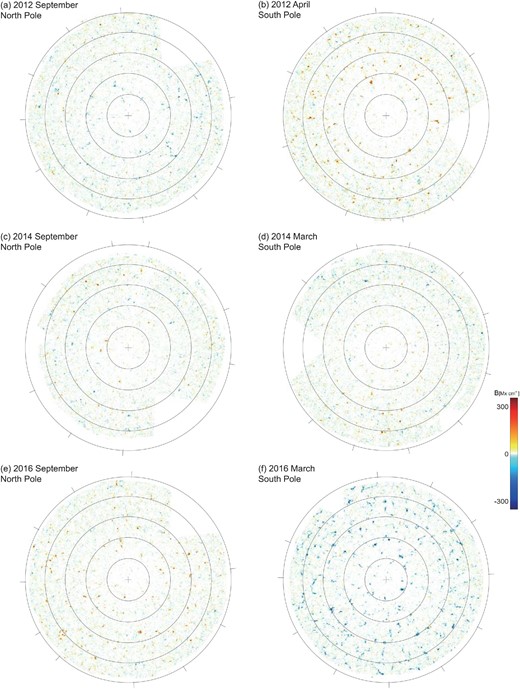
Landscapes of vertical magnetic fields of polar regions from 2012 to 2016 (extracted from D. Shiota & M. Shimojo in preparation). The colors indicate local vertical flux density; the warm colors are positive polarity and the cool colors are negative polarity, as shown in the color bar. The cross symbol is the center of the pole and the circles display co-latitude lines of every 5|$^{\circ}$| in each panel. (Color online)
4.2 Coronal activities in polar regions
While it is well known that coronal activities occur frequently in active regions, we had thought that polar regions are very quiet, based on soft X-ray images obtained with the SXT aboard the Yohkoh satellite (e.g., Shimojo et al. 1996). Our understanding has been revised completely from the polar observations of XRT. The occurrence rate of X-ray jets in a polar coronal hole is estimated to be as high as ∼60 events per day, and the size and lifetime of polar X-ray jets are smaller than those in active regions (Savcheva et al. 2007). The data obtained with XRT also revealed that the average temperature of the X-ray jets in a coronal hole and quiet Sun is around 1 MK (Sako 2014). These observed results indicate that the time cadence and temperature coverage of SXT were not enough to catch polar X-ray jets and might have led to an incomplete view of the coronal activity in polar regions. An example of a polar X-ray jet is shown in figure 14.
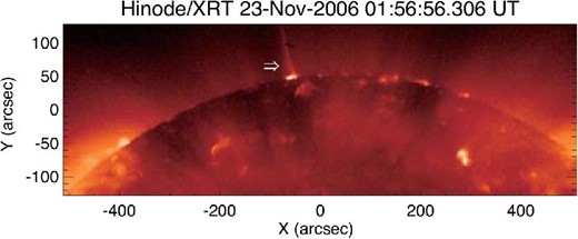
Example (shown by arrow) of a polar X-ray jet observed with Hinode/XRT. (Color online)
Subramanian, Madjarska, and Doyle (2010) investigated equatorial coronal holes and quiet regions, and found that the occurrence rate of brightening at the boundaries of the equatorial coronal holes is higher than in the quiet regions and inside the equatorial coronal holes. Sako et al. (2013) detected 526 X-ray jets and 1256 transient brightenings in the polar regions and in regions around the equatorial limbs. They revealed that the mean occurrence rate of X-ray jets and transient brightenings around the boundaries of coronal holes is higher than in the polar quiet regions, equatorial quiet regions, and polar coronal holes. They also argued that the high occurrence rate cannot be explained from the occurrence rates of emerging and canceling magnetic fields reported in previous studies. Namely, coronal activities in the coronal hole boundary regions might be closely related to the interaction between closed magnetic loops in the quiet regions and the open fields in coronal holes. This is an important issue for understanding the evolution of coronal holes, but our knowledge is still limited.
The high occurrence rate of polar X-ray jets has improved our understanding of the jet phenomena. The X-ray jets occurring in polar coronal holes are also believed to be produced by magnetic reconnection that occurs at a current sheet created between kilogauss patches and emerging flux (Shimojo & Tsuneta 2009). A model of an X-ray jet based on magnetic reconnection predicted the existence of a high-speed flow whose velocity is close to the Alfvén speed (Shibata et al. 1992; Yokoyama & Shibata 1995). Thanks to the high spatial resolution and time cadence of XRT, high-speed flow (∼800 km s−1) was discovered in the slow-speed jet (∼200 km s−1) that might be composed from evaporation flow (Cirtain et al. 2007). Moreover, Sako (2014) suggested a method to identify the force accelerating the X-ray jets (either magnetically driven or evaporation flow) only from the data obtained with XRT. These results revealed that the X-ray jet is a universal phenomenon in the solar corona that is generated by magnetic reconnection. However, we are still puzzled by the motion of the jets. An untwisting motion that might be induced from magnetic reconnection between the twisted and straight magnetic fields is often found in polar coronal jets observed with cooler EUV lines (e.g., He ii) morphologically (Patsourakos et al. 2008; Chen et al. 2009; Nisticò et al. 2009; Moore et al. 2013). On the other hand, one rarely sees a sign of an untwisting motion in the hotter line data obtained with EIS (Kamio et al. 2007; Matsui et al. 2012) and in soft X-ray images.
Raouafi et al. (2008) investigated the relationship between the jets and the plumes (e.g., Saito 1965; Bohlin et al. 1975) using Hinode/XRT and STEREO/EUVI (Wuelser et al. 2004), and found that >90% of the jets were associated with the plume haze and ∼70% of these jets were followed by polar plumes with a time delay ranging from minutes to tens of minutes. From these results, they argued that coronal jets are precursors of plumes. Their interpretation is that the jets result from impulsive magnetic reconnection, while the plumes may be the result of slower magnetic reconnection as implied by the short-lived, small-scale brightenings and jet-like events observed within their footpoints.
In considering the high frequency of coronal activity in polar regions, it seems natural to examine the contribution of X-ray jets to the solar wind. Yu et al. (2014) traced three large polar X-ray jets using the data obtained with Hinode/XRT, SOHO/LASCO-C2, STEREO/COR2 and the Solar Mass Ejection Imager (SMEI; Eyles et al. 2003; Jackson et al. 2004). They found that the high-speed flow of the jets can be traced in the images obtained with the coronagraphs and showed that all three jets have similar mass and energy, ∼1014 g and ∼1029 erg. Based on the diagnostics of physical quantities and the occurrence rate of X-ray jets (Sako et al. 2013), they argued that the jets contribute ∼3.2% of the mass of the solar wind and ∼1.6% of the solar wind energy.
5 Prominences: Structures and flows
Prominences are one of the most striking features of the solar corona. They can be observed clearly in cool spectral lines (e.g., the Hα and Ca ii H lines observed by Hinode/SOT) highlighting their low temperature (∼104 K), which is approximately two orders of magnitude lower than the temperature of the surrounding corona. In tandem with the comparatively low temperature, the density of prominences is two orders of magnitude greater than that of the corona. Prominences, or filaments if they are on the disk, can survive in the corona for weeks, but then they can become destabilized. It is this global stability that is of great importance for space weather forecasting. Even when prominences are globally stable, on small scales they can be incredibly dynamic.
It is fair to say that the study of prominence structure and dynamics with Hinode, especially with SOT, has reinvigorated the field. Just looking at the Astrophysics Data System (ADS) gives 240 papers with the word “prominence” in the title between 1997 and 2006, but 311 between 2007 and 2016. The change becomes even starker if the search is extended to include the word “dynamic” in the abstract: then it goes from 33 to 93 papers over the same periods. One reason for this success is clearly the seeing-free environment that Hinode provides, meaning that we can see the evolution on high spatial and temporal scales over an extended period of time. This has allowed some fantastic data sets to be obtained, including even a prominence eruption observed on 2012 April 16. As a result we have greatly improved our knowledge of prominence dynamics, and it is no surprise that Hinode observations have been challenging our perception of prominences. For in-depth reviews of prominence structure and dynamics, the reader is directed to Labrosse et al. (2010) and Mackay et al. (2010).
5.1 Active region vs. quiescent prominence structuring and dynamics
Prominences can be generally classified into three categories based on the relative proximity to an active region: quiescent, intermediate, and active region. One key aspect for this classification is the strength of the photospheric magnetic field. Active-region prominences are associated with the magnetic neutral lines of the strong magnetic fields that manifest as sunspots and active regions. For regions where the photospheric magnetic field is weak, i.e., far from active regions, the visible characteristics of the prominence change, and as their eruptions are less frequent and less violent, these are quiescent prominences. Figure 15 shows Hinode/SOT observations of an active region prominence (panel a) and an intermediate prominence (panel b). A quiescent prominence is shown in figure 16.
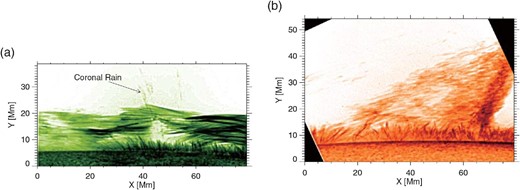
(a) Example of an active region prominence observed on 2007 February 8, 17:24 UT (this also shows coronal rain). (b) Intermediate prominence observed on 2008 January 16, 01:00 UT. (Color online)

Quiescent prominence observed by Hinode/SOT on 2008 September 29 at 10:02 UT. (a) Intensity in the Ca ii H broadband filter; a plume and three downflowing knots are marked on the figure. (b) Doppler velocity in km s−1 as derived from the SOT Hα observations using the method described in Hillier, Matsumoto, and Ichimoto (2017). (Color online)
The dynamics observed in a solar prominence depend heavily on the type of prominence being observed. In general, thread-like structures dominate all types of prominence (Lin et al. 2008; Gunár & Mackay 2015), but there are also many differences. Active-region prominences are dominated by field-aligned flows and MHD waves (Okamoto et al. 2007) of the horizontal threads that make up the prominence, and they also show winding motions (Okamoto et al. 2016). Active-region prominences are more eruptive, and as such have shorter lifetimes than quiescent prominences, which can remain in the corona for weeks. The flow dynamics of quiescent prominences are noticeably different from those of active regions, with a huge range of flows orientated in the vertical direction (Berger et al. 2008). It is also relatively common for quiescent prominences to have vertical structuring. Figure 16 gives an example of a quiescent prominence observed by Hinode/SOT and the many dynamic features they host.
Prominences are known to host a wide variety of oscillatory motions, which are generally interpreted as signatures of MHD waves. Observations of small-amplitude oscillations, interpreted as MHD kink waves, by Hillier, Morton, and Erdélyi (2013) found periods over a wide range from a few minutes to hundreds of minutes with a spectrum that was consistent with the interpretation that these waves were driven by the convection of the photosphere. Schmieder et al. (2013a) found a wave train propagating up through the prominence at a speed of 10 km s−1 with a wavelength of approximately 2000 km. Using magnetic field measurements, which showed the field to be predominantly horizontal, they interpreted the wave train as fast-mode MHD waves. However, Kaneko et al. (2015) presented an alternative explanation for these waves as the result of phase mixing of continuum Alfvén and/or slow waves, which can create the appearance of waves propagating across the magnetic field. For more on prominence wave dynamics in active regions see Antolin et al. (2015a), Okamoto et al. (2015), and subsection 6.1 of this article. For a review of waves in prominences and their use in determining the physical conditions of the prominence see, for example, Arregui, Oliver, and Ballester (2012).
Prominences are full of small-scale flows (Engvold 1981). Chae (2010) presented observations of downflowing knots using Hinode/SOT, finding that they were impulsively accelerated before reaching speeds of ∼10 km s−1 (an example of these flows is shown in figure 16). Using the Multi-channel Subtractive Double-Pass (MSDP) spectrograph combined with Hinode/SOT observations, Schmieder et al. (2010) suggested that due to the similar magnitude to the vertical and line-of-sight flow velocity, some of the observed flows were likely to be material flowing along the magnetic field. In the other direction, prominences also show upward ejection at supersonic speeds of plasma blobs which then follow ballistic motion (Hillier et al. 2011b). These have been interpreted as being driven by magnetic reconnection.
The flow dynamics of intermediate prominences displays some of the characteristics of both types of prominences. Ahn et al. (2010) tracked the flows in an intermediate prominence, finding counterstreaming flows along the prominence spine as well as downflows. The dynamics observed could be characterized by magnetic field lines sagging at an angle of 13° to 39°.
5.2 Prominence thermal and velocity structure as seen with EIS and XRT
Though the rest of this section focuses heavily on the discoveries relating to prominences using Hinode/SOT, it would be unfair not to introduce some of the important results that have been obtained using Hinode EIS and XRT. The first examination of the EUV spectra performed with EIS was presented in Labrosse et al. (2011). The result highlighted the absorption of EUV lines by hydrogen and neutral helium resonance continua and emissivity blocking. By comparison between Hinode EIS spectra of a prominence and 1D non-LTE (local thermodynamic equilibrium) radiative transfer models, they were able to estimate the central temperature (8700 K), central pressure (0.33 dyn cm−2), and column mass (2.5 × 10⁻⁴ g cm−2) for that prominence.
XRT has proved to be a useful tool in understanding the density of a prominence. Using XRT, Schwartz et al. (2015) investigated the prominence emission in soft X-rays, finding that the reduction in the X-ray intensity came from the emissivity blocking as a result of the presence of a large region that was not emitting in X-rays along the line of sight. Heinzel et al. (2008) presented a method to determine the column density of a prominence by comparing soft X-ray and EUV intensities of a prominence, finding column densities of ∼3 × 1019 cm−2. An extension of this method was then applied to multiple prominences, finding mass values in the range 2.9 × 10¹⁴ to 1.7 × 10¹⁵ g.
Coronal cavities, areas of low emission above high-latitude filament channels, have been studied using Hinode. Using the filter ratio method with XRT (Reeves et al. 2012) or using line ratios with EIS (Kucera et al. 2012), the temperatures in cavity regions were found to be ∼1.7 MK.
EIS observations of the Doppler shifts of EUV spectra have also been used to investigate prominence flows. One area this has contributed to is the question of understanding whether the observations that appear to show sections of prominences as rotating columns, known as tornado prominences (Wedemeyer et al. 2013), are really observing a rotating structure. Levens et al. (2015) used EIS to investigate one such prominence and found that at temperatures of log T = 6.0 there was the split Doppler-shift pattern that could be expected for a rotating prominence. However, this possible signature of rotation was not clear in the lower temperatures.
5.3 Prominence plumes and the magnetic Rayleigh–Taylor instability
Prominence plumes are plumes that rise up through the prominence material, and are dark in the cool spectral lines in which prominence material can be observed. These plumes were first observed by Stellmacher and Wiehr (1973) and were simultaneously rediscovered by Berger et al. (2008) and de Toma et al. (2008). These plumes are clearly observed in many quiescent prominences where they rise up at constant velocities, normally between 10 and 30 km s−1, with widths of a few thousand kilometers (Berger et al. 2010). An example of a plume is shown in figure 16.
These plumes often form from bubbles that appear beneath the prominence (Berger et al. 2010). By modeling a prominence as a linear force-free field, that is, by assuming that the prominence is formed of the upward-orientated dips in the magnetic field that has a current but zero Lorentz force and inserting a magnetic bubble underneath it, Dudík et al. (2012) were able to show that the emergence of magnetic flux beneath a prominence qualitatively resembles the observational formation of a bubble beneath a prominence. Berger et al. (2011) used SDO/AIA to analyze two bubbles, finding that they contained a measurable excess of hot plasma but at densities similar to those of the corona. Though some caution needs to be taken, as Gunár et al. (2014) showed that small amounts of cool material in the foreground and background may make the bubble be clear in Hα but not visible in Ca ii H and He ii 304 Å due to their greater optical depth, the resulting prominence-corona transition region emission in 171 Å may result in artificially inflated estimates of temperature if sufficient care is not taken. Due to the large density difference between the prominence and the bubble below, the plumes are hypothesized to be driven by the magnetic Rayleigh–Taylor instability (Ryutova et al. 2010; Hillier 2018).
In trying to understand how this instability develops in prominences, a number of attempts have been made to numerically model these dynamics. Hillier et al. (2011a, 2012a) studied local simulations of the development of the magnetic Rayleigh–Taylor instability in the Kippenhahn–Schlüter prominence model (Kippenhahn & Schlüter 1957). The plumes formed in these simulations were driven by a quasi-interchange mode which allowed magnetic field lines to glide passed each other. The simulated plumes also reached a constant velocity and were quantitatively and qualitatively similar to the observed plumes. A number of authors have now investigated the development of plumes in global prominence models, showing that they can be important for creating vertical structuring (Terradas et al. 2015; Xia & Keppens 2016a, 2016b) and result in convection and turbulence in the prominence (Keppens et al. 2015). Another interesting area of research that has developed from this was demonstrated by Khomenko et al. (2014), who studied the evolution of the magnetic Rayleigh–Taylor instability in a prominence but including the effects of partial ionization, which are important because of the low ionization of the prominence material. These simulations showed that the dynamics driven by the instability could result locally in large velocity drifts between the ionized and neutral species.
A number of attempts have been made to use the linear and non-linear instability conditions to estimate the strength of the magnetic field in prominences. Ryutova et al. (2010) used equation (5) for the linear growth of the instability with measurements of the wavelength and growth rate from the observations and, assuming the angle between the wave vector and magnetic field, were able to infer a magnetic field strength of 6 G. However, as laid out in the discussion of Carlyle et al. (2014) and in Hillier (2016), the growth rate as given in equation (5) is unbounded with wavenumber, so more physics has to be included in the model to give a unique solution for the strength of the magnetic field. Looking at the non-linear stages of the plume development, Hillier, Hillier, and Tripathi (2012b) proposed a model for the compression of prominence material by a plume, and applying this to a prominence plume they were able to determine the plasma β to be ∼0.5.
5.4 MHD turbulence in prominences
The huge range of dynamic flows in prominences take place in a regime with high magnetic Reynolds number and high Reynolds number. These are exactly the conditions that are likely to allow flows to become turbulent, a statement which is somewhat qualitatively verified by the highly complex dynamics of the plumes and flows seen in prominences (Berger et al. 2010). The high spatial and temporal resolution of SOT has provided an opportunity to investigate the role of MHD turbulence in the solar atmosphere.
The simplest concept of turbulence is that of incompressible hydrodynamic turbulence in a homogeneous system, i.e., Kolmogorov turbulence, where dimensional analysis tells us that the velocity power spectra scales as k−5/3 (Kolmogorov 1941). The inclusion of a magnetic field, as with the magnetic Rayleigh–Taylor instability, adds a directionality to the system. In this regime the phenomenological model of MHD turbulence is the non-linear interaction of counter-propagating Alfvén wave packets that resonate with each other, producing new components of the wave packet that are of higher frequency. When the perturbations to the magnetic field are small, weakly non-linear theory holds and results in spectra perpendicular to the magnetic field that scale as |$k_{\perp }^{-2}$|. It is predicted that given a sufficiently large inertial range, the non-linearity of the turbulence would increase until it becomes strongly non-linear. For the fully non-linear case, two competing theories exist: critical balance, which gives spectra of |$k_{\perp }^{-5/3}$| (Goldreich & Sridhar 1995), and increasing dynamic alignment between velocity and magnetic fluctuations with decreasing scale, which gives |$k_{\perp }^{-3/2}$| (Boldyrev 2005).
The first attempt to quantify turbulence in prominences with SOT data was performed by Leonardis, Chapman, and Foullon (2012). Looking at correlations between intensity fluctuations in the prominence, both spatially and temporally, they found power laws. The exponents of these power laws were inconsistent with those predicted by any current MHD turbulence theory, but analysis of the fluctuations revealed intermittency and the multi-fractal nature of the fluctuations, both consistent with the interpretation that quiescent prominences host turbulence. Another interesting feature of the results in this paper was the existence of a break in the spatial power laws at scales of a few thousand kilometers, which is consistent with the scale of many dynamic features of the observed prominence.
Freed et al. (2016) investigated the plane-of-the-sky velocity, obtained through feature tracking, of the same prominence as studied in Leonardis, Chapman, and Foullon (2012). From the measured velocity field they calculated the power spectral density and determined the power spectra, finding exponents of the power-law fit to the power spectra in the range −1 to −1.6. They were also able to place lower limits on the kinetic energy and enstrophy density of the prominence motions as ε ∼ 0.22–7.04 km2 s−2 and ω ∼ 1.43–13.69 × 10⁻¹⁶ s−2.
Complementing these studies, Hillier, Matsumoto, and Ichimoto (2017) investigated the Doppler velocity of a prominence as reconstructed from an SOT Dopplergram (see figure 16b). Using structure functions to analyze the velocity differences, the spectra at larger scales were found to be consistent with strong MHD turbulence (rp/4, where p is the order of the structure function), and consistent with weak MHD turbulence at small scales (rp/2) with the break in the power law at the same scale as that found by Leonardis, Chapman, and Foullon (2012). This transition is the opposite of what is expected from the non-linearity of turbulence increasing as we go to smaller and smaller scales, and as such a different explanation is required. The authors proposed that the break in the power law could be as a result of a transition from the global dynamics of the prominence-corona system to local dynamics in the prominence. Under the assumption that the smaller scales exhibit weakly non-linear MHD turbulence, Hillier, Matsumoto, and Ichimoto (2017) estimated the diffusion across the magnetic field by reconnection diffusion (Lazarian et al. 2012) to be ηrec ∼ 4 × 1010 cm2 s−1, for appropriate parameters for a quiescent prominence, which is of order similar to the estimated ambipolar diffusion, and a few orders of magnitude greater than the Ohmic diffusion. However, when estimating the heating rate as a result of the turbulence this was found to be 10−8 erg s−1 cm−3, which is small and unlikely to be of importance.
5.5 Coronal rain
Coronal rain is a phenomenon strongly related to prominences, and has also become an active field of research in solar physics in the last decade. Since its first description in the 1970s (Kawaguchi 1970; Leroy 1972), this phenomenon was largely thought to be an uncommon, sporadic phenomenon of active regions (Schrijver 2001). This view has dramatically changed thanks to observations that started with Hinode (Antolin et al. 2010), and we now know that it is a very common and recurrent phenomenon.
Coronal rain corresponds to cool and dense flows that appear in a time scale of minutes, mostly in active region coronal loops. The rain can be observed to flow down towards the solar surface in a characteristic rain-like fashion (see figure 15a). The rain, like prominences, is composed of cool and dense cores with temperatures that can reach below 5000 K, with average values of 1–2 × 10⁴ K, and is surrounded by warmer transition-region plasma at 105 K within the hot, coronal environment of a loop. As well as emitting in chromospheric lines, rain has also been observed as EUV absorption features in downflows, sometimes associated with plumes (Levine & Withbroe 1977; Kjeldseth-Moe & Brekke 1998; De Groof et al. 2004; O’Shea et al. 2007), and notably with Hinode/EIS (Tripathi et al. 2009; Kamio et al. 2011; Orange et al. 2013).
The generally accepted origin for coronal rain is that of local cooling within the coronal loop. When radiative losses locally dominate the heating sources, runaway cooling takes place due to the higher radiation efficiency for plasmas the cooler they are. This cooling occurs over a time scale of a few hours under normal coronal loop conditions, and takes the fully ionized hot temperature plasma within a loop to a state of critical equilibrium, warm (1 MK) and over-dense with respect to thermal equilibrium. A local thermal instability is triggered, accelerating the cooling below 1 MK to transition-region and chromospheric values (Van der Linden 1991; Antolin et al. 2015).
Multi-wavelength observations in chromospheric and transition-region lines combining Hinode/SOT, SST, and IRIS suggested that the rain is strongly inhomogeneous at high resolution (Scullion et al. 2014; Antolin et al. 2015). It has a characteristic clumpy morphology along the direction of flow and is multi-stranded in the perpendicular direction, with average sizes of 700 km and 300 km, respectively (although the distribution of the lengths is highly scattered, with values of up to a few tens of Mm). It has been suggested that the multi-stranded morphology is a signature of the thermally unstable modes (van der Linden & Goossens 1991a, 1991b; Antolin et al. 2015).
Coronal rain is observed to accelerate downwards at less than solar gravitational acceleration, to speeds of 100 km s−1 or more (Kleint et al. 2014; Schad 2017). These low acceleration values have been attributed to a redistribution of the gas pressure force downstream of the rain (Oliver et al. 2014, 2016; Kohutova & Verwichte 2017a). While transverse MHD waves are usually observed in rainy coronal loops (Ofman & Wang 2008a), and standing modes can exert an upward ponderomotive force affecting the rain dynamics (Antolin & Verwichte 2011), this force is usually too small to play an important role in the falling speeds (Kohutova & Verwichte 2016; Verwichte et al. 2017b). However, the rain can act as an MHD wave generator if the rain mass is significant compared to that of the loop (Kohutova & Verwichte 2017b; Verwichte & Kohutova 2017; Verwichte et al. 2017b), potentially contributing to the omnipresence of waves in such loops, and hence in prominences as well.
The appearance of coronal rain within a loop depends on the prevalence of cooling over heating within the loop, and therefore is strongly linked to how the loop is heated (Antolin et al. 2010). Numerical simulations have indicated that it is the distribution (Peter et al. 2012) and the steady, high-frequency nature (Müller et al. 2003, 2004) of the heating that leads to such localized cooling events (Hildner 1974; Antiochos & Klimchuk 1991; Antiochos et al. 1999b). The larger the amount of heating at the footpoints, the more it seems to rain. This behavior is especially clear during flares in which strong footpoint heating is observed, and shortly afterwards a massive downpour of rain follows, characterizing the Hα loops associated with flares (Foukal et al. 1974; Foukal 1978; Scullion et al. 2016). When high-frequency heating is maintained for significantly longer than the radiative cooling time, the loop enters a thermal non-equilibrium (TNE) state of repeated heating (evaporation) and cooling (condensation) events (e.g., Kuin & Martens 1982; Karpen et al. 2001), known as TNE cycles or evaporation–condensation cycles. The periods of these cycles depend on parameters such as the loop length, area expansion, the heating scale height, and asymmetries between both footpoints (e.g., Antolin et al. 2010; Mikić et al. 2013; Froment et al. 2018). TNE theory has recently gained increased interest due to the discovery of ubiquitous long-period EUV intensity pulsations in active-region loops (Auchère et al. 2014; Froment et al. 2017) and the accompanying periodic coronal rain (Antolin et al. 2015; Auchère et al. 2018).
5.6 Summarizing prominence dynamics with Hinode
Observations of prominences by Hinode/SOT have revealed that they are an incredibly dynamic environment filled with many complex motions. One key reason for the success of Hinode in observing prominences has been performing observations in optical wavelengths, but in the seeing-free environment of space. This has given us an in-depth view of how flows are created in prominences, and what their existence tells us about the prominence system. These observations show waves, instabilities, non-linear flows, and turbulence, all of which are physical processes that are of interest to researchers in fields outside of prominence study. Therefore, beyond deepening our understanding of prominences, the Hinode observations have also deepened our understanding of the fundamental physical processes of MHD systems.
6 Heating of the upper atmosphere
6.1 Observational signatures of chromospheric and coronal heating by transverse MHD waves
With Hinode playing a central role, a general consensus has been achieved over the last decade regarding the ubiquity of waves throughout the solar atmospheric layers. They are recognized as major players behind the observed chromospheric dynamics, and partly on the heating. However, this consensus is lost in the corona. Here we review the main achievements over the last decade, concentrating on transverse MHD waves (whose main perturbation is transverse to the waveguide), their observational signatures, and dissipation mechanisms in the chromosphere and the corona.
6.1.1 Wave sources, waveguides, and wave modes
Waves emanating from the lower atmospheric layers have global and local sources. Global sources refer to the leakage of internal solar oscillations, and particularly p-modes (Unno et al. 1989). Local sources refer to local excitation processes such as granular convection, convective collapse (Spruit 1979), magnetic buffeting and pumping (Kato et al. 2011, 2016), or magnetic reconnection (Litvinenko 1999). Observations with Hinode and SST give average amplitudes for granular motions on the order of 1 km s−1 (Matsumoto & Kitai 2010; Matsumoto & Shibata 2010; Chitta et al. 2012). Assuming filling factors of 1% and 70%, respectively, for quiet-Sun and active regions, and average inclination angles of 20°–30° for the magnetic field with the granular motion, we obtain upward Poynting fluxes of 3 × 10⁶–1.2 × 10⁹ erg cm−2 s−1 (Fujimura & Tsuneta 2009; Parnell & De Moortel 2012). These values are 1–2 orders of magnitude higher than those required to generate and sustain a corona, 105–107 erg cm−2 s−1 for quiet-Sun and active regions, respectively (Withbroe & Noyes 1977). This fact makes transverse MHD waves good candidates for coronal heating.
The temporal and spatial scales and the nature of the perturbation (whether it is a magnetic or acoustic perturbation initially, and a twist or sideways or longitudinal displacement, and so forth) as well as the local and global structure of the environment (if it is inhomogeneous, stratified, and so forth) will determine the nature and evolution of the generated waves. A perturbation in a given structure on a time scale longer than the information travel time, allowing the structure to accommodate to new equilibria, allows the steady build-up of stress and energy (also known as the “DC mechanism”). A perturbation on a shorter time scale propagates as a wave (also known as the “AC mechanism”). This simple distinction is the basis on which heating mechanisms in the solar atmosphere can, a priori, be separated into two categories: AC or DC heating mechanisms, referring either to waves or to magnetic reconnection as the main heating agent.
In a medium at rest, without gravity and with homogeneous density and magnetic field, local perturbations propagate as MHD slow/fast or Alfvén waves, which are defined by the coupling between different restoring forces: gas/magnetic pressure and magnetic tension. In the lower solar atmosphere the magnetic field concentrates in kilogauss patches (network, see subsection 3.1) or stronger field regions (sunspots) which introduce horizontal magnetic field variations (Raymond et al. 2014). In addition, gravity introduces a vertical density stratification. Such inhomogeneous media define waveguides for MHD waves due to the varying phase speeds. Two main types of waveguides can be found in the solar atmosphere: open and closed magnetic flux tubes, which can themselves be inhomogeneous, and define trapped and leaky (evanescent) waves in an infinite set of different wave modes and complex interactions (Edwin & Roberts 1983).
Why should we care about the nature of a given wave? Because the wave dissipation mechanism depends on the wave mode. For instance, the waves in which gas pressure is a main restoring force will be compressible and therefore can dissipate easily, particularly if they steepen into shocks, while waves for which magnetic tension is the main restoring force (also known as Alfvénic) are mostly incompressible and therefore need an additional mechanism to dissipate their energy, such as MHD turbulence, phase mixing, or mode conversion (see sub-subsection 6.1.6). Furthermore, each wave mode is characterized by unique plasma motions, which leads to a specific set of relations between observables such as intensity, Doppler (LOS) and plane-of-the-sky (POS) velocities, and line width. Studying the characteristics and observational signatures of MHD wave modes is therefore essential for identifying their presence and energetic contribution to the solar atmosphere.
Additionally, the local properties of the environment (the waveguide in this case) introduce specific physical mechanisms that affect wave evolution. Examples of such wave processes are phase mixing, resonant absorption, and mode coupling (see sub-subsection 6.1.2). This implies that to completely characterize an oscillatory signal during observations, not only are spectrometric and imaging information needed, but also the propagation history of a wave (Hansteen et al. 2007). In the solar atmosphere the latter is obtained through co-temporal and co-spatial multi-wavelength observations, tracking the different atmospheric layers in which the wave propagates. Coordinated multi-instrument, multi-wavelength observations are therefore desired. Although such complicated observations are becoming more feasible, lacking the propagation history of a wave makes the interpretation very difficult and often inconclusive. Such an observationally ill-determined problem has often led to debate over the detection and characterization of Alfvénic modes (Van Doorsselaere et al. 2008a; see sub-subsection 6.1.2).
6.1.2 Transverse MHD waves in low-β plasmas and their direct observational signatures
Here we refer to transverse waves as those for which the main perturbation is transverse to the waveguide. These correspond to the Alvénic modes (those for which the magnetic tension is the dominant force, that is, the torsional Alfvén mode and the kink mode) and the fast sausage modes (those for which the magnetic pressure and gas pressure forces dominate over the tension force). Apart from these MHD modes, rotation can also produce torsional oscillations on the condition that it happens on a short time scale relative to the Alfvén travel time. The slow mode is expected to have stronger longitudinal than transverse perturbations, and for these we refer the reader to Wang (2011) and Yuan et al. (2015).
Hinode, in combination with other coronal observations by Coronal Multichannel Polarimeter (CoMP; Tomczyk et al. 2008) and SDO, has clearly shown that transverse MHD waves permeate the corona (Cirtain et al. 2007; Okamoto et al. 2007; Tomczyk et al. 2007; Erdélyi & Taroyan 2008; Van Doorsselaere et al. 2008b; Banerjee et al. 2009; O’Shea & Doyle 2009; Vasheghani Farahani et al. 2009; Kitagawa et al. 2010; McIntosh et al. 2011; Tian et al. 2012; Hahn & Savin 2013). The important role of such waves was first recognized in SOHO/SUMER observations (Carlsson et al. 1997), which showed broad line profiles with strong emission that were not possible to reproduce in a pure hydrodynamic scenario. Observations with Hinode/EIS at higher resolution and sensitivity confirmed this result, and suggested the presence of Alfvén waves (Banerjee et al. 2009) dissipating and driving the fast solar wind (Hahn & Savin 2013). Additionally, with its high resolution and fast cadence, Hinode/SOT confirmed previous results with TRACE (sub-subsection 7.2.1) that high-frequency acoustic waves (5–50 mHz; 20–200 s) could not account for the observed line profiles in the chromosphere, and probably neither for chromospheric heating (Fossum & Carlsson 2005; Carlsson et al. 2007). The latter was, however, refuted by observations at higher resolution with SUNRISE/IMaX (Bello González et al. 2010).
In the following we briefly review the main observational characteristics of transverse MHD waves in low-β plasmas (see figure 17 for a summary).
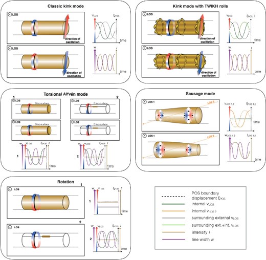
Observational signatures of transverse MHD waves and rotation. Here, we refer to “transverse” waves as those for which the main perturbation is transverse to the waveguide. The “classic” kink mode refers to the kink mode in a loop with a stepwise cross-sectional density. The TWIKH rolls refer to transverse-wave-induced Kelvin–Helmholtz rolls, generated by a kink wave. In the torsional Alfvén wave scenario only the iso-surface of the Alfvén speed within a loop is shown, where the wave is expected to exist. Two scenarios are considered: one in which the iso-surface has constant density throughout, and another in which there is a small density enhancement, whose length scales are much smaller than the wavelength of the wave. Similarly, for the rotation case, the rotation is expected to be uniform over the flux tube with constant density, or over a flux tube with a small density enhancement. For the (fast) sausage mode case, two LOSs are considered: one perpendicular to the loop axis, and one in the loop plane, making an oblique angle with the loop axis. “Internal” and “external” denote motions from plasma internal or external to the flux tube, respectively; vLOS denotes the Doppler velocity along the indicated LOS. (Color online)
Fast sausage waves
These axisymmetric waves, characterized by an m = 0 azimuthal wavenumber, have the gas and magnetic pressure forces in-phase, leading to fast propagation in the corona. Their axisymmetric radial displacement leads to periodic changes in the flux tube cross-section that are for all practical purposes undetectable under normal coronal conditions. However, such area modulation was detected in photospheric and chromospheric flux tubes (Fujimura & Tsuneta 2009; Morton et al. 2011, 2012; Grant et al. 2015; Moreels et al. 2015a; Freij et al. 2016) and was phase-shifted by π with the intensity modulation. Doppler motions were detected when observing at an angle in the loop plane, and were phase-shifted by π/2 with respect to the intensity. Line-width modulation showed double periodicity (Antolin & Van Doorsselaere 2013). Theoretically, sausage waves can only be trapped under normal coronal conditions if they have short wavelengths (1–10 Mm) and periods on the order of seconds to tens of seconds (Nakariakov et al. 2012), which can lead to important non-equilibrium ionization effects drastically reducing the intensity modulation. They are confined to thick coronal flux tubes that are often present in flaring structures and were invoked for explaining oscillatory phenomena such as quasi-periodic pulsations (QPPs; Nakariakov et al. 2003; Tian et al. 2016b; Van Doorsselaere et al. 2016). Long-wavelength sausage waves are therefore expected to be leaky, leading to their fast damping in coronal loops (Williams et al. 2001, 2002; Abramenko & Yurchyshyn 2010), explaining the few reports in EUV lines [e.g., with Hinode/EIS by Kitagawa et al. (2010)].
Kink waves
Characterized by an m = 1 azimuthal wavenumber, these waves produce a transverse displacement of the flux tube (they are the only waves to do so, together with the m > 1 flute modes) and symmetric azimuthal (dipole-like) motion outside the flux tube. Thanks to this property, kink waves are the most easily detected waves among the transverse MHD waves, and are often invoked to explain the dynamics observed in oscillating spicules, prominences, and coronal loops (see sub-subsections 6.1.4 and 6.1.5). Their mixed properties (non-zero magnetic and gas pressure modulation; Goossens et al. 2009) lead to in-phase or anti-phase mild intensity and flux tube area cross-section modulation, depending on the LOS (along the direction of oscillation or perpendicular to it, respectively), with double periodicity (Antolin et al. 2017). In the classical kink mode picture, the case in which no continuous boundary layer transition exists between the interior and exterior of the flux tube, the azimuthal displacement of external plasma is phase-shifted by π/2 with respect to the internal radial displacement of the flux tube (Goossens et al. 2014; Yuan & Van Doorsselaere 2016). In the presence of an inhomogeneous boundary layer (as is expected in the solar atmosphere), these waves become azimuthal Alfvén waves in the flux tube boundary, leading to the process of resonant absorption in the case of standing kink modes (Ionson 1978; Hollweg 1987; Hollweg & Yang 1988; Sakurai et al. 1991). Although the physics is essentially the same, this process is called mode coupling for propagating kink modes (Allan & Wright 2000; Pascoe et al. 2010; Terradas et al. 2010; Verth et al. 2010; De Moortel et al. 2016; Elsden & Wright 2017). The global radial displacement of the flux tube is then converted into local azimuthal displacement in the boundary layer, in which each magnetic surface (defined by the same Alfvén speed) oscillates with the corresponding Alfvén frequency. The process of phase mixing therefore accompanies resonant absorption. Fast damping of the global transverse flux tube displacement is obtained, which is the leading explanation for the observed fast damping following strong external perturbations such as solar flares (Aschwanden et al. 1999; Nakariakov et al. 1999; Goossens et al. 2002; Arregui et al. 2012; De Moortel & Nakariakov 2012), although MHD simulations also show that wave leakage plays a significant role (Miyagoshi et al. 2004; Selwa et al. 2007; Ofman et al. 2015).
The velocity shear produced by the azimuthal flow, particularly in the presence of the resonance, leads to Kelvin–Helmholtz instabilities (KHI; Karpen et al. 1993; Ofman et al. 1994; Poedts et al. 1997; Ziegler & Ulmschneider 1997; Terradas et al. 2008), whose vortices (named TWIKH rolls, for transverse-wave-induced Kelvin–Helmholtz vortices along the loops) produce a strand-like structure in intensity even for low amplitudes (Antolin et al. 2014). TWIKH rolls efficiently mix the external and internal plasma, smoothing out the boundary layer and taking the resonant dynamics to a detectable scale (Antolin et al. 2015a; Magyar & Van Doorsselaere 2016a; Karampelas et al. 2017; Karampelas & Van Doorsselaere 2018). This process is expected to be fueled by resonant absorption, through which a continuous production of vortices and the development of turbulence are obtained (see sub-subsection 6.1.6). In the presence of a radial temperature gradient across the flux tube, emission lines capturing the boundary end up detecting different physical processes, and an apparent decayless oscillation results, contrary to the damping of transverse motions in the core (Antolin et al. 2016). Such dynamics may be able to explain the observed decayless low-amplitude standing kink mode oscillations of coronal loops (Anfinogentov et al. 2013, 2015; Nisticò et al. 2013), although an explanation in terms of continuous footpoint motions as an external driver of loop resonance has also been proposed (Nakariakov et al. 2016). In the TWIKH roll case an out-of-phase (from π/2 to π) relation between the POS motion (radial origin) of the flux tube and the LOS (Doppler) signal (azimuthal origin) is expected (Antolin et al. 2015a), and has been proposed as an explanation for combined Hinode–IRIS prominence observations (Okamoto et al. 2015; see figure 18 and sub-subsection 6.1.5). Various phase relations between observable quantities are expected and are outlined in figure 17 (Antolin et al. 2017).
![Hinode–IRIS observations of a prominence at the limb of the Sun (upper panels) reported by Okamoto et al. (2015) and the suggested physical model (sketch in the middle), based on numerical simulations (lower panels) by Antolin et al. (2015a). The POS motion observed by Hinode/SOT (green curve tracking the prominence thread in the Ca ii H line, in yellow), and LOS velocity observed by IRIS (from the Mg ii k line, in purple) are out of phase (by π) with each other in prominence threads oscillating with a kink wave. A density cross-section of the simulated prominence thread (bottom middle panel) shows the KHI vortices induced by the transverse MHD wave. The vortices’ dynamics are amplified by resonant absorption and show an azimuthal motion due to azimuthal Alfvén waves coupled to the kink wave. Due to the lower density at the boundary, the vortices become increasingly out of phase in time (from π/2 to π) with respect to the center of the flux tube, explaining the observed effect (the simulated time–distance diagram in the bottom right panel matches the phase relation in the top right panel). The KHI develops into turbulence, potentially explaining the observed heating of prominence threads. [Reproduced from Okamoto et al. (2015) and Antolin et al. (2015a) by permission from the AAS.] (Color online)](https://oup.silverchair-cdn.com/oup/backfile/Content_public/Journal/pasj/71/5/10.1093_pasj_psz084/2/m_pasj_71_5_r1_f10.jpeg?Expires=1749038438&Signature=feE0QBt~Hb5O8nmAimws9xuOF9hbDMTjI~Lewe9HG~o9EZYmVkzKCBhVEuFfwsx9e-6o~dYS7cuLA-jhj2g5r0XKbLPAeA9LFrt2bxySIn9v5dAkSiGA~yrLRBwqU3nb-2ZFVfqwnwKCCWpw~H3U~bQAPgGVPCH04Ss06j6EhACDKMtxpPrVo1aAjEsqBceY-33wshmFHmAKhiYv4nhPsUTG261gYVBrhGVXGYloFBNvIoZI9Qz4bMtV6RRfWoVDpyDXK8zZpnUXPjTixjpIHA6vecemjTyJaix1RzlYaJlzufIuCxYhWPEMLYoVq92ON7xyALZ2lfo0-yEInbm9NA__&Key-Pair-Id=APKAIE5G5CRDK6RD3PGA)
Hinode–IRIS observations of a prominence at the limb of the Sun (upper panels) reported by Okamoto et al. (2015) and the suggested physical model (sketch in the middle), based on numerical simulations (lower panels) by Antolin et al. (2015a). The POS motion observed by Hinode/SOT (green curve tracking the prominence thread in the Ca ii H line, in yellow), and LOS velocity observed by IRIS (from the Mg ii k line, in purple) are out of phase (by π) with each other in prominence threads oscillating with a kink wave. A density cross-section of the simulated prominence thread (bottom middle panel) shows the KHI vortices induced by the transverse MHD wave. The vortices’ dynamics are amplified by resonant absorption and show an azimuthal motion due to azimuthal Alfvén waves coupled to the kink wave. Due to the lower density at the boundary, the vortices become increasingly out of phase in time (from π/2 to π) with respect to the center of the flux tube, explaining the observed effect (the simulated time–distance diagram in the bottom right panel matches the phase relation in the top right panel). The KHI develops into turbulence, potentially explaining the observed heating of prominence threads. [Reproduced from Okamoto et al. (2015) and Antolin et al. (2015a) by permission from the AAS.] (Color online)
Torsional Alfvén waves
Contrary to the above two cases, these waves are local in the sense that each iso-surface of Alfvén speed can support a different wave, characterized by the local Alfvén frequency (or speed in the case of open flux tubes). The magnetic tension force is the sole restoring force. They are therefore incompressible, and hence do not lead to intensity modulations in the absence of other physical mechanisms. Their axisymmetric motions (m = 0, as the sausage mode) are purely azimuthal, leading to opposite Doppler signatures from one edge to the radially opposite edge for a given magnetic surface in a flux tube (Goossens et al. 2014). However, if the flux tube is strongly inhomogeneous, contrary to the above cases, the local character of the torsional Alfvén waves would quickly lead to negligible Doppler motions for a given LOS, due to strong LOS integration of different Doppler signals. On the other hand, the same process leads to double periodicity in the line broadening, radially symmetric from one side of the flux tube to the radially opposite side. Furthermore, the local character of these waves makes them unable to transversely displace the entire waveguide. However, if a density enhancement has a spatial scale much smaller than the wavelength of the Alfvén wave, the azimuthal motions of the surface could lead to POS displacements of the small structure. The phase shift between the LOS velocity and the POS motion then depends on the amplitude of the transverse displacement produced by the wave with respect to the loop radius. In general, we would expect this ratio to be small, leading to a π/2 phase shift between the LOS velocity and the POS motion. The localized azimuthal motions of torsional Alfvén waves are again expected to lead to dynamic instabilities such as Kelvin–Helmholtz (Browning & Priest 1984), which would further increase the LOS Doppler superposition and the line width from the KHI turbulence.
The detection of Alfvén waves in the closed configuration of coronal magnetic field lines (torsional or the classical shear Alfvén waves in inhomogeneous and homogeneous media, respectively) has been a constant struggle in the history of solar physics, largely due to their localized nature. The few observational reports of Alfvén waves have based their results on the periodic broadening of spectral lines, and the absence of co-spatial/co-temporal intensity perturbations (Hara & Ichimoto 1999; Jess et al. 2009; McIntosh et al. 2011; Mathioudakis et al. 2013; see sub-subsection 6.1.6). Unfortunately, to date, proper forward modeling of torsional Alfvén waves from 3D MHD simulations is scarce. This would allow a better characterization of their observable features for comparison with observations.
6.1.3 MHD wave mechanisms in the lower solar atmosphere
Waves in photospheric flux tubes are the most straightforward to observe and interpret. Since photons are produced in LTE conditions, intensity is determined by the Planck function, which is completely determined by the local temperature. Based on Hinode/SOT observations, Fujimura and Tsuneta (2009), Moreels and Van Doorsselaere (2013), and Moreels et al. (2015b) have managed to thoroughly characterize the phase relations between observable quantities produced by MHD waves. We refer the reader to these papers and the review by Jess et al. (2015) for details.
Unless being generated in situ through processes such as magnetic reconnection, any wave in the corona initially generated in the photosphere must pass first through the chromosphere, a region that is characterized on one side by the change from gas-pressure-dominated to magnetically dominated dynamics, making this region rich in wave processes, and on the other side by the complicated radiative transfer effects, which complicate the determination of cause and effect from wave dynamics (and therefore also the interpretation of observational signatures).
Density stratification throughout the photosphere and lower chromosphere produces shock steepening in acoustic and slow MHD waves, leading to the conversion of most of their power into heat. The effect of these shocks is seen as one of the primary causes behind the dynamics of type-I spicules (subsection 3.3 and sub-subsection 6.1.4). Parabolic paths and lower-than-gravity deceleration after the shock passage are some of their telltale signatures. The role of the magnetic field in slow-mode waves can be appreciated in inclined waveguides with respect to gravity. The effective gravity reduces the acoustic cut-off frequency, leading to the so-called ramp effect (Michalitsanos 1973; Bel & Leroy 1977; Suematsu 1990; De Pontieu et al. 2004) and the elongation of type-I spicules and other jet-like structure such as fibrils and mottles (De Pontieu et al. 2007a; Heggland et al. 2007, 2009). Density steepening also produces linear mode conversion due to the passage from high-β to low-β plasmas. The increase in phase speeds along flux tubes produces effects such as wave reflection and refraction, which are particularly important for fast modes (Rosenthal et al. 2002; Bogdan et al. 2003). The absence of wave power around magnetic field concentrations such as pores or sunspots observed with Hinode/SOT (Nagashima et al. 2007; Lawrence & Cadavid 2012), the so-called magnetic shadows, finds a partial explanation in these wave processes (Judge et al. 2001; Nutto et al. 2012). The effect is now more generally known as “acoustic power suppression” and involves other mechanisms such as emissivity reduction and local suppression (Chou et al. 2009).
The expected large magnetic field expansion in the lower atmosphere, together with density stratification and the presence of density inhomogeneities along the field, introduces non-linear effects (involving, for example, the ponderomotive force and the deformation of the wave shape) that can produce efficient mode conversion, particularly from Alfvén waves into longitudinal slow- and fast-mode waves. The longitudinal waves can then easily steepen into shocks and drive dense jets of plasma upwards, thereby generating spicules (Hollweg et al. 1982; Kudoh & Shibata 1999; Matsumoto & Shibata 2010; Cranmer & Woolsey 2015; Brady & Arber 2016; Iijima & Yokoyama 2017) and heating both the chromosphere and the corona (Moriyasu et al. 2004; Antolin et al. 2008; Antolin & Shibata 2010). Despite being investigated well theoretically, this process has yet to be directly observed, largely due to the difficulty in detecting Alfvén waves in the lower atmosphere (see sub-subsection 6.1.2). However, many multi-wavelength observational studies exist that strongly suggest this process at work (Fujimura & Tsuneta 2009; Jess et al. 2012; Kanoh et al. 2016), and particularly in the generation of high-frequency transverse oscillations in spicules (He et al. 2009b; Kuridze et al. 2012; Shetye et al. 2016; Shoda & Yokoyama 2018b).
Around the reflection point of the fast modes, a second linear mode conversion is expected to occur due to the strong change of the Alfvén speed with height (Cally & Goossens 2008; Cally & Hansen 2011; Cally 2017). This time, fast modes can mode convert to Alfvénic modes (predominantly torsional Alfvén and kink modes in the presence of density structuring) in a process analogous to the resonant absorption/mode coupling mechanism in dense flux tubes (see sub-subsection 6.1.2). This process can effectively occur throughout the chromosphere and leads to an inherited 5 min period in the Alfvénic waves. This double mode conversion mechanism from p-modes to Alfvénic modes could provide an explanation for recent observations of Alfvénic waves permeating the corona with a 5 min peak in their power spectrum (Morton et al. 2016).
Without the mode conversion mechanisms discussed above, it has been argued that the energy from Alfvén waves generated in the low solar atmosphere is not expected to reach the corona. Particularly for high-frequency waves (with periods of 1–50 s), the Alfvén waves are expected to dissipate most of their energy in the partially ionized chromosphere through ion-neutral collisions (Osterbrock 1961; De Pontieu et al. 2001; Vranjes et al. 2008) and ambipolar diffusion (Arber et al. 2016; Shelyag et al. 2016). The latter seems to be particularly important in the upper chromosphere and in strong field regions (Khomenko & Collados 2012; Martínez-Sykora et al. 2015; Soler et al. 2015) and has recently been proposed as a key ingredient for generating higher-energy spicules (see subsection 3.3 and sub-subsection 6.1.4).
6.1.4 Lessons from spicule observations
Observations primarily with Hinode/SOT and SST have suggested the existence of two types of spicules, a subject which is still under debate (see subsection 3.3). Type-II spicules seem to differ from their type-I counterparts mainly in their higher speeds, heating from chromospheric to at least TR temperatures, their transverse motion (swaying and torsional), and a multi-stranded structure (Suematsu et al. 2008a; Skogsrud et al. 2014, 2015; Pereira et al. 2016). These different characteristics suggest different physical mechanisms at the source and during the evolution of type-II spicules.
The multi-strand structure observed in spicules, both in intensity and Doppler imaging, raises an important question about the real nature of the spicule. Is it the collective group of strands or each separate strand? The collective behavior in the dynamics, in both longitudinal and transverse motions, suggests the former, that is, the spicule as a group of collectively moving strands. This transverse coherence in spicules allows the definition of spicules as “bushes,” the boundaries of which have not, however, been properly defined in observations (Rutten 2012; Antolin et al. 2018b). This transverse coherence suggests waveguides of 103 km or more in width (Skogsrud et al. 2014). Due to the local nature of torsional Alfvén waves, as opposed to collective modes such as the kink mode (or the sausage mode), the observed behavior suggests that the mechanisms responsible for their transverse dynamics are kink modes rather than torsional Alfvén modes. However, for torsional Alfvén modes, as mentioned in sub-subsection 6.1.2, the inhomogeneity introduced by spicules should be much smaller than the wavelength of the torsional Alfvén waves. Observations with Hinode/SOT, however, suggest that this is not likely (Okamoto & De Pontieu 2011; Morton 2014). Nonetheless, the torsional Alfvén wave interpretation was recently supported by Srivastava et al. (2017), albeit a proper forward modeling was lacking, and a clear link between the numerical modeling and the observations was not established.
The combination of the KHI and resonant absorption that accompanies the kink mode (TWIKH rolls) has been shown to produce a strand-like structure, leading to collective behavior whose dynamics and intensity evolution in chromospheric lines seem to match that observed in type-II spicules (Antolin et al. 2018b). However, this mechanism alone seems to fail in reproducing the intensity increase in higher-temperature lines characteristic of these jets. This suggests that other mechanisms, such as magnetic reconnection in the lower atmosphere, probably play a major role in the generation of spicules, and that their morphology may be a by-product of kink modes and dynamic instabilities generated in the process (Kuridze et al. 2016). An example of such a process has been observed with Hinode and reported by He et al. (2009a), in which magnetic reconnection leads to a propagating kink mode along a spicule. Another example is that reported by Jess et al. (2012). A recently proposed and compelling mechanism is ambipolar diffusion, through which the magnetic tension is amplified and generates Alfvénic waves and structures matching type-II spicules (Martínez-Sykora et al. 2017).
The strong transversely oscillating amplitudes, further combined with the high longitudinal speeds found in type-II spicules, suggest an important upward wave energy flux of 4–7× 10⁶ erg cm−2 s−1, sufficient for chromospheric and coronal heating (De Pontieu et al. 2007c, 2011; Srivastava et al. 2017; Martínez-Sykora et al. 2018). Similar amplitudes are also seen in other transversely oscillating structures in the chromosphere, such as fibrils and mottles (Kuridze et al. 2012; Morton et al. 2012), which have been interpreted as kink or fast sausage modes. In the case of sausage modes, a 5% propagation of these compressive waves into the corona would suffice for heating the ambient corona. However, in the case of kink modes, such amplitudes are significantly reduced to 1–7× 10⁵ erg cm−2 s−1 due to the small filling factor of the waves (assuming 5%–15% values; Van Doorsselaere et al. 2014).
6.1.5 Observations of coronal structures: Where does the wave energy go?
The amplitudes of transverse MHD waves in the corona are often reported to be on the order of a few km s−1 under normal non-flaring conditions (De Moortel & Nakariakov 2012; Arregui 2015). Taking usual coronal values for the Alfvén speed and density, the observed energy fluxes are on the order of 1–10 × 104 erg cm−2 s−1. Compared to the chromospheric observations (see sub-subsection 6.1.4), the amplitudes turn out to be at least an order of magnitude smaller. Where does the rest of the energy go? Are we detecting all the wave power? Do transverse MHD waves play any role in the heating of the solar corona?
Several factors have been proposed as possible explanations for the observed energy discrepancy. Besides actual dissipation, the extreme LOS superposition in the corona combined with insufficient instrumental power, and wave processes that concentrate wave power in hard-to-detect spatial scales are all candidates at play that need to be constrained. Among these wave processes, of particular importance is resonant absorption (known as mode coupling in the case of propagating waves), which concentrates wave power in the small inhomogeneous layers of loops in the form of azimuthal Alfvén waves (whose motions are undetectable with imaging instruments). It has been shown that the combination of the LOS superposition and resonant absorption in kink modes leads to an underestimation of the wave energy of 80%–90%, potentially explaining the wave energy gap (De Moortel & Pascoe 2012; Antolin et al. 2017). All these processes readily explain the absence of power in POS transverse displacements, and suggest that the best instruments for detecting the true wave-energy budget in the solar corona are spectrometers.
Observations of wave power in prominences and rainy loops with Hinode/SOT, SST, and IRIS shed light on the role of LOS superposition and insufficient instrumental power. Thanks to their cold and dense chromospheric conditions, prominences allow high-resolution observations into the MHD processes of high- to low-β plasmas. Being high in the corona they also suffer from less LOS superposition (Schad et al. 2016). As such, transverse MHD waves in the corona have been readily detected in these structures by registering the POS motion with high-resolution instruments such as Hinode/SOT and also in Doppler velocities with SST/CRISP (Okamoto et al. 2007, 2015; Berger et al. 2008; Antolin & Verwichte 2011; Lin 2011; Arregui et al. 2012; Kohutova & Verwichte 2016; Verwichte et al. 2017b). In general the waves have lower energy flux, 1–10 × 104 erg cm−2 s−1 (a factor of 10–100), than at chromospheric heights, albeit a large variation with maximum observed values on the order of 1 × 10⁶ erg cm−2 s−1. This suggests that if the waves originate in the lower atmosphere, either an energy cascade to smaller length scales occurs and the waves eventually dissipate and/or a larger role is played in “hiding” the wave energy by wave processes such as mode coupling and resonant absorption. As is seen in coronal-line observations, characteristic signatures include strong damping following external perturbations such as flares (Ofman & Wang 2008b), but also small-amplitude decayless (Ning et al. 2009) and even amplified oscillations (Antolin & Verwichte 2011; Verwichte et al. 2017b). At these higher resolutions the structure appears multi-stranded and, as in spicules, a strong collective transverse motion is also observed. It is also possible that transverse MHD waves are generated in situ through colliding flows, a scenario that has recently been observed by Hinode/SOT and IRIS, supported by numerical simulations (Antolin et al. 2018a).
Coordinated observations with IRIS and Hinode/SOT by Okamoto et al. (2015) have paved the way for how we could actually detect wave heating in action in the corona. In this case the fine dynamics of a prominence was observed in imaging and spectroscopy, allowing the reconstruction of the 3D wave motion and possible dissipation. Strong transverse coherence in transverse MHD oscillations, not only in the POS displacement but also in the LOS velocity (figure 18) were observed, together with prominence threads fading in chromospheric lines and appearing in TR lines, suggestive of wave dissipation and heating. In particular, out-of-phase (from π/2 to π) behavior between the POS motion observed with Hinode/SOT and the LOS velocity detected with IRIS was also reported. All these features were successfully explained with a 3D MHD model of TWIKH rolls, in which the resonant absorption mechanism combines with the KHI and leads to turbulence (Antolin et al. 2015a). It is, however, still unclear how much and on what time scales wave dissipation and heating can be obtained with these mechanisms (see sub-subsection 6.1.6).
While Doppler motions are largely affected by LOS superposition, thereby leading to reduced kinetic energy estimations, line widths are to some extent inversely affected. The increase of non-thermal line widths with height observed by Hinode/EIS in coronal holes is found to be inversely proportional to the quadratic root of the electron density (Banerjee et al. 2009), a fact that has been taken as evidence for propagating Alfvén waves. On the other hand, a decrease of this quantity with height has also been reported, and suggests dissipation of these waves with an energy flux of 6.7 × 10⁵ erg cm−2 s−1, enough to heat the coronal hole and accelerate the solar wind (Hahn et al. 2012; Hahn & Savin 2013). McIntosh and De Pontieu (2012) have shown that the usually observed large non-thermal line widths in the corona tend to increase proportionately with Doppler motions, and suggested a wave origin for this relation in which the spread is produced by the LOS integration effect. On the other hand, torsional Alfvén waves may more readily produce non-thermal line widths proportional to the energy input (Asgari-Targhi et al. 2014). However, the Doppler motions that are expected from them may be even lower and show less coherence than those observed, due to the combination of their local, non-collective nature and the LOS integration effect.
6.1.6 Dissipation of transverse MHD waves in the corona: A cooperation between compressive and incompressible mechanisms
Transverse MHD waves have long been an attractive heating mechanism for both the chromosphere and the corona due to the large generated Poynting flux from convective motions (Uchida & Kaburaki 1974; Wentzel 1974; see sub-subsection 6.1.1). Among these waves, the interest in torsional Alfvén waves has recently been renewed based on the observation of small-scale photospheric vortex motions by Hinode and SST (Bonet et al. 2008; Wedemeyer-Böhm & Rouppe van der Voort 2009; Shelyag & Przybylski 2014; Liu et al. 2019), supported by numerical simulation results (Wedemeyer-Böhm et al. 2012; Kitiashvili et al. 2013; Iijima & Yokoyama 2017; Kato & Wedemeyer 2017). However, dissipation of Alfvén waves in the corona is hard to achieve since the inhomogeneities required for dissipation are expected to be scarce. Also, popular wave dissipation and energy conversion mechanisms such as phase mixing and resonant absorption need the prior existence of a coronal waveguide in order to occur (Cargill et al. 2016), alluding to a chicken and egg problem. Are waves dissipating and maintaining a corona thanks to a more fundamental mechanism generating structure in the corona in the first place? Or can waves self-consistently generate the inhomogeneities they need for dissipation?
In the presence of inhomogeneities that introduce variation of the Alfvén speed at each height, the Alfvén waves readily phase mix (Heyvaerts & Priest 1983; Hood et al. 2002). However, in the linear regime the dissipation rate may be too small in order to sustain radiative and conductive losses (Arregui 2015; Pagano & De Moortel 2017). Numerical models have suggested that small density inhomogeneities along field lines may be created by Alfvén waves themselves (if not already present from longitudinal modes), and that such inhomogeneities are sufficient for wave dissipation via non-linear effects (Hollweg et al. 1982; Kudoh & Shibata 1999). Mechanisms involving the ponderomotive force, wave-to-wave interaction, and parametric decay instability would enhance mode conversion from Alfvén waves to longitudinal modes, leading to shock heating (Sagdeev & Galeev 1969; Goldstein 1978). On the other hand, incompressible effects from MHD turbulence and phase mixing have been suggested to play a dominant role (van Ballegooijen et al. 2011, 2014; Rappazzo 2015; Downs et al. 2016; Matsumoto 2016; Magyar et al. 2017a; Shoda & Yokoyama 2018a; Shoda et al. 2018), a scenario in which, however, dissipation is enhanced by compressive modes. This competition, or rather, cooperation between compressive and incompressible effects is particularly important for the heating and acceleration of the solar wind (Suzuki & Inutsuka 2005; Matsumoto & Suzuki 2014; Laming 2015).
A promising new model that has received increasing attention is that of the TWIKH rolls in the kink wave scenario (see sub-subsection 6.1.2). The KHI induced by Alfvénic waves combines with resonant absorption (in the case of the kink mode) and generates turbulence, thereby distributing the wave energy over a significantly large cross-sectional area of the loop which would otherwise concentrate in the small scales of the loop boundary and other locations of density inhomogeneity (Antolin et al. 2015a, 2016, 2017; Howson et al. 2017; Magyar et al. 2017a) and making it detectable (Okamoto et al. 2015; see sub-subsection 6.1.5). A particularly interesting fact is that the KHI is known to facilitate reconnection and plays a major role in the magnetopause (Nykyri & Otto 2004; Burch & Phan 2016; Moore et al. 2016). It is therefore possible that reconnection occurs in TWIKH rolls, potentially allowing further (impulsive) dissipation of the coronal magnetic field (especially in the presence of twist). In this scenario the waves could act as a stepping stone for other mechanisms (such as reconnection) to take place, through the generation of small scales.
Debate exists on the details of the MHD turbulence in closed and open loop structures (Klimchuk 2015; Velli et al. 2015). Similarly, the turbulence obtained from the recently discovered generalized phase mixing (Magyar et al. 2017a), or from dynamic instabilities such as KHI, both in the kink wave and torsional Alfvén wave cases, is expected to be different (Magyar & Van Doorsselaere 2016b). In all these cases the cascade to smaller dissipative scales may follow specific scaling (different from the Kolmogorov scaling). It is not clear how the intrinsic differences in the turbulent cascades affect the system as a whole. This investigation is challenged by the proper numerical treatment of the turbulent cascade to smaller, dissipative scales (Rappazzo et al. 2008; Howson et al. 2017).
Wave heating is generally thought to be gradual, occurring on time scales set by the wave period, in contrast with the “switch-on” behavior expected from magnetic reconnection (see subsection 6.2), in which large energy release (leading to several MK temperatures) is expected over short temporal and spatial scales. This is certainly the case with the diffusion mechanisms discussed above such as phase mixing, MHD turbulence, and shock heating (from non-linear mode conversion). At small spatial and temporal scales bursty intensity profiles are obtained (that can be interpreted as nanoflares) leading to intensity enhancements on the time scale of a few wave periods (Moriyasu et al. 2004; Antolin et al. 2008; Antolin & Shibata 2010). However, large energy release at small spatial and temporal scales is much harder to achieve, and has therefore been considered as the smoking gun of reconnection-driven models.
6.2 Nanoflare heating: Observations and theory
Understanding how the solar corona is heated to multi-million degree temperatures, three orders of magnitude hotter than the underlying solar surface, remains one of the fundamental problems in space science. Excellent progress has been made in recent years, due in no small part to the outstanding observations from Hinode, but many important questions are still unanswered. The two long-standing categories of heating mechanisms—reconnection of stressed magnetic fields and dissipation of MHD waves—are both still under consideration. There is little doubt that both types of heating occur, and the real issue is their relative importance, which could vary from place to place on the Sun.
It is important to understand that reconnection heating and wave heating are both highly time dependent (Klimchuk 2006; van Ballegooijen et al. 2011; subsection 6.1). The time scale for energy release on a given magnetic field line is likely to be much less than the plasma cooling time, so we can consider the heating to be impulsive. The pertinent question is the frequency with which heating events repeat. If they repeat with a short delay, then the plasma is reheated before it experiences substantial cooling. This is called high-frequency heating, and will produce plasma conditions similar to steady heating if the frequency is sufficiently high. If the delay between successive events is long, the plasma cools fully before being reheated and the heating is considered to be low frequency. The relevant parameter for determining whether the frequency is low, intermediate, or high is the cooling time scale. This varies depending on temperature, density, and field line length, but is typically in the range of several hundred to several thousand seconds.
Impulsive heating events are often called nanoflares. The meaning of the term is not always clear, however. Parker (1988) originally coined the name to describe a burst of magnetic reconnection in tangled magnetic fields. Low repetition frequency was assumed. Subsequently, many studies considered the hydrodynamic consequences of impulsive heating without specifying its cause, and it became convenient to adopt a generic term for any impulsive energy release on a small cross-field spatial scale, without regard to physical mechanism and without regard to frequency. Nanoflare started to be used in this way. That is the definition adopted here.
Another term with various meanings is “coronal loop.” It sometimes refers to an observationally distinct feature in an image, assumed to coincide with a closed magnetic flux tube. A common misconception is that loops are much brighter than the background emission. In fact, they typically represent a small enhancement over the background of order 10% (Del Zanna & Mason 2003; Viall & Klimchuk 2011). Images often give a false impression because the color table assigns black to the minimum intensity, not to zero. Loops are useful to study because they can often be isolated from the background using a subtraction technique. It must be remembered, however, that they represent a small fraction of the coronal plasma and are, by definition, atypical. The diffuse component of the corona is in many ways more important and deserves greater attention than it has received.
The second definition of loop is more theoretical: a curved magnetic flux tube rooted in the photosphere at both ends, with approximately uniform plasma over a cross-section. By this definition, the entire magnetically closed corona is filled with loops. We will use the term “strand” to refer to the theoretical structure, and “loop” to refer to the observational feature. Loops are believed to be comprised of many thinner, unresolved strands.
This short section on observations and theory of nanoflares is nothing like an exhaustive review. Theoretical discussion is restricted to how the plasma evolves in response to a nanoflare. There is no attempt to discuss the theory of heating mechanisms. Citations are representative only and reflect a personal bias. Further information and additional references can be found in Klimchuk (2006, 2015).
6.2.1 Observational discriminators
Some of the earliest evidence for low-frequency nanoflares came from the observation that warm (∼1 MK) loops are over-dense compared to what is expected from steady heating; see the “coronal loops flowchart” (Klimchuk 2009). More recently, coronal researchers have concentrated on four other observational discriminators of low-frequency and high-frequency heating: (1) intensity fluctuations, (2) time lags, (3) emission measure slope, and (4) very hot (>5 MK) plasma.
To understand these discriminators, it is helpful to review the characteristic response of a strand to impulsive heating. The panel at the top left in figure 19 shows the evolution of temperature (solid) and density (dashed) in a strand of 6 × 109 cm total length that is subjected to nanoflares of 100 s duration and 0.15 erg cm−3 s−1 amplitude (triangular heating profile in time). There is also a constant background heating of 10−5 erg cm−3 s−1. Both the impulsive and constant components are uniform in space. The nanoflares repeat every 3000 s, which is much longer than a cooling time, so this is in the low-frequency regime. The simulation was performed with the EBTEL code (Klimchuk et al. 2008; Cargill et al. 2012), and only the last of several cycles is shown, when any influence of the initial conditions is gone. As is well understood, the plasma heats rapidly to high temperature due to the low density at the time of the nanoflare. The subsequent cooling is initially very rapid and dominated by thermal conduction. This then transitions into slower cooling that is dominated by radiation. Density rises during the conduction phase due to chromospheric “evaporation,” and it falls during the radiation phase as plasma drains and “condenses” back onto the chromosphere. The peak in density, and therefore emission measure ( ∝ n2), occurs well after the peak in temperature.
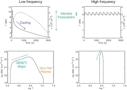
Top panels: Evolution of the strand-averaged coronal temperature (solid) and density (dashed) for low-frequency nanoflares (left) and high-frequency nanoflares (right). Bottom panels: Corresponding time-averaged differential emission measure (DEM) distributions. (Color online)
The panel on the top right shows the same strand that is now heated by a quicker succession of weaker nanoflares. The amplitude is ten times smaller (0.015 erg cm−3 s−1) and the start-to-start delay is ten times shorter (300 s), so the time-averaged heating rate is the same. It corresponds to an energy flux through the footpoints of 7.5 × 10⁶ erg cm−2 s−1, which is appropriate for active regions (Withbroe & Noyes 1977). Despite an equivalent time-averaged heating rate, the behavior is fundamentally different than the first case. Temperature and density now fluctuate about mean values of 3 MK and 3 × 109 cm−3. Because the delay is much less than a cooling time, this is in the high-frequency regime.
6.2.2 Intensity fluctuations
Temporal variations in temperature and density produce temporal variations in emission, which can be used to detect nanoflares and measure their properties. The difficulty is that multiple events are observed together along the optically-thin line of sight. The composite light curve (intensity versus time) from many overlapping strands is nearly steady, even when the individual strands are highly variable. Sizable changes in intensity occur only when an unusually large event occurs or when there is a coherence in events of more typical size. For example, coronal loops are thought to be produced by “storms” of nanoflares, perhaps representing an avalanche process of some kind (e.g., Hood et al. 2016). Attempts have been made to count individual events, but these events are much larger than typical nanoflares, and estimation of their energy is fraught with uncertainty. See Klimchuk (2015) for a discussion of the expected energies of nanoflares (per unit cross-sectional area). Whatever their energy, it is clear that smaller events are much more numerous than larger events and can only be observed in aggregate.
Although individual nanoflares are not generally detectable, their existence can be inferred from the composite emission from many unresolved events. Several approaches have been used. One indication of nanoflares is that the distributions of measured intensities are wider than expected from photon-counting statistics if the plasma were slowly evolving (Katsukawa & Tsuneta 2001; Sakamoto et al. 2008). The distributions also have a skewed shape, as evidenced by small differences between the mean and median intensity (Terzo et al. 2011; López Fuentes & Klimchuk 2016) and by the fact that the intensities are well represented by a log-normal distribution (Pauluhn & Solanki 2007; Bazarghan et al. 2008; see also Cadavid et al. 2016). Skewing of the distributions is expected from the exponential decrease in intensity as strands cool, which can also explain why Fourier power spectra are observed to have a power-law form (Cadavid et al. 2014; Ireland et al. 2015). Finally, the properties of observed light curves are consistent with impulsive heating (Tajfirouze et al. 2016).
6.2.3 Time lags
If a cooling strand is observed with an instrument that can discriminate temperature (narrow-band imager or spectrometer), the emission will peak first in the hottest channel and at progressively later times in cooler channels. Light curves with a clear hot-to-cool progression are typical of many coronal loops. What might seem surprising is that an unmistakable signature of cooling is present even in the nearly steady light curves characteristic of the diffuse corona. Viall and Klimchuk (2012) developed an automated procedure that measures the time lags between observing channels by cross correlating the light curves with varying temporal offset to see which offset maximizes the correlation. Using a combination of SDO/AIA observations and numerical simulations, they concluded that unresolved nanoflares of low to medium frequency are ubiquitous in the corona (Viall & Klimchuk 2012, 2013, 2015, 2016, 2017; Bradshaw & Viall 2016). Note, however, that their results do not preclude the co-existence of high-frequency nanoflares along the same lines of sight.
The longest time delays found by Viall and Klimchuk exceed the predicted cooling times (Lionello et al. 2016; subsection 7.4), though these delays tend to occur in the periphery of active regions, and longer strands are expected to cool more slowly. Also, uncertainties in the optically-thin radiative loss function must be taken into account. The measured delays could indicate a slow change in the envelope of nanoflare energies rather than the cooling of individual strands. Alternatively, they could be due to thermal non-equilibrium (Winebarger et al. 2016). This fascinating phenomenon occurs when steady (or high enough frequency) heating is strongly concentrated in the low corona. No equilibrium exists, and the stand experiences cycles of rising and falling temperature with periods of several hours (Antiochos & Klimchuk 1991). This is usually accompanied by the formation of a cold (∼104 K) condensation, which falls down along one of the strand legs. While this is a likely explanation of coronal rain (Müller et al. 2004; Antolin et al. 2010; see also subsection 5.5) and of prominences (Antiochos et al. 1999b; Karpen et al. 2003), Klimchuk, Karpen, and Antiochos (2010) have argued that it is inconsistent with observations of coronal loops. It has recently been shown, however, that the condensation process can be aborted at modest (∼1 MK) temperatures (Mikić et al. 2013). Such behavior can explain long-period loop pulsations (Froment et al. 2015), which occur in isolated places in some active regions, but might also have more general applicability. Further study is needed.
6.2.4 Emission measure slope
A strand heated by low-frequency nanoflares experiences a wide range of temperatures during its evolution. The emission measure (EM) distribution is therefore very broad. In stark contrast, the EM distribution of a strand heated by high-frequency nanoflares is narrow. The lower panels in figure 19 show the time-averaged differential emission measure distributions of the two examples (corona only; no transition region). The differential and regular emission measures are related according to EM(T) = T × DEM(T). The slope of the distribution coolward of the peak can be approximated by a power law and is a good indicator of nanoflare frequency. Low-frequency nanoflares produce smaller slopes than high-frequency nanoflares (subsection 7.4; Mulu-Moore et al. 2011; Warren et al. 2011a; Bradshaw et al. 2012). A wide range of slopes have been observed in active regions, indicating both low- and high-frequency heating (Tripathi et al. 2011; Winebarger et al. 2011; Schmelz & Pathak 2012; Warren et al. 2012). The uncertainties are substantial, however (Guennou et al. 2013).
It has recently been shown that the range of slopes can be explained if nanoflares occur with a variety of energies and frequencies along the line of sight (Cargill 2014; Cargill et al. 2015; López Fuentes & Klimchuk 2016). The distribution of frequencies must be broad and centered on an intermediate frequency in which the nanoflare delay is comparable to a cooling time (∼1000 s). The EM slope will vary depending on the shift of the distribution toward higher or lower frequencies and possibly also on statistical fluctuations. It is important to note that these same distributions also reproduce the observed range of time lags (Bradshaw & Viall 2016). Figure 20, from a cellular automaton model of López Fuentes and Klimchuk (2016), shows an example of a strand that is heated with a distribution of nanoflare frequencies and energies of the type advocated here.
![Temperature evolution of a strand heated by nanoflares from a cellular automaton model. [Reproduced from López Fuentes and Klimchuk (2016) by permission of the AAS.]](https://oup.silverchair-cdn.com/oup/backfile/Content_public/Journal/pasj/71/5/10.1093_pasj_psz084/2/m_pasj_71_5_r1_f13.jpeg?Expires=1749038438&Signature=Q6X1wB-fAW~Lj07va66zWXOBcYWiMAs94~71xR-sEBnu42iMQBnaZsNZBE5cmKUsPFKzq8Lu~MVlR3dVykVwHNOi2HFgA4~uXnkFihBsh9f~vbp5KTPzMH7UKk9UiUImv9wvfAq5PFa2FfYqf4i0GCJtEvdFY3hl58f-Hkke7p8aFMvL5JgU8rwFJxnoXZMEjp1iJ6rsrmcyef7sjlWkewh42K0E3jjI6HTCMn0EU0MDPGp4PfUigP6CnWnKWPs2n9TKRB-agZP~K7Tf3oOMLymm5xIeF30wbABiqYtTtyxFUmqJ44~QoJWtz8rmD74s73gCgGXFsurxybldCvfvbQ__&Key-Pair-Id=APKAIE5G5CRDK6RD3PGA)
Temperature evolution of a strand heated by nanoflares from a cellular automaton model. [Reproduced from López Fuentes and Klimchuk (2016) by permission of the AAS.]
6.2.5 Very hot (>5 MK) plasma
The presence of very hot plasma in the corona is a strong indication of low-frequency nanoflares, since the heating rate needed to maintain steady plasma at such temperatures is extreme. For example, a strand of total length L = 1010 cm requires an energy flux through the footpoints of 4 × 10⁸ erg cm−2 s−1 to produce a steady apex temperature of 10 MK. If this energy were supplied by stressing of the field by footpoint motions, as envisioned by Parker (1988), it would require continuous horizontal velocities in the photosphere of more than 10 km s−1 (assuming an active region coronal field strength B = 100 G). This is more than an order of magnitude faster than observed. Higher temperatures and weaker fields would require even faster flows, since v ∝ T7/2/(B2L).
We refer to very hot plasma as the “smoking gun” of low-frequency nanoflares. Such plasma is difficult to observe, however, because it is expected to be very faint. As figure 19 shows, the plasma cools rapidly and persists for only a short time. Its density is low because evaporation has not had time to fill the strand. Both factors contribute to a time-averaged emission measure that is very small. There have been multiple investigations to detect very hot plasma, most of them successful (Ko et al. 2009; McTiernan 2009; Patsourakos & Klimchuk 2009; Reale et al. 2009a, 2009b; Schmelz et al. 2009a, 2009b; Sylwester et al. 2010; O’Dwyer et al. 2011; Testa et al. 2011; Warren et al. 2011a, 2012; Teriaca et al. 2012a; Testa & Reale 2012; Del Zanna & Mason 2014; Ugarte-Urra & Warren 2014; Caspi et al. 2015; Parenti et al. 2017; Viall & Klimchuk 2017). Of particular note are the results from the EUNIS rocket spectrometer, which observed pervasive Fe xix emission (∼9 MK) in an active region (Brosius et al. 2014). Non-equilibrium ionization can further diminish the intensity of very hot spectral lines (Golub et al. 1989; Reale & Orlando 2008; Bradshaw & Klimchuk 2011), but such effects do not impact thermal bremsstrahlung emission observed in hard X-rays (Ishikawa et al. 2014; Hannah et al. 2016). Marsh et al. (2018) found that hard X-ray continuum spectra from the FOXSI sounding rocket and NuSTAR mission are consistent with low-frequency nanoflares.
6.2.6 Conclusions
In summary, the variety of different techniques for diagnosing coronal heating support the view that nanoflares occur with a wide range of energies and frequencies. Such a picture can reconcile observations that would otherwise seem to be contradictory. For example, Warren, Winebarger, and Brooks (2012) measured the EM slopes in small sub-fields within 15 active regions and found a range of values indicating high-frequency heating in some cases and low-frequency heating in others. Viall and Klimchuk (2017) studied these same sub-fields using their time lag technique and found clear evidence of low- and intermediate-frequency heating in every case, including those with steep slopes. All of the sub-fields also show evidence of very hot plasma, which can only come from low-frequency nanoflares. It seems that nanoflares of all frequencies are present, and that different techniques are sensitive to different parts of the frequency distribution.
Much more work needs to be done to determine how nanoflares are distributed in frequency and energy, and how these distributions vary in space and evolve with time. Among the important questions are the following: What causes the collective behavior responsible for loops? When does high-frequency heating persist for long enough to produce thermal non-equilibrium, with full or aborted condensations? What is the physical mechanism responsible for the heating?
We close by stressing the importance of studying emissions of very high temperature (>5 MK). Such emission gives direct information on the energy-release process during low-frequency heating, when there is the least observational ambiguity. Much of the plasma at traditional coronal temperatures (∼2 MK) has either cooled dramatically, in which case valuable information about the heating mechanism has been lost, or else has been evaporated from the chromosphere and is only an indirect by-product of the heating. Emission line spectroscopy of very high temperature plasma is especially desirable. As already stressed, nanoflares are observed in aggregate due to line-of-sight overlap and finite spatial resolution. Only spectroscopy can sort out the properties (temperature, velocity, etc.) of non-uniform plasmas.
7 Active regions
7.1 Sunspot structure
Sunspots, the dark features on the surface of the Sun due to the suppressed convection owing to the presence of a strong magnetic field in them, contain multiple small-scale structures in the central darkest part, the umbra, and in the less-dark region surrounding the umbra, the penumbra (figure 21). The magnetic, thermal, and flow structures of sunspots were extensively studied in the pre-Hinode era, but multiple questions pertaining to sunspot fine structure, their formation, evolution, and decay, remained open, requiring a closer look. Some of these questions were proposed to be pursued by Hinode/SOT. For example, what are the internal structures of basic umbral and penumbral features (i.e., umbral dots, umbral dark area, light bridges, penumbral filaments, spines, penumbral bright grains) of sunspots and how are these basic umbral and penumbral structures formed and maintained? What drives the Evershed flow in sunspot penumbra in the photosphere and the inverse Evershed flow in sunspot penumbra in the chromosphere? How do the basic sunspot structures disintegrate in magnetic fragments and diffuse to the quiet Sun? How do moving magnetic features form and what is their role in sunspot decay? Are umbral dots, light bridges, and penumbral filaments (magneto)convection cells, as suggested by recent numerical modelings?
![Continuum intensity image of a sunspot observed by Hinode/SOT-SP [reproduced from Tiwari et al. (2015) by permission of ESO]. Locations of a couple of umbral dots (UDs), penumbral filaments (PFs), spines, penumbral grains (which are actually heads of filaments), and a light bridge (LB) are pointed to by arrows. A larger arrow in the center of the sunspot umbra points to the direction of the solar disk center. The scale of the picture is 64″ × 64″. To clearly visualize the penumbral features (including dark lanes on penumbral filaments), a zoomed-in view of a small FOV of the sunspot penumbra, outlined by the dash-dotted box, is displayed on the right. (Color online)](https://oup.silverchair-cdn.com/oup/backfile/Content_public/Journal/pasj/71/5/10.1093_pasj_psz084/2/m_pasj_71_5_r1_f14.jpeg?Expires=1749038438&Signature=FYWBiMM8cWq2-r4MoCrtrb~RwLZx90WRyJ4F~zBoweI1b3Ier3xXra1W~4N74VCbpqhoXFGcBAo3UYXgAcHRNpxOQMBHhlDB656Tao7oWHxdHUnkNPmF9ai9ycunWEQljd9dhxtFv6azYcwo0U0wGgs3e9X7SPQxO3WoSMdwObftU9jzsEwgz-xl4xGAm-MnjryihCHXA0XYZ2EYZ~Y6hHudyJ07zEqeagQWcxRbe4s2rC44SNa-myqUb~x2rGkw7U-W7Q83IYpHtP5bHKsufyQQgAgaANZ93s5LBxhKcl0AiOXfs12LkmVjA9mjo6sZB9K3Q1fyD5uDBC8Q1rtk8g__&Key-Pair-Id=APKAIE5G5CRDK6RD3PGA)
Continuum intensity image of a sunspot observed by Hinode/SOT-SP [reproduced from Tiwari et al. (2015) by permission of ESO]. Locations of a couple of umbral dots (UDs), penumbral filaments (PFs), spines, penumbral grains (which are actually heads of filaments), and a light bridge (LB) are pointed to by arrows. A larger arrow in the center of the sunspot umbra points to the direction of the solar disk center. The scale of the picture is 64″ × 64″. To clearly visualize the penumbral features (including dark lanes on penumbral filaments), a zoomed-in view of a small FOV of the sunspot penumbra, outlined by the dash-dotted box, is displayed on the right. (Color online)
High spatial resolution, precise, and high signal-to-noise observations by Hinode/SOT have contributed extraordinarily to understanding of sunspot structure and dynamics in the first eleven years by providing new information about many sunspot features, including umbral dots, light bridges, penumbral filaments, and moat regions, and have disclosed their internal structures. Hinode has helped to address several of the abovementioned questions, and opened new directions. See Solanki (2003) for a detailed review of sunspot structure and for open questions thereon before the Hinode era.
In this subsection we review some of the latest developments, achieved from data of unprecedentedly high quality obtained by Hinode, in establishing (mostly photospheric) thermal, flow, and magnetic properties of sunspot structures at both small and global scales. Note that although works on umbral dots, light bridges, moving magnetic features, umbral/penumbral jets, and formation/decay of sunspots are reviewed, more extensive detail is given on the fine structure of the sunspot penumbra, the most complicated magnetic structure on the surface of the Sun, the understanding of which Hinode has contributed to most significantly. We also discuss some questions that have emerged as a result of these new observations, i.e., about sunspot structure, dynamics, and their connection with the upper atmosphere, and point out the need for multi-height/multi-temperature observations at a higher spatial resolution and cadence that are needed to answer them and that are anticipated from future-generation solar telescopes, e.g., DKIST and the next Japan-led solar space mission (SOLAR-C_EUVST).
For past reviews on the structure of sunspots, please see Moore (1981), Spruit (1981), Moore and Rabin (1985), Schmidt (1991), Sobotka (1997), Solanki (2003), Thomas and Weiss (2004, 2008), Scharmer (2009), Tritschler (2009), Borrero and Ichimoto (2011), and Rempel and Schlichenmaier (2011). In recent years MHD simulations have made significant progress in reproducing many aspects of the small-scale structures of sunspots (Hurlburt et al. 1996; Hurlburt & Rucklidge 2000; Schüssler & Vögler 2006; Heinemann et al. 2007; Scharmer et al. 2008; Rempel et al. 2009; Rempel & Schlichenmaier 2011; Rempel 2012). In this review we mainly focus on the observational results and, when suitable, mention relevant simulations.
7.1.1 Umbral dots and light bridges
Sunspot umbrae often contain light bridges (LBs) and umbral dots (UDs); both are enhanced bright structures inside dark umbrae, magnetoconvection being a proposed mechanism of heat transport in them (Weiss 2002; Schüssler & Vögler 2006; Kitai et al. 2007; Watanabe et al. 2009; Watanabe 2014). Using Hinode/SOT-SP data, Riethmüller, Solanki, and Lagg (2008) detected upflows of 800 m s−1 and a field weakening of some 500 G in UDs; see also Sobotka and Jurčák (2009) and Feng et al. (2015) for a comparison of central and peripheral UDs. Riethmüller et al. (2013) further analyzed the same sunspot data using a more sophisticated inversion technique and detected systematic diffuse downflows surrounding UDs, consistent with the downflows seen by Ortiz, Bellot Rubio, and Rouppe van der Voort (2010) in a few UDs of a pore. Riethmüller et al. (2013) further found that upflowing mass flux in the central part of UDs balances well with the downflowing mass flux in their surroundings. Evidence of dark lanes in UDs, as predicted by MHD simulations of Schüssler and Vögler (2006), was reported by Bharti, Joshi, and Jaaffrey (2007) and Rimmele (2008). On the other hand, Louis et al. (2012) and Riethmüller et al. (2013) could not detect it, thus questioning the magnetoconvective nature of UDs. Furthermore, MHD simulations suggest concentrated downflows at the UD boundary, not found in observations so far.
Light bridges, often apparent as a lane of UDs, separate sunspot umbrae into two or more parts of the same-polarity magnetic field. They can be divided into “granular” photospheric substructures (e.g., Lites et al. 1991; Rouppe van der Voort et al. 2010; Lagg et al. 2014), “faint” LBs (Lites et al. 1991; Sobotka & Puschmann 2009), or “strong” LBs (Rimmele 2008; Rezaei et al. 2012). Similar to UDs, the magnetic fields in all types of LBs are more inclined from vertical as compared to their surroundings (Jurčák et al. 2006; Katsukawa et al. 2007a; Lagg et al. 2014; Felipe et al. 2016); similar to the convergence of the spine field over penumbral filaments (described later), the umbral field converges above LBs. Supporting their convective nature, upflows in the central parts of LBs and surrounding strong downflows have been observed (Rimmele 1997; Hirzberger et al. 2002; Louis et al. 2009; Rouppe van der Voort et al. 2010; Lagg et al. 2014). Dark lanes have been detected in LBs using Hinode data by, e.g., Bharti, Joshi, and Jaaffrey (2007) and Lagg et al. (2014), thus supporting the magnetoconvective nature of LBs. Lagg et al. (2014) found field-free regions in granular LBs with similarities to “normal” quiet-Sun granules, thus suggesting that, unlike other umbral features (i.e., UDs and other types of LBs), granular LBs could be made by convection from deeper layers. In recent work using Hinode/SOT-SP time series of a sunspot, Okamoto and Sakurai (2018) found an LB to have the strongest magnetic field over the sunspot.
Several small-scale jet-like events in connection with UDs and LBs have also been reported using Hinode data (e.g., Shimizu et al. 2009; Shimizu 2011; Louis et al. 2014; Bharti 2015; Toriumi et al. 2015b; Yuan & Walsh 2016).
7.1.2 Structure of sunspot penumbral filaments
With the presence of rapidly varying field, flow, and thermal properties, in both radial and azimuthal directions, sunspot penumbrae undoubtedly represent the most complicated and challenging structures on the solar surface. Penumbrae are made of copious thin bright filaments (Title et al. 1993; Rimmele 1995; Langhans et al. 2005; Ichimoto et al. 2007b; Borrero & Ichimoto 2011) and a dark spine field (Lites et al. 1993). See also Su et al. (2009a) and Tiwari, Venkatakrishnan, and Sankarasubramanian (2009b) for the fine-scale distribution of local twists and current densities in sunspot penumbrae, and Tiwari et al. (2009a) and Gosain, Tiwari, and Venkatakrishnan (2010) for the effect of polarimetric noise in estimating these parameters using Hinode data.
According to theoretical expectations (Cowling 1953; Spruit 1977; Jahn & Schmidt 1994), the presence of a strong magnetic field of 1–2 kG should prohibit convection in sunspot penumbrae, thus keeping them dark, similar to umbrae. As penumbrae have a brightness of some 75% of the quiet-Sun intensity, some form of convection takes place therein. It may be radial, i.e., upflows take place in the inner penumbrae and downflows in the outer penumbrae. Or there could be azimuthal/lateral convection, in that upflows take place all along the filament’s central axis and downflows along the sides of the filament. Or the convection in penumbrae may be a combination of the above two (Borrero & Ichimoto 2011). The presence of radial convection was evidenced by, e.g., Rimmele and Marino (2006), Ichimoto et al. (2007b), and Franz and Schlichenmaier (2009, 2013). Support for azimuthal convection was found by Ichimoto et al. (2007b), Zakharov et al. (2008), Bharti, Solanki, and Hirzberger (2010), Joshi et al. (2011), Scharmer et al. (2011), Scharmer and Henriques (2012), Tiwari et al. (2013), and Esteban Pozuelo, Bellot Rubio, and de la Cruz Rodríguez (2015), while other researchers could not detect such downflows (Franz & Schlichenmaier 2009; Bellot Rubio et al. 2010; Puschmann et al. 2010). Furthermore, convection in the penumbra can take place in the presence of a strong magnetic field (Rempel et al. 2009; Rempel & Schlichenmaier 2011; Rempel 2012), or in a very weak field, or in the absence of it (field-free gaps; Scharmer & Spruit 2006; Spruit & Scharmer 2006).
By using Hinode/SOT-SP data of a sunspot (leading-polarity sunspot of NOAA AR 10933) observed almost on the solar disk center (μ = 0.99) on 2007 January 5 (during 12:36–13:10 UT), Tiwari et al. (2013) explored the fine structure of penumbral filaments. Tiwari et al. (2015) then studied global properties of the same sunspot in light of the fine structure of filaments and spines, and sorted out the thermal, velocity, and magnetic structures of the whole sunspot. In the following we summarize some of the main results found in these papers, with appropriate discussion and additional topics included. Interestingly, different aspects of the Hinode data for this particular sunspot have been studied by several researchers, which has resulted in many other publications (e.g., Kubo et al. 2008b; Franz & Schlichenmaier 2009; Tiwari 2009, 2012; Tiwari et al. 2009b; Venkatakrishnan & Tiwari 2009, 2010; Katsukawa & Jurčák 2010; Borrero & Ichimoto 2011; Franz 2011; Riethmüller et al. 2013; van Noort et al. 2013; Joshi et al. 2017).
For exploring the internal structure of sunspot penumbra, Tiwari et al. (2013, 2015) used the spatially-coupled inversion code (see sub-subsection 3.1.1) implemented in the SPINOR code (Frutiger et al. 2000), which returns depth-dependent physical parameters, based on their response functions to the used spectral lines. Tiwari et al. (2013, 2015) used a pixel size of 0|${^{\prime\prime}_{.}}$|08 and the structures down to the diffraction limit of the telescope were resolved. The physical parameters returned from the inversion are temperature T, magnetic field strength B, field inclination γ, field azimuth φ, line-of-sight velocity vLOS, and a micro-turbulent velocity vmic. Before the velocities were inferred, a velocity calibration was done by assuming that the umbra, excluding UDs, was at rest. Maps of the sunspot in a few selected physical parameters from the inversion are shown in figure 22.
![Four selected maps of physical parameters of the leading positive magnetic polarity sunspot from AR 10933, observed by Hinode/SOT-SP and inverted using spatially coupled inversions. (a) T map; a black arrow points to the solar disk center. (b) B map. (c) γ map. (d) vLOS map. Color bars for the parameters are attached to the right of each panel, and are scaled to enhance the visibility of spatial variations in the parameters. [Reproduced from Tiwari et al. (2015) by permission of ESO.] (Color online)](https://oup.silverchair-cdn.com/oup/backfile/Content_public/Journal/pasj/71/5/10.1093_pasj_psz084/2/m_pasj_71_5_r1_f15.jpeg?Expires=1749038438&Signature=L8718myIIkmzLYT9ky2TzNh1VeGXYWvFzdArRbiKDmphS9P8Gwkgc1xjt6BNED100IKopNYuKSkDH18H3ixugCSzAI3T5bSclz7-JUgWmY1ExLIT2sKnknmE4JGEE9a-iE6SlDxndKX7CGsqqc73itMixecgXjxFcgONwgNXqYkEAWRhwb-NSPSM3e7CdxKfNH2qw-HzwJIBkk8C6nwyIGLRsSTVdg7y~2FTYC-CHO0KYlZhcU4uYU7wbIV3fPq-pi7z2A3q9nMdd4ODxkV12ktB6SB-PNh--VByoAl-39ZsKOfKtGsbmdIuD9Erl1bUPdHW~J09nFVg9rTGS55i-Q__&Key-Pair-Id=APKAIE5G5CRDK6RD3PGA)
Four selected maps of physical parameters of the leading positive magnetic polarity sunspot from AR 10933, observed by Hinode/SOT-SP and inverted using spatially coupled inversions. (a) T map; a black arrow points to the solar disk center. (b) B map. (c) γ map. (d) vLOS map. Color bars for the parameters are attached to the right of each panel, and are scaled to enhance the visibility of spatial variations in the parameters. [Reproduced from Tiwari et al. (2015) by permission of ESO.] (Color online)
Selecting penumbral filaments
From the maps of the physical quantities returned from the inversions of the Hinode/SOT-SP data of a sunspot, Tiwari et al. (2013) were able to isolate penumbral filaments. However, because a single-parameter map was not sufficient to track full filaments, e.g., filament heads (the “head” of a filament is the part of the filament nearest to the sunspot umbra) were clearly visible in T and vLOS maps but could not be detected in γ maps, and the tails (the “tail” of a penumbral filament is the part of the filament farthest from the sunspot umbra) of filaments could not be detected in T maps, Tiwari et al. (2013) combined T, vLOS, and γ maps for selecting filaments. The selected penumbral filaments were destretched and straightened using bicubic spline interpolation and normalized to a certain length. To reduce fluctuations and to extract common properties for all filaments, they averaged filaments after sorting them into inner, middle, and outer filaments. Before the work of Tiwari et al. (2013), the full picture of a penumbral filament was not known (see, e.g., Borrero & Ichimoto 2011).
Uniformity of properties in all penumbral filaments and the “standard filament”
The selected filaments showed similar spatial properties everywhere, in the inner, middle, and outer parts of the sunspot penumbra. Therefore, Tiwari et al. (2013) averaged all selected penumbral filaments to create a “standard penumbral filament.” In figure 23 we display a few physical parameters of the standard filament at the optical depth unity. Please see Tiwari et al. (2013) for plots of their depth dependence and quantitative properties.
![Maps of five physical parameters of the standard penumbral filament, all at the surface of unit optical depth. Quantitative values along the longitudinal dashed line at the central axis of filaments and at three transverse cuts can be found in Tiwari et al. (2013). The total width including the surrounding mostly spine field is 1${^{\prime\prime}_{.}}$6; the width of the filament itself, outlined for reference in the vLOS map by two longitudinal dotted lines, is 0${^{\prime\prime}_{.}}$8. [Reproduced from Tiwari et al. (2013) by permission of ESO.] (Color online)](https://oup.silverchair-cdn.com/oup/backfile/Content_public/Journal/pasj/71/5/10.1093_pasj_psz084/2/m_pasj_71_5_r1_f16.jpeg?Expires=1749038438&Signature=yrnf9Izdx9arL6MU4WAt7sUXBcKj-nCktsL3Nxbd8StdFVZRPRp~aAT83zcks~XFanYOCfKvgG2AIQXGM9alpZAqxhs2fbN-C2VkUvZ~Q71IklTTFTLtyS~LQmcJGSgfv9dWw~H796mXKvb82HQqUG8bvVqW8cq6v9Pu1GZBG7MU8~sBz~2x2PFfUw~zAXA5HzU0vFTDj9E4cPYo7ZeydLRw8sectk~b2zmrBUBSGcuiIyiXpEYSZYnOyztNKbhhAUEOpmtlEl8-1TRSAo1EstIMlXQVQeTJ1Ucmf5TdWiY4SrJhnXJbstanHXMEAAZvI~jiGBIACl77EBAYaMrJvA__&Key-Pair-Id=APKAIE5G5CRDK6RD3PGA)
Maps of five physical parameters of the standard penumbral filament, all at the surface of unit optical depth. Quantitative values along the longitudinal dashed line at the central axis of filaments and at three transverse cuts can be found in Tiwari et al. (2013). The total width including the surrounding mostly spine field is 1|${^{\prime\prime}_{.}}$|6; the width of the filament itself, outlined for reference in the vLOS map by two longitudinal dotted lines, is 0|${^{\prime\prime}_{.}}$|8. [Reproduced from Tiwari et al. (2013) by permission of ESO.] (Color online)
Size of filaments
The lengths of filaments varied from 2″ to 9″ with an average of 5″ ± 1|${^{\prime\prime}_{.}}$|6, whereas the width of each filament remained close to the averaged width of 0|${^{\prime\prime}_{.}}$|8.
Thermal properties. Heads of filaments (penumbral grains)
All penumbral filaments contained a bright head (the end of the filament nearest to the umbra) in the Ic and T maps at the optical depth unity, with a rapid fall in temperature (and intensity) along their central axes towards the tail, the difference in the temperatures of the heads and the tails reaching up to 800 K. The teardrop-shaped heads of penumbral filaments were earlier referred to as penumbral grains (Muller 1973; Sobotka et al. 1999; Rimmele & Marino 2006; Zhang & Ichimoto 2013).
Dark lanes
A dark core along the central axis of the “standard filament” was clearly visible in the middle and higher photospheric layers (Tiwari et al. 2013); see Scharmer et al. (2002), Bellot Rubio et al. (2007), Langhans et al. (2007), and Rimmele (2008) for earlier reports of dark lanes in penumbral filaments. These were as narrow as |${0{^{\prime \prime }_{.}}1}$| (Schlichenmaier et al. 2016). The dark lanes were the locations of weaker and more horizontal magnetic field than their surroundings, consistent with the observations of Bellot Rubio et al. (2007) and Langhans et al. (2007). The weak field at these locations results in a higher gas pressure, thus raising the optical depth unity surface to higher and cooler layers, which are then visible as dark lanes (Spruit & Scharmer 2006; Borrero 2007; Ruiz Cobo & Bellot Rubio 2008).
Magnetic field in penumbral filaments and convergence of surrounding spine field
With horizontal distance along a filament from its head, the field inclination changed from more vertically up (γ ∼ 10°–40°) in the head (where the field is strong), to horizontal in the middle (where the field is weaker), and then to downward (γ ∼ 140°–170°) in the tail (where the field is stronger), thus making an inverse-U shape. What happens to the field when it dips down into the photosphere at the tails of filaments is not known. They could form a sea-serpent, bipolar structure (Sainz Dalda & Bellot Rubio 2008; Schlichenmaier et al. 2010a), could remain below and disperse (Tiwari et al. 2013), or could return back to the surface well outside the sunspot (Thomas et al. 2002).
The presence of a more horizontal field in the middle of filaments at higher layers found by Tiwari et al. (2013) agrees with the inverse-U shape of penumbral filaments. The surrounding spine fields were found to diverge in the deepest layers and to converge above the filament, making a cusp shape, in agreement with the results of Borrero, Lites, and Solanki (2008), who also analyzed Hinode data of a sunspot penumbra. The convergence of the spine field with height over a filament agreed with the model of Solanki and Montavon (1993).
Absence of evidence of field-free gaps in penumbral filaments
Magnetic field strength was weaker along the middle of a filament but still had a value of ∼1000 G (Tiwari et al. 2013). This indicates that the flow in filaments was not field free, thus supporting the view that the Evershed flow is magnetized (Solanki et al. 1994; Borrero et al. 2005; Ichimoto et al. 2008a; Rempel 2012). In agreement with this result and with that of Borrero and Solanki (2008), recent deep-photospheric observations of sunspots in Fe i lines (at around 1565 nm) found no evidence of regions with weak (B < 500 G) magnetic fields in the sunspot penumbrae (Borrero et al. 2016).
Convective nature of filaments
All filaments displayed a clear pattern of convection in both the radial and azimuthal directions; upflows concentrated in the head (at ∼5 km s−1, on average) but continued along the central axis up to more than half of the filament. Strong downflows were concentrated in the tail (at ∼7 km s−1, on average) of each filament. In addition, weak but clear downflows (of 0.5 km s−1) were visible along the side edges of penumbral filaments; see also Joshi et al. (2011), Scharmer et al. (2011, 2013), Scharmer and Henriques (2012), Ruiz Cobo and Asensio Ramos (2013), and Esteban Pozuelo, Bellot Rubio, and de la Cruz Rodríguez (2015). A scatter plot made by Tiwari et al. (2013) between T and vLOS revealed that upflows are systematically hotter than downflows by some 800 K, thus quantitatively supporting the convective nature of penumbral filaments.
Opposite-polarity magnetic field at the sites of lateral downflows
In 20 of the 60 penumbral filaments studied by Tiwari et al. (2013) the narrow downflowing lanes at the sides of filaments were found to carry an opposite-polarity magnetic field to that of the spines and to that of the field in the heads of filaments. Similar opposite-polarity magnetic fields inside sunspot penumbrae were also reported by, e.g., Ruiz Cobo and Asensio Ramos (2013), Scharmer et al. (2013), and Franz et al. (2016). The opposite-polarity field along the filament sides was averaged out in the standard filament in figure 23.
The Evershed flow
Consistent with the presence of dominant upflows in inner penumbrae and dominant downflows in outer penumbrae (Franz & Schlichenmaier 2009; Tiwari et al. 2013, 2015; van Noort et al. 2013), the Evershed flow can be explained as a siphon flow in magnetized horizontal flux tubes (Meyer & Schmidt 1968; Solanki & Montavon 1993; Montesinos & Thomas 1997; Schlichenmaier et al. 1998; Ichimoto et al. 2007a; Jurčák et al. 2014). However, siphon flow was ruled out in the recent past due to the presence of stronger magnetic fields in inner penumbrae than outer penumbrae, which is instead more suitable to drive an inverse Evershed flow (inflow, due to higher gas pressure in the outer penumbrae and beyond), and also due to the support for the alternative idea of convection naturally driving the Evershed flow guided by an inclined magnetic field (Hurlburt et al. 1996; Scharmer et al. 2008; Ichimoto 2010).
An enhanced magnetic field (1.5–2 kG, on average) was seen in the heads, and an even stronger field (2–3.5 kG, on average) was found in the tails of penumbral filaments at log(τ) = 0 by Tiwari et al. (2013). This observation is consistent with a siphon flow driving the Evershed flow; see also Siu-Tapia et al. (2017). However, because the geometrical heights of different parts of penumbral filaments are not known, no definite conclusion can yet be made. On the other hand, the clear observation of both radial and azimuthal convection supports the idea of Hurlburt, Matthews, and Proctor (1996) and Scharmer, Nordlund, and Heinemann (2008) that the presence of inclined field guides the convecting gas to generate an outflow, the Evershed flow. Moreover, the upflows being systematically hotter than the downflows in penumbral filaments support the idea that gas rises hot near the head and along the central axis of a filament for more than half of its length, and is then carried outward along the horizontal magnetic field (as the Evershed flow) and across it in the azimuthal direction (Tiwari et al. 2013). The gas cools along the way before it sinks down at the side edges and in the tail of the filament. The Evershed flow does not stop abruptly at the outer boundary of a sunspot but continues outwards in the moat region (Solanki et al. 1994; Rezaei et al. 2006; Shimizu et al. 2008a; Martínez Pillet et al. 2009).
Penumbral jets and bright dots
Penumbral jets are narrow transient bright events (10%–20% brighter than the surrounding background), first discovered by Katsukawa et al. (2007b) using the Ca ii H-line filter on Hinode/SOT-FG. They have lifetimes of less than a minute, widths of less than 600 km, lengths of multiple thousand kilometers, and speeds of more than 100 km s−1. These jets stream along the spine field, which gets more inclined to vertical with increasing horizontal radius in penumbrae (Jurčák & Katsukawa 2008; Tiwari et al. 2015). Some of these jets heat the transition region directly above, but quantifying their coronal contribution requires further investigation (Tiwari et al. 2016).
Based on the new complete picture of penumbral filaments (Tiwari et al. 2013), Tiwari et al. (2016) proposed a modified view of the formation of penumbral jets. The magnetic reconnection can take place between the spine field and the opposite-polarity field in the sides of filaments, due to the obtuse angle between them, partly in agreement with the numerical modeling of Sakai and Smith (2008) and Magara (2010), rather than a component reconnection taking place between the spine fields of the same magnetic polarity and having an acute angle between them. A cartoon diagram of this possibility is shown in figure 24. Similar but more repetitive and larger jets at tails of filaments were also detected by Tiwari et al. (2016) using Hinode/SOT-FG data.
![Schematic sketch (not to scale) illustrating the formation of sunspot penumbral jets. All jets travel along the spine fields, which are more vertical in inner penumbrae (near filament heads). The red dashed lines with arrow heads show the direction of field lines in the filament. In a box in the middle bottom the magnetic configuration as well as the reconnection of the spine field with the opposite-polarity field at the filament edge are shown. [Reproduced from Tiwari et al. (2016) by permission of the AAS.] (Color online)](https://oup.silverchair-cdn.com/oup/backfile/Content_public/Journal/pasj/71/5/10.1093_pasj_psz084/2/m_pasj_71_5_r1_f17.jpeg?Expires=1749038438&Signature=WTnzuIZdGjF9yKLP3PW6R6oucDDnw~~fJvyLcUCk-AmH74YC6VELctyorJSPxCP9Q4ps4-FRjyeiBZHjw-r0JlDbW3uUgrXMESq2tDnRzOd28uWAG1YnSLxHxw6JAm9Jb5c6ERF4Rfd-g2Q~IF8pSM2XSnuwuZ2tZ~zqO2kmJgGtZH7R2tkfB-zXlXHYWx8Lx9eTPyzm3iVmDzSCvA~nulzh3eEMHlvzACww81fpH9RHpfap5Ecd6nNDnqhtz3d0lHEKR529jqk0m28UlwSnbLLGDOCtQRDQzkhOsaEonM~5nHp2pJTatuGLKayKHxmM5m4mImlHL1Dgil6qkqXy3A__&Key-Pair-Id=APKAIE5G5CRDK6RD3PGA)
Schematic sketch (not to scale) illustrating the formation of sunspot penumbral jets. All jets travel along the spine fields, which are more vertical in inner penumbrae (near filament heads). The red dashed lines with arrow heads show the direction of field lines in the filament. In a box in the middle bottom the magnetic configuration as well as the reconnection of the spine field with the opposite-polarity field at the filament edge are shown. [Reproduced from Tiwari et al. (2016) by permission of the AAS.] (Color online)
Other dynamic events in sunspot penumbrae include bright dots, recently discovered by Tian et al. (2014a) using IRIS data. Penumbral bright dots were also seen in Hi-C data (Alpert et al. 2016). Some of the bright dots and penumbral jets could be linked with each other and might have the same origin (Deng et al. 2016; Tiwari et al. 2016; Samanta et al. 2017); however, this subject requires extensive further investigation.
7.1.3 Long-lived controversies resolved
By exploring the complete picture of penumbral filaments using Hinode/SOT-SP data, and discovering the fact that the physical properties of filaments change along their length, many of the long-standing controversies about the structure of sunspot penumbrae have been resolved. For example, the brightness and temperature of the downflowing regions can easily be confused with spines; both are darker regions than the heads of filaments. Lites et al. (1993) found more vertical fields/spines to be darker whereas Westendorp Plaza et al. (2001b) and Langhans et al. (2005) found the spines to be warmer. This could be because the heads of filaments were mistaken to be spines, both having a similar field inclination. Similarly, by looking at different parts of filaments Borrero and Ichimoto (2011) concluded that the inter-spines are brighter filaments in the inner penumbrae and darker filaments in the outer penumbrae. The controversy also extended to whether the Evershed flow mainly takes place in brighter or darker regions of a penumbra (Lites et al. 1990; Title et al. 1993; Hirzberger & Kneer 2001; Westendorp Plaza et al. 2001a). However, from the fact that the upflows near the heads are brighter and the downflows near the tails are darker, one can interpret that the gas cools down as it travels along the filament central axis; thus the Evershed flow might be a natural outflow along the arched field. See Solanki (2003) for detailed literature on several such controversies and Tiwari et al. (2013) for their clarifications, thus highlighting the importance of resolving the complex magnetic, thermal, and flow structure of filaments for correctly interpreting observations of sunspot penumbrae.
7.1.4 Global properties of sunspots
Hinode data confirmed and clarified several global properties of sunspots found in the past and added new information; e.g., in the past, the magnetic field canopy was found by different authors to start at different locations in penumbrae (e.g., Borrero & Ichimoto 2011). It was verified by Tiwari et al. (2015) that the canopy starts only at the outer visible boundary of sunspots, in agreement with the results of Giovanelli (1980), Solanki, Rueedi, and Livingston (1992), Adams et al. (1993), and Solanki et al. (1999).
Penumbral spines and filaments
Spines have a denser, stronger, and more vertical magnetic field in the inner penumbra. The spine field becomes less dense, less strong, but more inclined radially outward from the umbra. A comparison of scatter plots between B and γ for a full sunspot and for only penumbral pixels revealed that spines have the same magnetic properties (except that these are more inclined) as the fields in umbrae. Thus, Tiwari et al. (2015) concluded that spines are intrusions of the umbral field into penumbrae. These locations of spines were consistently found to be locations of more force-free photospheric magnetic fields than elsewhere in sunspot penumbrae (Tiwari 2012).
Further, a qualitative similarity between scatter plots of different parameters for the standard penumbral filament (including its surrounding spines) and for the sunspot penumbra led Tiwari et al. (2015) to conclude that a sunspot penumbra is formed entirely of spines and filaments; no third component is present.
Peripheral strong downflows
Hinode observations sho-wed the presence of systematic strong, often supersonic, downflows at the outer penumbral boundary of sunspots, with the presence of a field therein of opposite polarity to that of the umbra and spines (e.g., Ichimoto et al. 2007a; Franz & Schlichenmaier 2009; Martínez Pillet et al. 2009; van Noort et al. 2013; Tiwari et al. 2015), but see also Jurčák and Katsukawa (2010) and Katsukawa & Jurčák (2010) for a different kind of flow reported in sunspot penumbrae. The strong peripheral downflows could be considered as the continuation of the Evershed flow outside sunspots (Solanki et al. 1994; Martínez Pillet et al. 2009).
Van Noort et al. (2013) discovered the presence of the strongest magnetic fields and LOS velocities ever reported in the photosphere, exceeding 7 kG and 20 km s−1, respectively, in a few locations at the periphery of sunspots. They found a linear correlation between the downflow velocities and the field strength, which was in good agreement with MHD simulations. Possibly these peculiar downflows are induced by the accumulation and intensification of the penumbral magnetic field by the Evershed flow. This is implied by the finding that these locations of strong downflows at the periphery of sunspots were the locations where the tails of several penumbral filaments converge (Tiwari et al. 2013; van Noort et al. 2013).
Field gradients in sunspots
Generally, the field strength in sunspots decreases with increasing horizontal radius and height (Westendorp Plaza et al. 2001b; Mathew et al. 2003; Borrero & Ichimoto 2011; Tiwari et al. 2015). A decrease in the average field strength from 2800 G in the umbra to 700 G at the outer penumbral boundary in the deepest layers was found in a sunspot observed by Hinode (Tiwari et al. 2015). The sunspot umbra showed an average vertical field gradient of 1400 G km−1 in the deepest layers that dropped rapidly with height, reaching 0.95 G km−1 at log(τ) = −2.5.
However, in addition to the canopy structure seen at the outer penumbral boundary, an inverse field gradient (field increasing with height) was found in the inner-middle penumbrae (Tiwari et al. 2015). Joshi et al. (2017) investigated this particular property of sunspots in detail. They also found the presence of an inverse gradient in MHD simulations. A closer look revealed the dominance of inverse gradients near the heads of penumbral filaments. The observed inverse field gradient could be a result of spine fields converging above filaments, the Stokes V signal cancelation at filament edges, or an artefact caused by a highly corrugated optical-depth-unity surface in inner penumbrae (Tiwari et al. 2015; Joshi et al. 2017). See a recent review on the height dependence of magnetic fields in sunspots by Balthasar (2018).
Moving magnetic features and sunspot decay
Moving magnetic features (MMFs; see figure 25) are small unipolar or bipolar structures of sizes <2″ and lifetimes of 10 min to 10 hr. These move radially outward starting from the sunspot penumbra (or from within the moat region) with speeds of <2 km s−1 and eventually disappear in the network fields (Sheeley 1969; Harvey & Harvey 1973; Brickhouse & Labonte 1988; Hagenaar & Shine 2005; Ravindra 2006; Sainz Dalda & Bellot Rubio 2008; Lim et al. 2012; Li & Zhang 2013). Although MMFs are prominent sunspot features, they are also found in pores (Zuccarello et al. 2009; Criscuoli et al. 2012; Verma et al. 2012; Kaithakkal et al. 2017). Using Hinode/SOT magnetograms, Li and Zhang (2013) found that half of MMFs in a sunspot were produced within the penumbra and the other half originated within the moat region. They found that most of the MMFs formed in the moat were due to flux emergence. Once MMFs were formed, they started decaying by flux cancelation. The Evershed flow has been linked with the formation of MMFs (Martínez Pillet 2002; Zhang et al. 2007; Kubo et al. 2008a; Rempel 2015), but for an alernative view see Löhner-Böttcher and Schlichenmaier (2013).
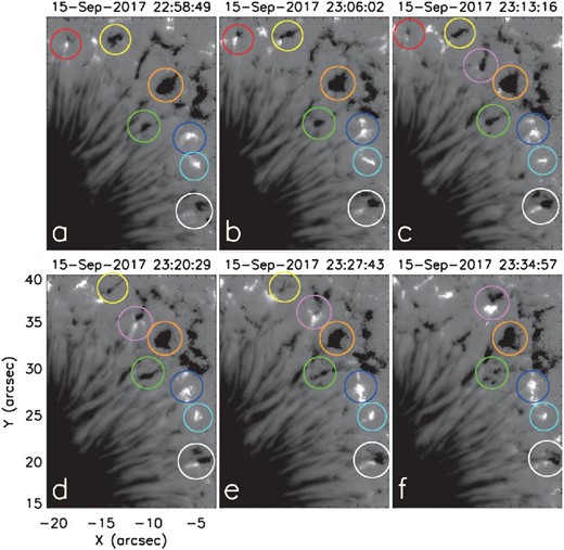
Line-of-sight magnetic field maps of the upper right quarter of a sunspot penumbra, including its surrounding moat region, observed by SOT-SP in Normal Map mode, thus having a pixel size of |${0{^{\prime \prime }_{.}}16}$|. The evolution of eight moving magnetic features are outlined by circles, each in a different color: red (panels a–c), yellow (panels a–e), orange (panels a–f), violet (panels c–f), green (panels a–f), blue (panels a–c), cyan (panels a–f), and ivory (panels a–f). The SP data used in this figure were inverted at the Community Spectropolarimetric Analysis Center 〈http://www2.hao.ucar.edu/csac〉. (Color online)
MMFs are proposed to play a crucial role in the decay of sunspots (Harvey & Harvey 1973; Martínez Pillet 2002; Hagenaar & Shine 2005). Consistent with the results of Hagenaar and Shine (2005), using Hinode/SOT data Kubo et al. (2008a, 2008b) showed that in decaying sunspots the rate of the loss of magnetic flux (8 × 10¹⁵ Mx s−1) in sunspots is very similar to the rate of the magnetic flux carried outwards by MMFs, thus taking several weeks for a sunspot of 1022 Mx to completely decay. Kubo et al. (2008a) also showed that positive and negative polarities balance each other in the moat region, suggesting that most of the sunspot flux is transported to the moat region and then outward by MMFs, and then removed by flux cancelation in the network regions. The rate of flux transport by moat flows is consistent with that found in recent MHD simulations of Rempel and Cheung (2014) and Rempel (2015).
Sunspot formation
The formation of sunspots, being a subsurface process (Parker 1955), remains observationally more poorly understood than their decay. Sunspots form as a result of the coalescence of small emerging magnetic elements (Zwaan 1985). In the MHD simulations of Cheung et al. (2010), Stein and Nordlund (2012), and Rempel and Cheung (2014), flux emergence in the form of fragmented flux tubes (caused by subsurface convection) consistently coalesce by horizontal inflow to make sunspots.
Much observational work has been devoted to penumbra formation. After a critical magnetic flux for an umbra is reached, any new flux joining the spot probably contributes to the formation of a penumbra (Schlichenmaier et al. 2010b). Using Hinode data, Shimizu, Ichimoto, and Suematsu (2012) found that an annular feature in Ca ii H in the form of a magnetic canopy surrounding the umbra in the chromosphere plays a role in the formation of penumbrae, thus proposing that knowledge of the chromospheric magnetic field is essential in understanding the formation mechanism of sunspot penumbrae. Kitai, Watanabe, and Otsuji (2014) concluded, again by using Hinode data, that a penumbra can form in a few different ways, e.g., by active accumulation of magnetic flux, or by a rapid emergence of new magnetic flux, or by the appearance of twisted or rotating magnetic tubes. The formation of a sunspot penumbra is still not fully understood, and apparently depends on various factors, e.g., field strength, field inclination, size, or amount of flux (Leka & Skumanich 1998; Rieutord et al. 2010; Rezaei et al. 2012; Kitai et al. 2014; Jurčák et al. 2015, 2017; Murabito et al. 2016, 2017).
7.1.5 Summary and future prospects
Sunspot physics has seen a major revolution in the first decade of the Hinode era. Unprecedented observations of sunspots by Hinode/SOT have revealed or clarified several small-scale aspects of sunspots, especially umbral dots and light bridges in the umbra, filaments, spines, and jets in the penumbra, field gradient inversions in the inner penumbra, MMFs, and peripheral downflows in the outer penumbra.
Hinode has solved several of the open questions that existed before the Hinode era. Some of the most striking discoveries are umbral dots having dark lanes, and magnetoconvective flows in UDs with the balanced mass-flux showing striking similarities with MHD models, granular light bridges having field-free regions, the internal structure of penumbral filaments, spines and filaments being the only components in the penumbra, MMFs being compatible with the idea of them being responsible for sunspot decay. The most striking new results are for the sunspot penumbra. Penumbral filaments are found to be elongated magnetized convective cells (Tiwari et al. 2013), qualitatively supporting recent MHD simulations (Rempel 2012). Several small-scale features were found to be part of penumbral filaments, e.g., penumbral grains were found to be the heads of filaments. Penumbral spines were observed to be a true outward extension of the umbral field. Sunspot penumbrae are formed entirely of spines and filaments (Tiwari et al. 2015).
Some enduring controversies about the complex penumbral structure, e.g., whether strands of more vertical field (spines) are warmer or cooler than strands of more horizontal field, whether the Evershed flow mainly takes place in dark or bright penumbral strands or there is no correlation between flow and brightness, whether more horizontal fields are found in darker or brighter penumbral regions, etc. [see Solanki (2003) for details], have been resolved by uncovering the fact that spines and parts of filaments have some properties in common (Tiwari et al. 2013). A few of the unexpected discoveries about sunspots using Hinode/SOT data include the magnetic field at the tails of penumbral filaments being stronger than that in the heads of penumbral filaments by 1–2 kG (Tiwari et al. 2013), the strongest magnetic field in many sunspots being found not in dark sunspot umbrae but rather often in light bridges (Okamoto & Sakurai 2018) or at the periphery of sunspots (van Noort et al. 2013).
Now we briefly mention some of the problems that should be addressed in the future using future-generation telescopes, e.g., DKIST and SOLAR-C_EUVST.
Concentrated downflows (with an opposite-polarity magnetic field to the umbra) surrounding umbral dots are expected from MHD simulations but have not been detected so far, probably because of the insufficient spatial resolution of currently available magnetic field data. The absence of such concentrated downflows and opposite-polarity field in higher-resolution data would challenge present MHD simulations.
Because of the limited temporal cadence of spectro-polarimetric data from Hinode, the lifetime of several small-scale features (e.g., penumbral filaments) remains poorly estimated. Further, how penumbral filaments form, evolve, and interact with spines remains to be explored. Filaments and spines could result from loading/unloading of convecting gas onto/from the spine field. Or, spines in a penumbra could be a result of overturning convection taking place between them. Once the vertical magnetic field is sufficiently weak and the field is sufficiently inclined, a sub-surface convective instability within the sunspot can perhaps take place to form a penumbral filament. To address the above, we need to follow a penumbra of decent size in higher temporal and spatial resolution spectro-polarimetric data for a couple of hours or more. Probably the formation mechanism of filaments and their interaction with spines also hold the answer to the formation mechanism of penumbral jets and bright dots, which may contribute to coronal heating above sunspots (Tiwari et al. 2016; Alpert et al. 2016).
Multi-height spectropolarimetric data are needed to provide a 3D picture of sunspots. A recent study by Joshi et al. (2016) showed the presence of fine-scale magnetic structure in the azimuthal direction in the upper chromospheric layers of sunspot penumbrae consistent with that found in the photosphere, albeit with reduced amplitudes. Moreover, to understand the force balance in sunspots and their equilibrium (e.g., Venkatakrishnan & Tiwari 2010; Puschmann et al. 2010; Tiwari 2012), we need to develop a technique to accurately estimate the geometrical heights of different small-scale features in sunspots.
7.2 Coronal jets
Coronal jets are common in all solar regions. Those in coronal hole and quiet-Sun regions can have some differences (perhaps only apparent differences) from those in active regions (ARs). We will discuss jets in ARs in more detail below. First, we will give a brief overview of observations and theoretical ideas of coronal jets in general. See Innes et al. (2016) and Raouafi et al. (2016) for other recent reviews. We will not include discussion of chromospheric jets.
7.2.1 Overview of coronal jet observations
Solar coronal jets are features seen at coronal wavelengths that grow out of the lower solar atmosphere, and reach long extents compared to their widths. They were seen in images from space-based telescopes launched in the 1970s. Most jets have a transient lifetime of only ∼10 min, and hence they were only observed and studied in detail from the time of the Yohkoh mission, launched in 1991.
Yohkoh observed jets in X-rays with its SXT (Tsuneta et al. 1991), which had 2|${^{\prime\prime}_{.}}$|5 pixel−1 resolution and variable cadence, with the highest being ∼20 s. It had a variable FOV, being capable of observing the full solar disk at reduced resolution and cadence, and smaller areas with higher cadence and resolution. Shibata et al. (1992) reported the first detailed SXT jet observations. In a statistical study of 100 X-ray jets, Shimojo et al. (1996) found that 68% of the jets occurred in the vicinity of ARs, but they also saw them in quiet Sun and coronal holes. They found average maximum lengths of ∼1.5 × 10⁴ km and velocities of ∼200 km s−1, with the values spanning a large range. They found most jets to have lifetimes of several 100 s to a few 1000 s, but they reported that the distribution of lifetimes extended out with a power-law distribution to many hours. Shimojo and Shibata (2000) found a selection of jets to have temperatures of 3 MK–8 MK (average 5.6 MK). These early studies also showed that jets have bright bases, often with a bright point off to one side of the base.
Subsequently, jets were also well observed in EUV, with SOHO/EIT (Delaboudinière et al. 1995; 2|${^{\prime\prime}_{.}}$|5 pixel−1, typically 12 min cadence), STEREO/SECCHI-EUVI (Wuelser et al. 2004; 1|${^{\prime\prime}_{.}}$|6 pixel−1, 1.5 min), and TRACE (Handy et al. 1999; 0|${^{\prime\prime}_{.}}$|1 pixel−1, 3–30 s). EIT and EUVI have full-Sun FOVs, while that of TRACE was only ∼8|${^{\prime}_{.}}$|5 square. As a consequence, observations of jets with these instruments were somewhat limited due to the time cadences for EIT and EUVI and the limited FOV for TRACE. Nonetheless, these studies yielded important jet results. For example, Wang et al. (1998), combining SOHO/EIT and LASCO images, found that EUV jets were the source of narrow white-light jets. Patsourakos et al. (2008) found clear helical structure in jets in EUVI images, and Alexander and Fletcher (1999) saw in high-resolution TRACE images a mixture of hot and cold material in jets, and evidence that the jets were rotating. See reviews by Nisticò et al. (2009) and Raouafi et al. (2016) for more details of jet observations with these instruments.
The next big step in jet observations occurred with the launch of the Hinode satellite, which gave us a fresh view of X-ray jets with its XRT, which has ∼1″ pixel−1 resolution and a maximum cadence of 10 s (many jet studies use XRT observing runs with cadence ∼1 min). As with SXT, it is capable of full-Sun observations but typically uses a reduced FOV for observing jets with higher resolution and cadence. XRT observes in X-rays with a variety of filters, with those sensitive to “softer” (sensitive to relatively cool plasmas of T ∼ 1 MK) X-rays, such as Ti-poly, C-poly, Al-mesh, and Al-poly, being the most useful for non-AR jet observations, while somewhat “harder” filters like Be-thin also show AR jets well. (We will not focus in detail on observations of jets with Hinode’s EIS and SOT instruments here.)
With XRT, Cirtain et al. (2007) found that X-ray jets are plentiful in polar coronal holes. Savcheva et al. (2007) measured the properties of XRT-observed polar jets, finding that they occur at a rate of ∼60 d−1 in the two polar coronal holes. They further found the jets to have, on average, outward velocities of 160 km s−1, maximum heights of 50000 km, widths of 8000 km, and lifetimes of 10 min. They found two distinct outward velocities: one of 160 km s−1, which is near the sound speed, and a second, faster, component of ∼800 km s−1, close to the expected Alfvén speed, providing evidence that Alfvén waves are transmitted into the corona. They also found the jets to have transverse velocities of 0–35 km s−1. See Raouafi et al. (2016) for further discussion of these waves and motions.
It is interesting that studies reported many more X-ray jets in polar coronal holes in XRT images than in SXT images. In part this may be a consequence of the observing sequences (time cadence, FOV, etc.) selected for studies with the respective instruments. Another factor, however, could be that XRT sees softer X-rays than did SXT, and therefore is able to detect cooler X-ray emissions. The temperatures of the spires of XRT-observed jets in polar coronal holes are ∼1.5–2.0 MK (Pucci et al. 2013; Paraschiv et al. 2015; Mulay et al. 2017), which are temperatures to which XRT has high sensitivity in its softer channels; this is much cooler than the ∼5.6 MK jet temperatures of the SXT-observed jets. At least a few polar jets, however, were in fact observed with SXT (Koutchmy et al. 1997).
Just as XRT revolutionized X-ray jet observations, AIA on SDO (Lemen et al. 2012) vastly improved jet observations in the EUV, with seven bands (304 Å, 171 Å, 193 Å, 211 Å, 131 Å, 94 Å, 335 Å), 0|${^{\prime\prime}_{.}}$|6 pixels, and 12 s cadence in the EUV channels. Another SDO instrument critical to jet studies is HMI, which takes line-of-sight photospheric magnetograms at 45 s cadence using 0|${^{\prime\prime}_{.}}$|5 pixels. Both AIA and HMI have full-Sun FOVs. We will discuss some of the XRT and SDO contributions to jet studies below. Most recently, IRIS has contributed to studies of jets (e.g., Cheung et al. 2015).
7.2.2 Ideas for the origin of coronal jets
Jets can occur in complex magnetic environments, and a natural suggestion was that they formed when newly emerging flux undergoes magnetic reconnection with the ambient coronal magnetic field. Shibata et al. (1992) made this suggestion, and a large number of numerical simulations based on (or inspired by) this idea result in features that look like jets (Yokoyama & Shibata 1995; Nishizuka et al. 2008; Archontis & Hood 2013; Moreno-Insertis & Galsgaard 2013; Fang et al. 2014). In this “emerging flux” idea, the base bright point of the jet originated from when the emerging flux underwent interchange reconnection with the ambient field; a resulting compact loop from that reconnection, it was suggested, produced the commonly observed bright point at the edge of the base of the jet, and the jet material flowed out along field lines newly opened by that reconnection.
Another view of the origin of coronal jets, a view not based on the emerging-flux idea, was suggested by Sterling et al. (2015). An earlier study (Adams et al. 2014) showed that an on-disk jet appeared to form from the eruption of a small-scale filament. Others had also seen jets resulting from flare-type eruptions or small-filament eruptions in some cases (e.g., Moore et al. 1977; Nisticò et al. 2009; Raouafi et al. 2010; Shen et al. 2012; Huang et al. 2012). Sterling et al. (2015) observed 20 random polar coronal hole jets in both X-rays from XRT and in multiple EUV channels with AIA. They found that all of the jets resulted from eruptions of miniature erupting filaments, or minifilaments. These eruptions looked essentially the same as large-scale filament eruptions, except for the smaller size (∼8000 km for the minifilaments, while typical filaments have lengths of several × 104 km).
They explained their observations with the idea shown schematically in figure 26d–26f. The magnetic setup is that of a minority polarity surrounded by a majority polarity in the jet region (also called an “anemone” region; Shibata et al. 2007). The pre-eruption minifilament sits in a compact sheared-field bipole on a neutral line on one side of the minority polarity area; so in cross-section it is a double bipole, with one side (containing the minifilament in the sheared field) more compact than the other. When that minifilament erupts, it first moves over the top of the neighboring bipole, and then erupts outward in the spire. The spire results when the field enveloping the erupting minifilament reconnects with the ambient coronal field, and the bright point at the jet’s base edge, which Sterling et al. (2015) called a jet bright point, or JBP, forms when the field beneath the erupting minifilament field undergoes reconnection; this reconnection is identical to that occurring beneath erupting large-scale filaments that produces flares, according to the standard model for solar eruptions/flares (Shibata & Magara 2011). Thus, in this view the JBP beneath the erupting minifilament is analogous to a solar flare beneath an erupting large-scale filament.
![(a)–(c) Hinode/XRT Be-thin filter images at indicated times of a jet from AR 12259, with an HMI magnetogram from 2015 January 14, 14:20 39 UT, overlaid. In the magnetogram, green and blue represent positive and negative polarities, respectively, and the contours are at 50, 100, and 750 G. See Sterling et al. (2017) for more details and videos of this event. (d)–(f) Schematic showing the minifilament eruption coronal jet mechanism suggested by Sterling et al. (2015). [This version of the schematic is adopted from Sterling et al. (2016) by permission of the AAS.] Initially, (d) a cool (chromosphere/transition-region temperature) minifilament (blue circle) resides in a bipole on a magnetic neutral line (A)–(B), adjacent to a larger bipole (B)–(C). Black/red lines represent magnetic field lines before/after reconnection. As the minifilament erupts (e) it encounters the opposite-polarity field on the far side of the larger bipole, with resulting reconnections (red Xs) making a new open field along which the jet spire forms. Also, loop (A)–(B) brightens, forming a jet (or jet-base) bright point; this occurs due to flare-type reconnection occurring among the legs of the erupting minifilament field. As the eruption continues, (f) the spire broadens, and the large bipole (B)–(C) brightens and grows due to the addition of reconnection-formed loops. The long arrows between (d) and (a) show approximate correspondences between the schematic and the observed AR jet. This schematic picture was derived from coronal hole jet observations; the situation in ARs seems similar, but more complex, perhaps due to the more complex and stronger, more rapidly evolving fields of ARs compared to other regions (see text). In addition, in 3D the reconnections would be more complex than illustrated here. (Color online)](https://oup.silverchair-cdn.com/oup/backfile/Content_public/Journal/pasj/71/5/10.1093_pasj_psz084/2/m_pasj_71_5_r1_f19.jpeg?Expires=1749038438&Signature=GCXvHepUXUhW2gME3APpDQXzQTJX89UuVS~pJDa3s3rud3szItHyOrterhj~SPgB6sEaNkK6-Qp-Y7e2EokZftd9mrg1TfiJ1EjCo5wkEJnmJWGPbyUPi8jtprphcZRKU7IHKqiMvV-r~ZdBQ5mrVI7EGmP85Mk8cnufrvWKPX3xXYp5k5mYuzi9dTE~zqVTnO5y2zA2Tp3wjKiBxkJoBZBbh5gIEQjd3ZOumLPM1XGvdVsy0ykDueRf85rl5EQGIA~VxfbSqz~e1Wp-WioIjpDIMHowHao0x5hPp-Rk5Y7vM720SobtNA4kKu9iOYtwMoyXgK-zaze~oTAYmIRKtQ__&Key-Pair-Id=APKAIE5G5CRDK6RD3PGA)
(a)–(c) Hinode/XRT Be-thin filter images at indicated times of a jet from AR 12259, with an HMI magnetogram from 2015 January 14, 14:20 39 UT, overlaid. In the magnetogram, green and blue represent positive and negative polarities, respectively, and the contours are at 50, 100, and 750 G. See Sterling et al. (2017) for more details and videos of this event. (d)–(f) Schematic showing the minifilament eruption coronal jet mechanism suggested by Sterling et al. (2015). [This version of the schematic is adopted from Sterling et al. (2016) by permission of the AAS.] Initially, (d) a cool (chromosphere/transition-region temperature) minifilament (blue circle) resides in a bipole on a magnetic neutral line (A)–(B), adjacent to a larger bipole (B)–(C). Black/red lines represent magnetic field lines before/after reconnection. As the minifilament erupts (e) it encounters the opposite-polarity field on the far side of the larger bipole, with resulting reconnections (red Xs) making a new open field along which the jet spire forms. Also, loop (A)–(B) brightens, forming a jet (or jet-base) bright point; this occurs due to flare-type reconnection occurring among the legs of the erupting minifilament field. As the eruption continues, (f) the spire broadens, and the large bipole (B)–(C) brightens and grows due to the addition of reconnection-formed loops. The long arrows between (d) and (a) show approximate correspondences between the schematic and the observed AR jet. This schematic picture was derived from coronal hole jet observations; the situation in ARs seems similar, but more complex, perhaps due to the more complex and stronger, more rapidly evolving fields of ARs compared to other regions (see text). In addition, in 3D the reconnections would be more complex than illustrated here. (Color online)
This minifilament eruption viewpoint can also address the twisting motions frequently reported in coronal jets (e.g., Pike & Mason 1998; Patsourakos et al. 2008; Raouafi et al. 2010; Shen et al. 2011; Chen et al. 2012; Hong et al. 2013; Schmieder et al. 2013b; Li et al. 2015b; Moore et al. 2015). If the pre-eruption minifilament field already contains twist, that twist can be released as the erupting field reconnects with the ambient coronal field, imparting its twist onto that field (see Shibata & Uchida 1986).
By examining over 50 jets in polar coronal holes as seen by XRT, Moore et al. (2010, 2013) found that X-ray jets tended to appear as one of two types, which they called “standard jets” and “blowout jets.” These terms describe the morphology of the jets as seen in X-rays: For standard jets, the jet spire remains narrow (compared to the size of its base) over the lifetime of the jet, and the JBP is generally off to one side of the base. For blowout jets, the spire starts off narrow, but expands until its width is comparable to the size of the base region, and the base interior also usually brightens to be about as bright as or even brighter than the JBP. Blowout jets were so named because they have similarities with filament eruptions. Standard jets were so named because, at that time, the authors thought that the narrow jets were “standard” cases of jets following the emerging-flux model predictions. That group of authors has, however, now come to believe that instead of resulting from the emerging-flux model, essentially all jets, both blowout and standard, result from minifilament eruptions (Sterling et al. 2015; Moore et al. 2018): the standard jets have narrow spires in X-rays because the minifilament eruption either fails to escape the base region, analogous to confined solar eruptions (e.g., Moore et al. 2001), or perhaps escapes but the eruption is very weak.
Moreover, on-disk studies of quiet-Sun and coronal hole jets unambiguously show that jets frequently result from flux cancelation rather than emergence. Several earlier single-event (or small number of events) studies showed this (e.g., Hong et al. 2011; Huang et al. 2012; Adams et al. 2014; Young & Muglach 2014a, 2014b). More recently, Panesar et al. (2016b, 2018) argued that flux cancelation occurs in all of the quiet-Sun and coronal hole jets they studied (23 in total); some of their jets occurred with flux cancelation in conjunction with flux emergence, but in those cases the jet originated from where one pole of the emerging field canceled with the surrounding field, and so cancelation seems to be the critical factor in all of their events. Kumar et al. (2018) presented one jet that they argued was caused by shearing fields, without substantial cancelation or emergence. Finally, Panesar, Sterling, and Moore (2017) presented evidence that, for 10 quiet-Sun jets that they studied, the minifilaments (that erupted to produce the jets) themselves formed at sites of flux cancelation.
Recently, the minifilament eruption model for jets has been simulated by Wyper, Antiochos, and DeVore (2017) and Wyper, DeVore, and Antiochos (2018), who refer to the process as a “breakout model” for jets.
7.2.3 Coronal jets in active regions
While we expect that AR jets are the same as quiet-Sun and coronal hole jets, in practice they can have some morphological differences. Perhaps all of these differences can be explained by the stronger and more complex magnetic field of the region in which they are generated; further studies will have to verify whether this is the case, or if instead there are some intrinsic differences between AR jets and jets in quieter regions. In particular, AR jets do not show erupting minifilaments in EUV as commonly (or at least not as clearly) as in coronal hole and quiet-Sun jets. Here we present some results mainly from recent AR jet studies, including the question of whether erupting minifilaments cause them too.
As mentioned above, most of the Yohkoh/SXT-observed X-ray jets occurred in ARs, and so the jet properties given by, e.g., Shimojo et al. (1996) and Shimojo and Shibata (2000), are skewed toward AR jets. Others, including Kim et al. (2007) and Mulay et al. (2016), have also studied properties of AR jets. There is little doubt that AR jets tend to be more energetic than coronal hole jets. Pucci et al. (2013) found that two polar coronal hole jets had a total energy of ∼1026–1027 erg, while Shimojo and Shibata (2000) found jets (probably mainly AR jets) in their study to have thermal energies of ∼1027–1029 erg. Also, Sterling et al. (2015) found all of their coronal hole X-ray jets to be seen well only in relatively cool AIA channels: 304, 171, 193, and/or 211 Å. AR X-ray jets, on the other hand, are generally easily visible in hotter AIA channels also, such as 94 Å (Sterling et al. 2016, 2017), suggesting that they contain larger amounts of hotter plasmas than do coronal hole jets (and presumably most quiet-Sun jets also).
In ARs, relatively strong fluxes of both polarities can be plentiful and the magnetic evolution very fast. This often leads to flux emergence and cancelation occurring concurrently at jetting sites (e.g., Shimojo et al. 1998; Shen et al. 2012; Li et al. 2015a; Panesar et al. 2016a; Sterling et al. 2016), with some events showing only cancelation (e.g., Chifor et al. 2008a, 2008b). Sterling et al. (2017) argued that, even in the mixed emerging and canceling conditions of ARs, cancelation appeared to be the primary trigger of jets. However, Mulay et al. (2016) argued that 70% of the 20 jets they studied included flux cancelation, and 30% occurred with flux emergence alone. Thus, more investigation is needed into the question of what triggers jets to erupt.
Sterling et al. (2016) considered in detail whether the minifilament eruption mechanism could explain a set of coronal jets they observed in an AR. They found that all of those jets occurred at the location of magnetic neutral lines, usually undergoing cancelation, but in some cases showing both emergence and cancelation. In two jets, they saw clear evidence for a minifilament eruption leading to a surge-like jet. Hinode data were not available for that study, but in GOES/SXI X-ray images those two jets were weak or invisible. Many other jets of that AR, however, showed strong X-ray signatures, and although their magnetic geometry agreed with that expected in the case of the minifilament eruption mechanism, erupting minifilaments themselves were not apparent for those cases. Those jets were more rapidly developing and explosive (“violent”) than the ones that produced the surges with weak X-ray signatures.
Sterling et al. (2017) explored such violent jets in a different AR. In this case the jets had strong X-ray signatures (this time observed with XRT; see figure 26). Again, the magnetic setup for the jets was consistent with expectations from the minifilament eruption scenario, and this time the jets clearly originated from locations of flux cancelation, with the episodes of jetting continuing until a minority flux patch was completely consumed by the cancelation. In some cases they could identify erupting minifilaments causing the jets, but they observed that the minifilaments were very thin “strands,” having cross-sections of width less than about 2|${^{\prime \prime }}$|; this is about a factor of two thinner than the erupting minifilaments seen in polar coronal holes by Sterling et al. (2015), the on-disk jet-producing erupting minifilaments of Panesar et al. (2016b), or the surge-like eruptions of the AR jets of Sterling et al. (2016). Schmieder et al. (2013b) also reported observing strands or “threads” in an AR jet. Another difference between some AR jets and many jets in other regions is that the strongest base brightening was often the lobe adjacent to the erupting minifilament, rather than the location from which the minifilament emanated. Whether these differences between many AR jets and many non-AR jets can be fully explained with the minifilament eruption scenario, or whether a different mechanism is responsible, are questions that require further study.
Other investigations using Hinode data to study AR jets include Nitta et al. (2008), who found an AR jet to be the source of an 3He-rich solar energetic particle (SEP) event; He et al. (2010), who examined the AR jet–solar wind connection; and Lee et al. (2013), who observed helical motions, multi-thermal plasmas, and other features with all three Hinode instruments in a limb AR jet. Chifor et al. (2008b), Nishizuka and Hara (2011), Yang et al. (2011), Matsui et al. (2012), and Shelton, Harra, and Green (2015) studied Hinode/EIS spectroscopic aspects of AR jets. Zhelyazkov, Chandra, and Srivastava (2016) performed an MHD instability analysis of a jet observed by Chifor et al. (2008a). Cheung et al. (2015) studied recurrent AR jets and modeled them with data-driven simulations, showing that emerging flux can supply the twist needed for recurrent helical jet formation.
7.2.4 Additional comments
This review emphasizes the role of minifilament eruptions and flux cancelation in jets, in part as a result of the author of this section (A.C. Sterling) having been involved in studies indicating that these factors are important in jets. More general presentations are available in the Innes et al. (2016) and Raouafi et al. (2016) reviews mentioned at the start. At the time of those earlier reviews, however, the importance of minifilament eruptions and flux cancelation to jets was just starting to be recognized; still, Innes et al. (2016) did note many important examples of cancelation. It is unmistakable that recent observations (mainly in coronal holes and quiet Sun) show that many jets do indeed result from minifilament eruptions, frequently triggered by magnetic flux cancelation. Some jets, however, do occur without obvious minifilament eruptions or cancelation, and these cannot be ignored. Future observational studies should investigate what fraction of jets result from minifilament eruptions and flux cancelation processes, and what percentage might result from other processes such as shearing fields or flux emergence. Studies should also confirm whether the physical processes occurring in AR jets are the same as those in quiet-Sun and coronal hole jets. If most jets result from minifilament eruptions, this would be consistent with the basic idea presented in Shibata (1999) that coronal jets are scaled-down versions of large eruptions.
There are many other interesting topics regarding jets not discussed here, e.g., evaporation flows (Shimojo et al. 2001; Miyagoshi & Yokoyama 2004), whether jets are magnetically or evaporation driven (Chifor et al. 2008b; Matsui et al. 2012), the role of Alfvén waves (Nishizuka et al. 2008), mixture of hot and cool material in jets (Yokoyama & Shibata 1995; Canfield et al. 1996), and other topics. In many of these works, however, it is assumed that jets are formed via the emerging-flux mechanism. Thus, it is important for future studies to determine whether there is direct observational evidence that a substantial fraction of jets results primarily from the emerging-flux mechanism. If such evidence is not found, then these ideas should be reconsidered in light of the updated observations.
7.3 Emerging flux
7.3.1 Introduction
It has been widely thought that ARs are produced through flux emergence, the transportation of dynamo-generated magnetic flux from the convection zone to the surface of the Sun (Parker 1955). In newly emerging flux regions, different magnetic structures of various size scales are observed. For instance, in the magnetograms of figure 27, which shows the time evolution of AR 11130 from its earliest stage, one may find that the AR appears as tiny magnetic elements of positive and negative polarities. These elements merge together to form larger structures, i.e., pores (radius 0.7–1.8 × 10³ km) and sunspots (radius 4–28 × 103 km)—values adopted from Zwaan (1987). Typically, as a whole, ARs show a “cell division”-like separation of both polarities and develop into a bipolar configuration (third panel). The growth of magnetic structures is clearly seen in the power spectrum (bottom panel). Here, the slope becomes steeper with time, indicating that the larger structures are transported to the surface from below in the later phase and/or they are gradually formed around the surface via interactions between magnetic elements (i.e., inverse cascade).
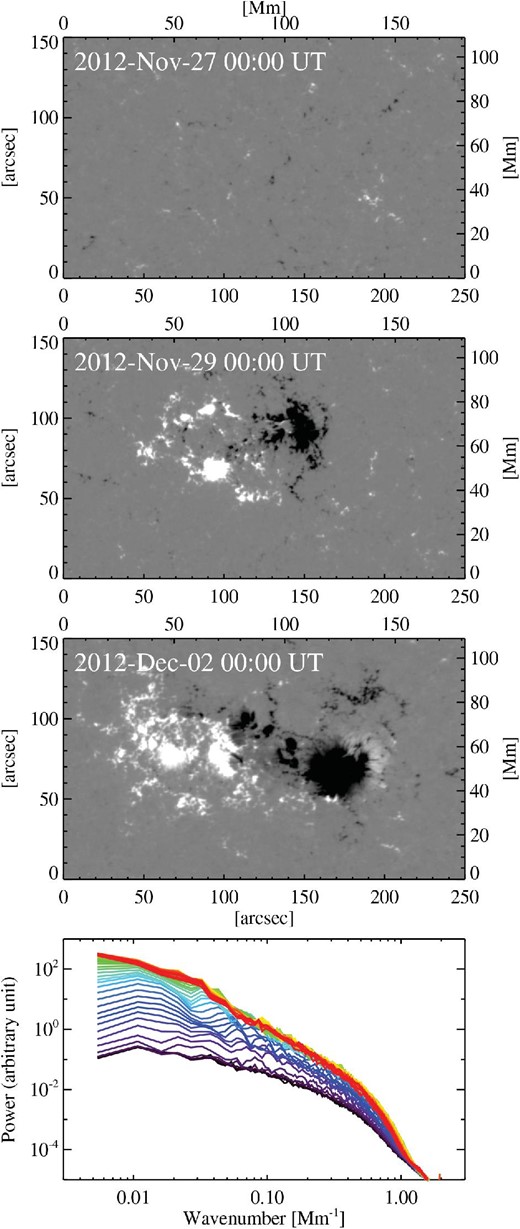
Top to third panels: Sequential magnetograms showing the emergence and formation of AR 11130 obtained by SDO/HMI. Bottom panel: Time evolution of the power spectrum produced from the sequential magnetograms. Color varies with time from purple (2012-Nov-27 00:00 UT) to red (2012-Dec-02 00:00 UT). Adapted from Toriumi, Hayashi, and Yokoyama (2014) by permission of the AAS. (Color online)
Over the course of their evolution, emerging flux regions produce a number of activity phenomena including miniature energy-releasing events as represented by Ellerman bombs, plasma ejections such as Hα surges and X-ray jets, and catastrophic eruptions, i.e., flares and CMEs. In this section we review the Hinode observations of flux emergence and some related activity phenomena in the earliest phase in the AR development.
7.3.2 Before the Sun rises
Before the launch of Hinode, when the mission was still called SOLAR-B, a number of meetings were held to discuss science objectives and possible observation proposals. Motivated by space observations (e.g., Yohkoh, SOHO, and TRACE), high-resolution ground-based observations (e.g., SST), and the state-of-the-art 3D numerical simulations realized in the 1990s and early 2000s, various topics were actively proposed. We introduce here several science targets discussed in one such conference, the Sixth SOLAR-B Science Meeting, held in Kyoto in 2005 November, i.e., just one year before the Hinode launch.
The first topic was flux emergence and the resultant magnetic reconnection with ambient fields. On the theoretical side, Moreno-Insertis (2007) and Isobe et al. (2007a) showed MHD simulations of flux emergence that introduced pre-existing coronal fields (Yokoyama & Shibata 1995; Archontis et al. 2005; Isobe et al. 2005) and emphasized the importance of observing the magnetic reconnection between emerging and pre-existing magnetic systems. They suggested, for example, that EIS will observe the current layer that forms between the two magnetic systems and the flow fields around the reconnection region (i.e., inflows and outflows). Kurokawa et al. (2007) introduced the observations of Hα surges emanating from emerging flux regions. They pointed out that the ejections will be caused by magnetic reconnection occurring in the lower atmosphere between the emerging field and the pre-existing field of opposite polarities (Yoshimura et al. 2003). They expected that such magnetic evolutions will be observed by SOT.
Another observation target was the coronal evolution in response to flux emergence. Yoshimura (2007) compared the photospheric magnetic flux (SOHO/MDI) and the coronal brightness in EUV (TRACE), and found that the EUV brightness increased in pace with the enhancement of the magnetic flux, which indicated that the magnetic fields continuously heated the corona. Such dynamic evolutions may be revealed with the combination of Hinode’s three instruments.
Scharmer et al. (2007), Stein, Benson, and Nordlund (2007), and Title (2007) discussed the importance of magnetoconvection from both theoretical and observational aspects. For example, radiative MHD simulation of flux tube emergence by Cheung, Schüssler, and Moreno-Insertis (2005) showed that bright and elongated granular cells are formed as the flux appears at the photosphere. Because the emerged horizontal fields guide the plasma flows, the granular cells become elongated and aligned to the direction of the magnetic fields. The close coupling of magnetic field and convection, seen not only in the quiet Sun but also in the earliest phase of AR evolution, was expected to be a favorable target for the Hinode mission, as stated by Lites (2007) in the summary review of the conference.
7.3.3 Hinode era
Since being launched successfully in 2006 September, Hinode has conducted numerous observations of a variety of solar phenomena. However, because of the limited FOV, especially of SOT, it has always been challenging to detect AR-scale flux emergence events. Also, in the first few years of the Hinode mission the Sun was at the cycle minimum and thus there were not many ARs. However, these constraints led to the successful detection of granular-sized emergence events.
Centeno et al. (2007) focused on the quiet-Sun inter-network region using Hinode/SOT-SP and found that as the granular cell turned over, positive and negative polarities that sandwiched the horizontal flux became separated (figure 28a). The eventual disappearance of the horizontal flux (final panel) indicated the emergence of an Ω-shaped loop. This is a perfect example of an emerging magnetic field coupled with or driven by local granulation, which was predicted by the numerical simulations. Also, Guglielmino et al. (2008) detected the chromospheric brightenings in Ca ii H in association with small-scale emergence, while Martínez González et al. (2010) estimated the emergence speed to be ∼3 km s−1 (photosphere) to ∼12 km s−1 (chromosphere). These are the representative observations of granular-scale emergence and its impact on the upper atmosphere (Isobe et al. 2008). For further descriptions of the quiet-Sun magnetism, readers are referred to subsections 3.1 and 3.2.
![(a) Granular-scale flux emergence event observed by Hinode/SOT-SP [Centeno et al. (2007), reproduced by permission of the AAS]. The background shows the integrated continuum intensity, while the red, green, and orange contours represent positive circular, negative circular, and linear net polarization signals, respectively. The images are separated by 125 s. (b) Hinode/SOT-NFI Stokes V images showing the emergence and evolution of AR 10926 [Magara (2008), reproduced by permission of the AAS]. (c) Hinode/EIS Fe xii intensity (reversed contrast) and Doppler velocity (saturating at ±50 km s−1) of AR 10926 (Harra et al. 2010). The FOV is shown as a white box in the middle panel of panel (b). Arrows indicate the blueshifted edge. (d) Frequency of flux emergence events of various scales against the flux content (Thornton & Parnell 2011). (e) Scatter plot of maximum total flux Φmax and mean flux growth rate 〈dΦ/dt〉 for 101 flux emergence events (Otsuji et al. 2011). (Color online)](https://oup.silverchair-cdn.com/oup/backfile/Content_public/Journal/pasj/71/5/10.1093_pasj_psz084/2/m_pasj_71_5_r1_f21.jpeg?Expires=1749038438&Signature=JsBd-MNVT8pUYuImdIcShbcDq~J8wDqPbakEezHfDmCca745Ig0pgi3YMw5~RXOFSdaakfWhGgb6Clafmf8Oe6Zk-a95yGJc~1R6-se4y2U0GKQAqSWlviKxMRdDXG-0hC8BwGETD6C9ivuJDUpr~Tda~5vHz1F92zQIIx6plIE7EWSJDGQLeYlbsq12bNRIVr4KVRwY8~h2bBYC9mML-RoBe81C5Agu2emlbnksoXTXYNumrdYqEq8lvVP6iFe8OS~SkRNoC3IR-0RwK4ouApG~WX5z8BIJx3RpUcqg5OX5fbf8eAh9A~BAzz1wrzmjEKeeROH9VJJ-nM0wnud6ww__&Key-Pair-Id=APKAIE5G5CRDK6RD3PGA)
(a) Granular-scale flux emergence event observed by Hinode/SOT-SP [Centeno et al. (2007), reproduced by permission of the AAS]. The background shows the integrated continuum intensity, while the red, green, and orange contours represent positive circular, negative circular, and linear net polarization signals, respectively. The images are separated by 125 s. (b) Hinode/SOT-NFI Stokes V images showing the emergence and evolution of AR 10926 [Magara (2008), reproduced by permission of the AAS]. (c) Hinode/EIS Fe xii intensity (reversed contrast) and Doppler velocity (saturating at ±50 km s−1) of AR 10926 (Harra et al. 2010). The FOV is shown as a white box in the middle panel of panel (b). Arrows indicate the blueshifted edge. (d) Frequency of flux emergence events of various scales against the flux content (Thornton & Parnell 2011). (e) Scatter plot of maximum total flux Φmax and mean flux growth rate 〈dΦ/dt〉 for 101 flux emergence events (Otsuji et al. 2011). (Color online)
From a theoretical point of view, one of the significant achievements in the Hinode era is the establishment of the “two-step emergence” model, in which the magnetic flux rising in the convection zone slows down due to the strong stratification and drastically deforms its shape in the lateral direction (pancaking), driving strong plasma outflows ahead (e.g., Cheung et al. 2010; Toriumi & Yokoyama 2010, 2011). Figure 29 presents a 3D simulation of a large-scale emergence. Here, the flux tube experiences a temporal deceleration and flattening before it expands into the photosphere and above. One of the most striking observational demonstrations of the two-step process is the Hinode and Hida observation by Otsuji et al. (2007, 2010). They found that the emerging flux first underwent a horizontal expansion in the photosphere at a speed of ∼3 km s−1, and then started rising into the chromosphere at ∼1 km s−1, later increasing to ∼2 km s−1. The clear consistency of the theory and observation symbolizes the success of the Hinode mission. In this period, the ascension, deceleration, and escaping outflows of the magnetic flux were also observed with other methodologies (e.g., Grigor’ev et al. 2007; Ilonidis et al. 2011; Toriumi et al. 2012, 2013b; Khlystova 2013), which further fostered our understanding of flux emergence.
![Numerical simulation and observation of the “two-step emergence” process. (a)–(d) Three-dimensional MHD simulation of a rising magnetic flux tube from the deeper convection zone (from −2 × 10⁴ km: H0 = 200 km, τ0 = 25 s, and B0 = 300 G), and (e) its height–time evolution [Toriumi and Yokoyama (2012), reproduced by permission of ESO]. Here, the rising flux tube decelerates and expands horizontally at the top convection zone [panels (b) and (c)] before it emerges into the photosphere and beyond. The horizontal expansion and second-step acceleratory emergence into the atmosphere was detected by Hinode and Hida Observatory. The schematic illustration of (f) summarizes the observed characteristics [Otsuji et al. (2010), reproduced by permission of OUP]. (Color online)](https://oup.silverchair-cdn.com/oup/backfile/Content_public/Journal/pasj/71/5/10.1093_pasj_psz084/2/m_pasj_71_5_r1_f22.jpeg?Expires=1749038438&Signature=VstTBnx5qSJdZ0fQupGjgqyeA~wRHOy8dI8uQOIn52XmbOMAT-iSQ7OYAKFUAvASsqg2xc2ajO~RbrRWM3WzoUbBkJnYG2ZhY2jT8faGALlJ0f6T2zAq4r2U5pe8Bp5AG9E5IRsclhLOnHP39dN2o8TU8ag0QHocv3Yn3zvk3~bisWZ4bwtN7HJ4~NyhGqLzAgczBsScFZnd4ZDHBWli1cCnLxKsLF2qC5qdhA1fzOM89yq5LCf8sgKB-kir7DCSyb4Q1ddy7kcUDC3x3TZOqbmayePdGbalZK15WmDd-Qcb3UR73V9~ffuIn2W-oQY5dIUF4buzfTTEr8ATXuxtDg__&Key-Pair-Id=APKAIE5G5CRDK6RD3PGA)
Numerical simulation and observation of the “two-step emergence” process. (a)–(d) Three-dimensional MHD simulation of a rising magnetic flux tube from the deeper convection zone (from −2 × 10⁴ km: H0 = 200 km, τ0 = 25 s, and B0 = 300 G), and (e) its height–time evolution [Toriumi and Yokoyama (2012), reproduced by permission of ESO]. Here, the rising flux tube decelerates and expands horizontally at the top convection zone [panels (b) and (c)] before it emerges into the photosphere and beyond. The horizontal expansion and second-step acceleratory emergence into the atmosphere was detected by Hinode and Hida Observatory. The schematic illustration of (f) summarizes the observed characteristics [Otsuji et al. (2010), reproduced by permission of OUP]. (Color online)
Chromospheric anemone jets observed near the limb by Shibata et al. (2007) indicated the possibility that the small-scale magnetic reconnection between the emerging flux and the pre-existing field occurs ubiquitously in the solar atmosphere. Multi-wavelength analysis of the reconnection was reported by Guglielmino et al. (2010). It was found that the small-scale emergence within an AR was associated with chromospheric, transition-region, and coronal brightenings as well as chromospheric surge ejections. With the support of magnetic field extrapolation, they revealed that the overall scenario is in line with the above mechanism; namely, the interaction between the emerging flux and the pre-existing ambient fields. A similar event was detected by collaborative observation with SOT and the New Solar Telescope (NST) of the Big Bear Solar Observatory (Yurchyshyn et al. 2010). It is now thought that jet ejections caused by emerging flux and ambient field occur at a wide range of scales (see subsection 7.2).
One of the earliest detections of AR-scale flux emergence events was given by Magara (2008). Figure 28b clearly shows that the fragmented magnetic elements merged to develop a large bipolar structure; see the scale difference from figure 28a. Such large-scale evolutions of emerging magnetic flux and the resultant spot motion are important for the build-up of the free magnetic energy and the supply of shear and helicity that are essential to the flare eruptions (e.g., Magara 2009). It is also believed that emerging flux can trigger flares and CMEs (e.g., Kusano et al. 2012). See section 8 for further details.
The atmospheric response to the photospheric flux evolution was also investigated. One of the earliest attempts was made by Hansteen et al. (2007), who used SOT and EIS to reveal that a dark dimming region appeared and expanded in He ii and Fe xii about 30 min after the flux emerges in the photosphere. Del Zanna (2008b) investigated the Doppler shift of coronal lines in AR 10926 (Magara 2008; figure 28b) and found that the blueshifts appeared in lower hot (3 MK) loops, which was ascribed to the continuous flux emergence. Harra et al. (2010) analyzed the same AR and detected the formation of coronal loops at the locations of newly emerging magnetic elements. They found blueshifts with enhanced intensities and line widths at the edges of the emerging flux region (figure 28c), which they interpreted as the onset of AR outflow that could contribute to the slow solar wind (Sakao et al. 2007). Further review of the coronal response to AR evolution is found in section 9.
Yet another topic that we should mention is the statistical investigations. Analyzing the high-cadence, high-resolution polarimetric imaging data of Hinode/SOT-NFI, Thornton and Parnell (2011) found that the frequency of flux emergence shows a power-law distribution over nearly seven orders of magnitude from AR-scale (1023 Mx) to granular-scale (1016 Mx) events (figure 28d). The obtained power-law index was less than −2, indicating that most of the newly supplied flux to the surface layer is from small-scale events and that the emergence rate is independent of the solar cycle. Otsuji et al. (2011) analyzed more than 100 events with total magnetic flux from 3 × 10¹⁷ to 3 × 10²¹ Mx and found that the maximum separation distance, flux growth rate, and mean separation speed of the bipoles showed power-law relations with the total flux (figure 28e). Applying the feature-tracking method to sequential magnetograms, Iida, Hagenaar, and Yokoyama (2012) detected flux emergence events or, more precisely, separating motions of positive and negative polarities. These Hinode observations clearly revealed the scale-free nature of magnetic flux emergence.
During the past ten years, numerical simulations of flux emergence have been extensively developed and become increasingly sophisticated, which allows more direct comparisons between modeling and Hinode observations. For example, Cheung et al. (2008) conducted flux emergence simulations that took into account the effect of radiative transfer and compared them with SOT observations. They successfully reproduced the observational characteristics in emerging flux regions, such as elongated granules and flux cancelation (Cheung et al. 2010; Rempel & Cheung 2014). With the help of simulations, Nishizuka et al. (2008) found that the chromospheric anemone jets (Shibata et al. 2007) can be explained by the scenario of emerging flux reconnecting with the ambient magnetic field (Yokoyama & Shibata 1995), while Murray et al. (2010) and Harra et al. (2012) proposed the possibility that the AR outflow is caused by the plasma compression and reconnection between the emerging flux and the pre-existing open flux.
7.3.4 Hinode, IRIS, and beyond
Launched in 2013 June, IRIS opened a new door to understanding the dynamics of the chromosphere and transition region (De Pontieu et al. 2014b). One of the primary science targets of IRIS was to reveal the transportation of magnetic fields through the lower atmosphere, i.e., flux emergence and its relation to various activity phenomena. Therefore, it is crucially important to simultaneously observe the detailed surface magnetic fields and the atmospheric dynamics, which can best be realized by coordinated campaigns by Hinode and IRIS. Although there have not been many published observational results of this kind, we introduce here one coordinated observation that clearly showed the connection between photospheric fields and atmospheric activity events in an emerging region (Toriumi et al. 2017).
The target emerging flux region appeared in the middle of AR 12401 on 2015 August 19. Figure 30 displays an overview of the region and a representative local energy-releasing event (Ca brightening). One may see from this figure that Ca brightenings were scattered over the entire region, which was overlaid by an arch filament system (Bruzek 1967) seen in the core of the Mg ii k line. The Ca brightenings were quite small (the brightest part being ≲1″). In the center of the region, they were mostly located at the polarity inversion lines between closely neighboring magnetic elements of the two polarities. Regarding the representative event, the photospheric vector magnetogram obtained by SOT-SP shows that the polarity inversion line had a dipped configuration (the so-called bald patch; Pariat et al. 2004). Above, in the chromosphere and the transition region, the UV spectra taken by IRIS were significantly enhanced and widened, and, especially for Si iv and C ii, the spectra had a positional dependence: they were redshifted on the disk-center side and blueshifted on the limb side (Peter et al. 2014; Vissers et al. 2015). The purple profile at the middle is long tailed, reaching ±100 km s−1. The Mg ii triplet was seen in emission, indicating a strong temperature enhancement in the lower chromosphere (>1500 K; Pereira et al. 2015; Vissers et al. 2015; Tian et al. 2016a).
![Emerging flux region in AR 12401 and a representative energy-releasing event detected simultaneously by Hinode and IRIS [reproduced from Toriumi et al. (2017) by permission of the AAS]. The top row shows the Hinode/SOT-SP circular polarization (CP) map and IRIS Mg ii k3 intensity map. The red contour shows the enhanced brightenings in SOT Ca ii H. The second row shows the AIA 1700 Å, IRIS 1400 Å slit-jaw image, SOT Ca ii H, and the SOT-SP CP map of the representative event indicated by a yellow arrow in the top left-hand panel. White contours delineate the enhanced Ca brightening, while the arrow shows the direction of the disk center. Yellow and turquoise dots indicate the concave-up and concave-down polarity inversion lines, respectively. The third and fourth rows show three IRIS UV spectra and SOT-SP Stokes V/I profiles. Three colors represent the three locations in the second row, black profiles are the quiet-Sun levels, and the vertical lines indicate the line centers. (Color online)](https://oup.silverchair-cdn.com/oup/backfile/Content_public/Journal/pasj/71/5/10.1093_pasj_psz084/2/m_pasj_71_5_r1_f24.jpeg?Expires=1749038438&Signature=FMWuvbThjiDUUFACcVa57fDX0gM1eWoRqHebXJcxWjg1vul8lozlaIGq8SEADKkR-w9XLWmMphBKtoMRDmoEoJ8VJbVsak-SJYq7RqnYDWVxsQdoOdqwhD-1sk2ctOrDqSONCxiWTcoPACcOokdX7RlucSOVX5QRAvagWRPVLPO3RsAevCcOyP0JTfNy32OEm6sJ4N~2-PZT9EACstTACBE3LdLkOHqugx9Y-RRZ0mEtMMwdIso1EYRIxeCV5Ff0jfwFkEJ2oc0YbplhACfGZfMFKpwsw01ODL4llheNhN2dbtYLsBIGqQn58S8LaBgpjhGhGa1-oqPMfA8U05X4tQ__&Key-Pair-Id=APKAIE5G5CRDK6RD3PGA)
Emerging flux region in AR 12401 and a representative energy-releasing event detected simultaneously by Hinode and IRIS [reproduced from Toriumi et al. (2017) by permission of the AAS]. The top row shows the Hinode/SOT-SP circular polarization (CP) map and IRIS Mg ii k3 intensity map. The red contour shows the enhanced brightenings in SOT Ca ii H. The second row shows the AIA 1700 Å, IRIS 1400 Å slit-jaw image, SOT Ca ii H, and the SOT-SP CP map of the representative event indicated by a yellow arrow in the top left-hand panel. White contours delineate the enhanced Ca brightening, while the arrow shows the direction of the disk center. Yellow and turquoise dots indicate the concave-up and concave-down polarity inversion lines, respectively. The third and fourth rows show three IRIS UV spectra and SOT-SP Stokes V/I profiles. Three colors represent the three locations in the second row, black profiles are the quiet-Sun levels, and the vertical lines indicate the line centers. (Color online)
These observations lend support to the physical picture illustrated in figure 31 that the brightening is a magnetic reconnection event between positive and negative polarities of undular emerging fields (similar to Ellerman bombs; Ellerman 1917; Rutten et al. 2013). The red- and blueshifts are probably the bidirectional jets ejected from the reconnection site, which may increase the temperature in the lower chromosphere.
![Illustration summarizing the observations by Hinode and IRIS [reproduced from Toriumi et al. (2017) by permission of the AAS]. In the emerging flux region, the energy-releasing event takes place within the undular field lines around the surface layer. The field line at the polarity inversion line (PIL) shows a bald-patch configuration, and the magnetic reconnection occurs at the throat of this U-shaped loop (Georgoulis et al. 2002). Red and blue arrows indicate bidirectional jets, while the + and − signs show the positive and negative polarities, respectively. Currently, from space, we can only observe the photospheric magnetic fields and the chromospheric and transition-region dynamics. (Color online)](https://oup.silverchair-cdn.com/oup/backfile/Content_public/Journal/pasj/71/5/10.1093_pasj_psz084/2/m_pasj_71_5_r1_f25.jpeg?Expires=1749038438&Signature=2JgVDBnkNUtMbepSmYFHeXWqPPhQ63y1YUkA2ASIspzfPCk3xXI-AxpQipLNi5p29PVfBrUfVn~1plHZGdvpx8mFtCXeI-ZbKomd0DjGGU3w0ztY6KH0JhtqhNok4P7BECyMhvs-OHfj~4aXa~KTpZzMyGPcFh9ZdQOYv5iYKMFa27JgS0dPn1hOOItMYY3BegsKJbUJCTMZUMr3yO8xVF93JILUjJ~9Jo3r1ELm03oEbdXrzwhX9-VxEhLCdyP3IDoIzkUy2RlEy8ioEzp3sdRxOE-zJl-13P4aiDAs8Wa0O0mu9QBtx5-SwWY8Pkk51KoTSHyg1692Sv-lGruDyA__&Key-Pair-Id=APKAIE5G5CRDK6RD3PGA)
Illustration summarizing the observations by Hinode and IRIS [reproduced from Toriumi et al. (2017) by permission of the AAS]. In the emerging flux region, the energy-releasing event takes place within the undular field lines around the surface layer. The field line at the polarity inversion line (PIL) shows a bald-patch configuration, and the magnetic reconnection occurs at the throat of this U-shaped loop (Georgoulis et al. 2002). Red and blue arrows indicate bidirectional jets, while the + and − signs show the positive and negative polarities, respectively. Currently, from space, we can only observe the photospheric magnetic fields and the chromospheric and transition-region dynamics. (Color online)
This concept, proposed before the Hinode era as “resistive emergence” (Pariat et al. 2004), became the hot topic of both theoretical and observational investigations during the last decade. Theories showed that the magnetic flux around the surface layer, probably stretched over a wider area due to the pancaking of the two-step emergence process (see figure 29), is undulated because of the strong effect of granular convection and undergoes reconnection at the intergranular lanes (Tortosa-Andreu & Moreno-Insertis 2009; Cheung et al. 2010), which may be observed as Ellerman bombs (Isobe et al. 2007b; Archontis & Hood 2009). Hinode and ground-based observations have provided microscopic visions of this process (e.g., Watanabe et al. 2011; Nelson et al. 2013; Vissers et al. 2013), and now, together with IRIS, we even have spectroscopic diagnostics of the plasma dynamics around the region of magnetic reconnection.
However, we are still missing important information: the magnetic fields in and around the exact location of the reconnection. Since such a reconnection in the emerging flux region is important for the efficient transport of magnetic fields from the surface layer to the higher atmosphere, in order to observationally investigate this process we need to directly observe the reconnecting field lines in the lower atmosphere with high time and spatial resolutions. Besides the Ellerman bombs, various reconnection events are observed in emerging flux regions. For example, repeated brightenings and jet ejections found above the light bridges may be caused by chromospheric reconnection between the light bridge fields and surrounding umbral fields (Shimizu et al. 2009; Louis et al. 2014; Toriumi et al. 2015a, 2015b). Penumbral microjets are also ascribed to the reconnection in the lower atmosphere (Katsukawa et al. 2007b; Magara 2010; Nakamura et al. 2012).
The chromosphere is perhaps the only place in the Sun in which we could fully observe the magnetic fields involved in the reconnection process (see, e.g., Rutten 2016). Future high-resolution magnetic measurements in the chromosphere, with the help of advanced spectroscopic instruments, may reveal the flux emergence in much more detail and may further establish the links between the emergence and various activity phenomena.
7.4 Active region loops
Active regions are a particularly rich source of information on the coronal heating process. The strong magnetic fields associated with active regions lead to larger heating rates, which leads to higher plasma densities. Since the intensity of line emission scales as the square of the density, this leads to a dramatic increase in the signal-to-noise over what is observed in the quiet Sun and provides the opportunity to observe the solar upper atmosphere at both high spatial resolution and cadence.
During the past decade or so there has been enormous progress in using MHD to perform numerical simulations of heating in the solar atmosphere. In some of these simulations, driving motions at the lower boundaries lead to the twisting and braiding of the field throughout the computational domain, which leads to the heating of plasma to million degree temperatures through magnetic reconnection (e.g., Gudiksen & Nordlund 2005; Bingert & Peter 2011; Hansteen et al. 2015; Dahlburg et al. 2016). These simulations are closely related to the nanoflare model envisioned by Parker (1988). Alternatively, turbulent motions in the photosphere may drive Alfvén waves that propagate into the solar chromosphere, transition region, and corona where they heat plasma (e.g., Alfvén 1947; Hollweg 1981; van Ballegooijen et al. 2011).
Since twisted magnetic fields are an inevitable consequence of the turbulent photosphere and wave motions are ubiquitous, it is highly likely that both magnetic reconnection and wave dissipation are occurring in the solar atmosphere. At present, however, it is not clear if one process dominates the heating of the solar upper atmosphere or if different solar features are heated in different ways. It is also not clear that these numerical models capture all of the relevant physics of the energy release process or if the available observations can discriminate between different mechanisms.
As we will argue in this review, during the past decade there has also been considerable progress in understanding the fundamental properties of active region plasmas. These observations serve two important roles. First, high spatial and temporal resolution observations hold potential clues to the physical mechanism responsible for coronal heating. Current numerical simulations cannot resolve the very small spatial scales that are likely to be involved in the heating process. Thus, direct observational evidence for a specific process, the detection of non-thermal electrons in a quiescent active region, for example, is critical for motivating and testing theories of coronal heating. Second, observations of entire active regions provide global constraints on theories of coronal heating. Any solution to the coronal heating problem must do more than simply produce high-temperature plasma. It must reproduce the observed scaling of plasma temperature and density with the magnetic field strength and loop length as well as the observed temporal variability of coronal features.
In this section we will review some recent progress on understanding the properties of solar active regions that has occurred during the Hinode era. Before we begin, however, it is useful to review some of the terminology that we will use. Figure 32 illustrates a typical active region observation. The left panel shows an image that combines AIA 171 Å and HMI line-of-sight magnetogram data. The first part of this review will discuss “1 MK loops” (e.g., Aschwanden et al. 2000) or “warm loops” that are found in active regions and identified in this figure. These features are characterized by our ability to identify, even if only approximately, the loop apex as well as both loop footpoints. Also identified in figure 32 are “active regions fans” (e.g., Schrijver et al. 2010) which appear to be closely related to the loops, but which do not have two identifiable footpoints. Finally, in images of the million-degree corona we also see the “moss,” the bright reticulated structures that are the footpoints of high-temperature active region loops (e.g., Berger et al. 1999; Fletcher & De Pontieu 1999; Martens et al. 2000). The right panel shows an AIA 94 Å image that has been processed to isolate the Fe xviii 93.96 Å line by removing the lower-temperature emission (Warren et al. 2012). As expected from the presence of the moss, lying above the strong magnetic field in much of the active region are short, high-temperature “active region core” loops (e.g., Warren et al. 2010b). The second part of this review will discuss the properties of these active region core loops.
![Morphology of AR 11339. Left: Combined AIA 171 Å and HMI line-of-sight magnetogram with various active region features identified. Blue and yellow colors indicate the different polarities of the magnetic field. The gray colors show emission from the Fe ix 171 Å line, which is formed at about 1 MK. Right: AIA 94 Å image of this same region showing high-temperature active region core loops from Fe xviii, which is formed at about 8 MK. This image has been processed to remove lower-temperature emission [adapted from Warren, Winebarger, and Brooks (2012) and Teriaca, Warren, and Curdt (2012a) by permission of the AAS]. (Color online)](https://oup.silverchair-cdn.com/oup/backfile/Content_public/Journal/pasj/71/5/10.1093_pasj_psz084/2/m_pasj_71_5_r1_f26.jpeg?Expires=1749038438&Signature=eFQ~ZSdQsqQgJIFCE0xIn9g0txIg7HDOoOHok6Z8jhWZKW77tSKgQlai5xBb82N0SV4ai-CZt8ZeRFDFkZ7ws7rRBcKVLSbjb-h3VZiAQr2v09z3gzFiccAbJ22edNVmLHTIr7nDsPk-Uq~3O9rtKFUpepiZBlWjH7ljTA4nOSZiiTcj8XPCIuP3eU3q7ibS84m~51JGfylNt4jPFVyw7k0oCjCDJMWgLDpiJBufb96s2fJ8l9dKCUvbYdm~MfeM69jYcQU0WHFxXVyKBJlYXVYgiqnSgroRpCJGHqV0XlBfGwc6WJbkRNarDZ1V3LRj1nrx2Pn9PwVNvbEl~cmMUw__&Key-Pair-Id=APKAIE5G5CRDK6RD3PGA)
Morphology of AR 11339. Left: Combined AIA 171 Å and HMI line-of-sight magnetogram with various active region features identified. Blue and yellow colors indicate the different polarities of the magnetic field. The gray colors show emission from the Fe ix 171 Å line, which is formed at about 1 MK. Right: AIA 94 Å image of this same region showing high-temperature active region core loops from Fe xviii, which is formed at about 8 MK. This image has been processed to remove lower-temperature emission [adapted from Warren, Winebarger, and Brooks (2012) and Teriaca, Warren, and Curdt (2012a) by permission of the AAS]. (Color online)
We note that this is not intended to be a comprehensive review of all of the recent observational results on AR loops and how they relate to theories of coronal heating. Interested readers are directed to more extensive reviews such as Klimchuk (2006) and Reale (2014).
7.4.1 The 1 MK loops
With the launch of SOHO/EIT in 1995 and TRACE in 1998 there was an explosion of interest in million-degree active region loops. As is illustrated in figure 33, filter observations during this era clearly showed long-lived, million-degree loops extending far into the corona (Neupert et al. 1998; Lenz et al. 1999). Furthermore, Fe xii 195 Å to Fe ix–x 171 Å filter ratios measured along loops were generally flat, suggesting a nearly constant temperature. These loops were often not observed in the Fe xv 284 Å channel, suggesting a relatively narrow temperature distribution. This combination of high electron densities at large heights, long lifetimes, and flat filter ratios (nearly constant temperature distribution) provided a significant challenge for modeling.
![Observations of 1 MK loops in the solar corona from TRACE 171 Å. The two solid lines indicate the approximate position of the solar limb and a height of 4.7 × 10⁴ km above the limb, the distance of a single pressure scale height at this temperature. An often overlooked aspect of this particular image is that the main loops seen here are from a post-flare loop arcade. This suggests that non-equilibrium effects play an important role in the high densities of the 1 MK loops found throughout the corona. [Adapted from Aschwanden, Schrijver, and Alexander (2001) by permission of the AAS.] (Color online)](https://oup.silverchair-cdn.com/oup/backfile/Content_public/Journal/pasj/71/5/10.1093_pasj_psz084/2/m_pasj_71_5_r1_f27.jpeg?Expires=1749038438&Signature=B2Wg~x8CVuKAL~y5dbqgovRC1j3pebdj8GVDAdHcjOEILrxGHjyOElTPW9LGfV7JbNWwbYri9KV5mdIkDECVNwBTRp1dkZNQkPF48FHBWYsK61yo5No4FcuWCz29pc4XTh9RTKP4KCQgY43NLBzpIvas~orsNlWRB7u-VIL5A6H6QiR6F5zgdyvvFKIT6CMyODHOxwcU4WGG8mc9nxjVb8IuOPQ1mff7oviJ5yhU39ZtC-PVNVEUKqX0UAJxjE5E4T1Y~S4CbzJdNXtnopB4pRr6ZWpK4QyZWnvcOZs6RxIfrCv0~ceqsomM594STY0Ok5Ym9x5A-LEyGpgQhZk6DA__&Key-Pair-Id=APKAIE5G5CRDK6RD3PGA)
Observations of 1 MK loops in the solar corona from TRACE 171 Å. The two solid lines indicate the approximate position of the solar limb and a height of 4.7 × 10⁴ km above the limb, the distance of a single pressure scale height at this temperature. An often overlooked aspect of this particular image is that the main loops seen here are from a post-flare loop arcade. This suggests that non-equilibrium effects play an important role in the high densities of the 1 MK loops found throughout the corona. [Adapted from Aschwanden, Schrijver, and Alexander (2001) by permission of the AAS.] (Color online)
Since these loops were observed to persist for relatively long times, initial efforts focused on steady heating models. For steady, uniform heating the pressure scale height for 1 MK plasma is about 4.7 × 10⁴ km, suggesting that loops at this temperature should be very faint at large heights above the limb. One way to increase the apex density in a steady heating model is to localize the heating at the footpoints (Serio et al. 1981). Uniform heating models also yield temperature gradients along the loop that are inconsistent with the observed nearly flat 195 Å/171 Å filter ratios. Using ensembles of loops with different temperatures, however, one can reproduce the observed flat filter ratios. Thus, the initial models for these loops considered an ensemble of strands or sub-resolution loops with steady footpoint heating (Aschwanden et al. 2000, 2001).
Hydrodynamic modeling by Winebarger, Warren, and Mariska (2003a), however, revealed that these footpoint-heated loops were unstable. As noted by Serio et al. (1981), there is a critical threshold for the heating scale height beyond which the heating can no longer balance the radiative losses at the apex, and the loop cools catastrophically. Such behavior can be difficult for steady heating models to reproduce. Winebarger, Warren, and Mariska (2003a) showed that about 80% of the loops observed by Aschwanden, Nightingale, and Alexander (2000) required heating scale heights beyond this stability threshold. This ruled out a static description of the 1 MK loops (that is, these loops could not be in equilibrium), but did not rule out the possibility that an ensemble of footpoint-heated loops undergoing cycles of catastrophic cooling could reproduce the observations. We will return to this question at the end of this section.
Since it is likely to take some time for stresses to build up in braided magnetic fields, impulsive heating scenarios had long been considered as a way of describing the coronal heating process (e.g., Cargill & Klimchuk 1997, 2004; Klimchuk & Cargill 2001). Impulsive heating also provides an alternative to the steady footpoint heating models for raising the apex density of million-degree loops. Serio et al. (1981) and Jakimiec et al. (1992) noted that impulsively heated loops cool faster than they drain and suggested a |$n_{\rm e}\propto \sqrt{T_{\rm e}}$| relationship—see Bradshaw and Cargill (2010) for a more detailed discussion of loop cooling. This means that a loop cooling from 10 MK, for example, would see its density drop only by a factor of three as it cools, and such a loop could be far from equilibrium as it was observed at 1 MK. Warren, Winebarger, and Hamilton (2002) showed that an ensemble of impulsively heated loops could reproduce the high densities and flat filter ratios (nearly constant temperature distribution) typical of the observations. Winebarger, Warren, and Seaton (2003b) measured the light curves and lengths for a number of loops observed with TRACE, and Warren, Winebarger, and Mariska (2003) showed how a multi-loop hydrodynamic model could reproduce one of these observations.
The observations from EIT and TRACE have led to considerable progress in our understanding of the properties of 1 MK loops. The filter images provided by these instruments, however, also had significant limitations. With only three coronal channels it was difficult to measure temperature information in the loops. Also, the electron densities were not measured directly but inferred from the observed intensity, the observed loop width, and assuming that the loop is completely filled. Since the loop might not be resolved, this approach only provides a lower bound on the electron density. Finally, the emphasis on the analysis of hand-selected loop segments meant that the analysis was likely biased to a specific type of million-degree loop.
The EIS instrument on Hinode provided the first opportunity to observe these million-degree loops spectroscopically at relatively high spatial resolution. As is illustrated in figure 34, EIS observes relatively strong emission lines from each ionization stage of Fe from Fe iii to Fe xvii as well as additional coronal emission lines from Si, Mg, and S. This makes it possible to infer temperature information much more precisely. Furthermore, there are a number of density-sensitive line pairs, which provide direct information on the electron density.
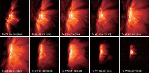
EIS observations of AR 10978 at the limb. The simultaneous observation of emission lines formed over a wide range of ionization stages provides detailed information on the temperatures and density in the million-degree corona. Observations began on 2007 December 18 at 00:10 UT. The FOV was approximately 310″ × 384″ and the exposure time at each position was 40 s. (Color online)
Figure 35 shows the results from analyzing a single loop segment in an active region presented by Warren et al. (2008). The loop was identified in Fe xii 195.119 Å and intensities for 12 emission lines were derived by fitting a Gaussian profile to the observed loop cross-section. To improve the signal-to-noise in the measurement, the profile was averaged some distance along the loop. Emission lines formed far away from 1.5 MK, such as Si vii 275.368 Å or Fe xvi 268.984 Å, showed no evidence of the loop. For these lines an intensity of zero was assumed and the uncertainty in the intensity was taken as 20% of the background in this region. The DEM was computed by assuming a Gaussian for the DEM and determining the best-fit emission measure magnitude, peak temperature, temperature width, and electron density. This analysis was applied to 20 loops observed with EIS, and in almost all cases the loops were found to have relatively narrow DEMs (σT < 0.3 MK) and relatively high densities (log ne ∼ 9.3–10.0).
![EIS has measured relatively narrow temperature distributions for many 1 MK loops. The top panel shows an EIS 195.119 Å raster over an active region, which has been sharpened to help identify the loops. The bottom panel shows the DEM computed from observations of 12 emission lines in a small segment of the loop. The emission lines range in temperature from Si vii to Fe xvi. [Adapted from Warren et al. (2008) by permission of the AAS.] (Color online)](https://oup.silverchair-cdn.com/oup/backfile/Content_public/Journal/pasj/71/5/10.1093_pasj_psz084/2/m_pasj_71_5_r1_f29.jpeg?Expires=1749038438&Signature=1UK~Y-qoYDSjJr-7si0-Sfay3wrDbO9IKGw1oY6YmcA2L-9a4TLfJhtvYJU27sJN8rT4JB5oaKWGXhKR-Uu4xuLUZKgsICC73nrfUyLbB-KSFhvy7dRqC~2l094o1MoSkeNadF0XyMxmge36004H4S~7xw4t909pX0~waDy9xvPq8fifIZTZZ6bzfuPWQBccNuFWiQLQ5VescjKSXU6R~uZKNW-zcrPKrC8Lt~XdsKS8NgDSlAC3wPLdhhu1skjWvru9-XNnwHpO0sPQERejd8~DGVESNHx~0CNheCwnbDQGby0nfx-rTXzaqRSB5n7iWqLHDtHbz8rsTZrt~DXFlg__&Key-Pair-Id=APKAIE5G5CRDK6RD3PGA)
EIS has measured relatively narrow temperature distributions for many 1 MK loops. The top panel shows an EIS 195.119 Å raster over an active region, which has been sharpened to help identify the loops. The bottom panel shows the DEM computed from observations of 12 emission lines in a small segment of the loop. The emission lines range in temperature from Si vii to Fe xvi. [Adapted from Warren et al. (2008) by permission of the AAS.] (Color online)
These EIS observations confirmed that many 1 MK loops had narrow temperature distributions, consistent with the analysis of a single loop by Del Zanna and Mason (2003) and of three-filter data by Aschwanden and Nightingale (2005). However, the analysis of other loops, Schmelz et al. (2001) and Schmelz and Martens (2006), for example, suggested relatively broad temperature distributions, and for some time there was a debate regarding isothermal and multi-thermal loops. In a study that included loops observed with EIS, XRT, and SDO/AIA, Schmelz et al. (2014) found that the width of the temperature distribution was correlated with the peak temperature, which offers a potential resolution of the controversy. Aschwanden and Nightingale (2005) noted that the number of identified loops tended to decrease sharply with temperature, indicating that most observed loops have lower temperatures and narrow DEMs. Higher-temperature loops do exist, however, and these loops tend to have broader DEMs.
The density measurements from EIS provide a way to test the assumption of loop filamentation used in the modeling of the TRACE data. Comparing the density inferred from the observed intensity and loop width with that inferred from a density-sensitive line ratio, Warren et al. (2008) concluded that loops observed with EIS were not fully resolved. Brooks, Warren, and Ugarte-Urra (2012) extended this idea, modeling 1 MK loops as a collection of identical, sub-resolution strands. They found that they could reproduce the observed cross-field intensities observed in EIS and in higher-resolution AIA data with a relatively small number of more elementary loops, typically 3 to 5, each with a width on the order of 500 km.
Observations of coronal loops at optical wavelengths have also provided support for loop filamentation. As mentioned previously, coronal loops can undergo catastrophic cooling if the coronal density becomes too high relative to the local heating rate. When this occurs, a coronal condensation forms and cool material can be observed above the limb as “coronal rain” in Hα, Ca ii H, and other cool emission lines (e.g., Schrijver 2001; Antiochos et al. 2003; Antolin et al. 2015; subsection 5.5). The spatial resolution of optical instruments such as Hinode/SOT and the ground-based SST are about 0|${^{\prime\prime}_{.}}$|15–0|${^{\prime\prime}_{.}}$|20, much higher than the 1|${^{\prime\prime}_{.}}$|2 spatial resolution of AIA. The analysis of Antolin and Rouppe van der Voort (2012) showed a mean width for coronal rain of about 310 km. Furthermore, this analysis indicated that coronal rain was often coherent, with nearby strands cooling very closely in time. Thus the observations of coronal rain support the multi-stranded loop scenario that had been adopted for the modeling of 1 MK loops.
Coronal rain is almost always observed in post-flare loop arcades. Observations with the SST and the 1.6 m NST have shown widths in these loops on the order of about 100 km (Scullion et al. 2014; Jing et al. 2016), somewhat smaller than what has been observed in non-flaring active regions.
The 2012 July 11 launch of the Hi-C instrument on a sounding rocket provided the first glimpse of the corona at 150 km spatial resolution (Cirtain et al. 2013). Unfortunately, the loop measurements from the flight have provided somewhat contradictory conclusions. Peter et al. (2013) compared several features observed in Hi-C and AIA and found no evidence for sub-structure. As illustrated in figure 36, however, Brooks et al. (2013) did find some evidence for coronal loops below the spatial resolution of AIA, but only in a few features. A very recent automated study by Aschwanden and Peter (2017) suggests that the peak in the loop width distribution measured with Hi-C is about 300 km, generally consistent with Brooks et al. (2013) as well as with the widths inferred from coronal rain.
![Evidence for loop sub-structure from simultaneous observations from AIA and higher spatial resolution Hi-C active region observations. Both images are dominated by Fe xii 195.119 Å. [Adapted from Brooks et al. (2013) by permission of the AAS.] (Color online)](https://oup.silverchair-cdn.com/oup/backfile/Content_public/Journal/pasj/71/5/10.1093_pasj_psz084/2/m_pasj_71_5_r1_f30.jpeg?Expires=1749038438&Signature=kb3obouBmNTewA~N1HYOuBZit-Um035j9IHWY-xiuP2IaMpuF9FPXlPV8YjZ~AOdR2v9MWX17XrqVyYpP8XQHtZhRS4WMxGCg3UxJgHE8rZvIlX6tMdfrP5Cb0U0uKgJnI3ZcVAqpo9BP3cPQIZfIevMBxifW8TrxXQT650NrhwToeMloVGWISrOTUHyf6IYNztB0uDWGTEWzduClLXwHcjhra~EqTh3kuS~CmdqPj0~DzA3HAFfuqOXxWO5C0wWgc94oyS5LnPzcsznGBk1kvnGSdRpuGLI1Frv~qqjTyt5YHOJ0lItUzQBGQTIMH-Lms3euzLcJzshAYf82GHWVg__&Key-Pair-Id=APKAIE5G5CRDK6RD3PGA)
Evidence for loop sub-structure from simultaneous observations from AIA and higher spatial resolution Hi-C active region observations. Both images are dominated by Fe xii 195.119 Å. [Adapted from Brooks et al. (2013) by permission of the AAS.] (Color online)
One final aspect of the multi-loop modeling of 1 MK loops is the assumption of impulsive heating. Viall and Klimchuk (2011, 2012) used the six coronal channels on AIA to systematically study the evolution of plasma near 1 MK. They performed cross-correlation analysis between the different channels in an active region and found consistent patterns of cooling between the hotter and cooler channels.
The observations appear to support the idea that 1 MK loops are generally composed of sub-resolution strands a few hundred kilometers in width that have been heated impulsively and are cooling. These loops generally have large densities relative to equilibrium and narrow temperature distributions. Unfortunately, at present it is not clear that such a heating scenario matches the observations in detail. There are some successful studies for individual cases (e.g., Warren et al. 2003; Viall & Klimchuk 2011) or limited band-passes (e.g., Kobelski & McKenzie 2014; Kobelski et al. 2014a), but no studies showing that a multi-loop, impulsive heating model can reproduce the evolution of a statistically significant sample of loops observed over a very wide range of temperatures. There are several studies that found incompatibilities between the observations and the basic predictions of hydrodynamic models (e.g., Ugarte-Urra et al. 2006, 2009; Warren et al. 2010a).
Recent work by Lionello et al. (2016) suggested that there may be a fundamental incompatibility between impulsive heating and the time delays indicated by the cross-correlation analysis. Lionello et al. (2016) suggested that the observed time lags are generally longer than what can be accounted for in hydrodynamic simulations with impulsive heating, and that thermal non-equilibrium should be considered as an alternative. Klimchuk, Karpen, and Antiochos (2010) argued that thermal non-equilibrium is not consistent with some aspects of the observations. Mikić et al. (2013) countered that loop geometry and heating asymmetries play an important role and that this heating scenario cannot be ruled out.
7.4.2 The active region core
We now turn to the high-temperature loops observed at the core of the active region that are illustrated in the right panel of figure 32. The main observational questions here are similar to those we encountered with the 1 MK loops: Are these loops bundles of sub-resolution strands that are heated impulsively? If so, we would expect the temperature distribution of the active region core to be relatively broad, since along any line of sight we should have many filaments in various stages of heating and cooling (e.g., Cargill & Klimchuk 2004).
Many of the earliest solar measurements were taken at soft X-ray wavelengths and were therefore most sensitive to high-temperature active region plasma. These measurements generally found temperatures of about 3 MK, and the authors often argued that the temperature distributions in active regions must be narrow (e.g., Evans & Pounds 1968; Withbroe 1975; Saba & Strong 1986, 1991; Schmelz et al. 1996).
Since many of these early studies used, as an indicator of temperature, broad-band soft X-ray filter or emission line ratios from observations of limited spatial resolution, these results need to be interpreted carefully. Figure 32 clearly shows that active regions are not truly isothermal. Rather, they are composed of loop structures with different apex temperatures. Furthermore, these loops undoubtedly connect to the lower layers of the solar atmosphere and thus have temperature gradients along their lengths. Thus, low spatial resolution active region observations are generally a superposition of 1 MK loops, active region moss, and core loops. As we will see, the early studies were largely correct, but this was due in part to the absence of observations over a full range of temperatures.
The EIS and XRT instruments on Hinode have provided perhaps the first opportunity to systematically study the temperature structure of high-temperature active region loops using both spectroscopy and soft X-ray imaging at relatively high spatial resolution. A typical observation of a large active region is shown in figure 37, and illustrates that we can clearly differentiate between active region core and moss emission. There is some contamination from overlying 1 MK loops in the active region core, but this contribution is relatively small.
![EIS, XRT, and AIA observations of AR 11089 on 2010 July 23 near 15:00 UT. Observations such as these have provided definitive results on the distribution of plasma in high-temperature active region loops found in the active region core. The top panels show the active region in various AIA and XRT channels. The bottom panels show EIS rasters in a few of the observed emission lines. The small box indicates the region for which the “inter-moss” DEM has been calculated (see figure 38). [Reproduced from Warren, Brooks, and Winebarger (2011a) by permission of the AAS.] (Color online)](https://oup.silverchair-cdn.com/oup/backfile/Content_public/Journal/pasj/71/5/10.1093_pasj_psz084/2/m_pasj_71_5_r1_f31.jpeg?Expires=1749038438&Signature=4Kf8DcoOdy0a1fTaFp0WR8OQbT-FuaSZsguCWX0Ah0WsbXzkj7XYYcwgLkEEvjtFxs3MSc9ekW0jzRE-Anf9O1tOrXWz8O4Wg5HOVJKNDtJZfLFQt~9xooIIP1aXFjfzt3Sn-1Repdd4SmrL7nvSx9NBk4uOC5pVOGBt05G2dW-K9VPWzEjj-JpCTKzoG-3Kk-HPLvUwV3TrToC5yn-8SgmYdxjmeKDbXvO6GmwnBkOFkdEb0PbG~FhaDz6glKuVuL1Ijrk6gou7Ty4vGtwWBtcuANOJ1TMjU7pETbOO991aTz6L7IuOIzJZPqddsqSngF8jeqNmMJrfI0MFkPsnGA__&Key-Pair-Id=APKAIE5G5CRDK6RD3PGA)
EIS, XRT, and AIA observations of AR 11089 on 2010 July 23 near 15:00 UT. Observations such as these have provided definitive results on the distribution of plasma in high-temperature active region loops found in the active region core. The top panels show the active region in various AIA and XRT channels. The bottom panels show EIS rasters in a few of the observed emission lines. The small box indicates the region for which the “inter-moss” DEM has been calculated (see figure 38). [Reproduced from Warren, Brooks, and Winebarger (2011a) by permission of the AAS.] (Color online)
Of particular significance for Hinode DEM studies are the lines from Ca xiv–Ca xvii observed with EIS. These lines have a peak temperature of formation between log Te = 6.55 and 6.75, and have relatively narrow contribution functions, at least relative to Fe xvii, which dominates broad-band soft X-ray measurements. This provides excellent temperature resolution near the peak in the active region DEM. XRT measurements complement this with a sensitivity that extends to even higher temperatures.
A DEM computed from EIS and XRT observations of a small “inter-moss” region in the core of the active region is shown in figure 38 (Warren et al. 2011a). This DEM is peaked at about 4 MK and the DEM declines sharply at both higher and lower temperatures. A survey of inter-moss areas from 15 active regions observed with EIS and AIA produced similar results (Warren et al. 2012). Further, this survey showed how the DEM varied with total unsigned magnetic flux. For the largest magnetic fluxes the DEM was strongly peaked at about 4 MK. For regions with weaker fields the peak in the DEM shifts to lower temperature and the DEM becomes broader, consistent with the results of Tripathi, Klimchuk, and Mason (2011).
![Active region core DEM computed using observations from EIS and XRT. [Reproduced from Warren, Brooks, and Winebarger (2011a) by permission of the AAS.] (Color online)](https://oup.silverchair-cdn.com/oup/backfile/Content_public/Journal/pasj/71/5/10.1093_pasj_psz084/2/m_pasj_71_5_r1_f32.jpeg?Expires=1749038438&Signature=r2ouR0SBxmtQAVfnsmJPEktHMTZs2lKkXbSJp5tZ0XFFk5D0xGuCWHNkd~GTOU7g-9gNbbgFh76YqMxgWuJgV5qWW2GR8vsr7m8xndqE6bOUztOirF-Y1STDxVxfgtySrPp~dlXFrv~aHvYBI0lLd-bZSA~u7rTj8nNq8bg4vDM1PJGZmx2RRzPrPfNreCm3JMjlGyf1wRt3URm44OeEj9rdl8hdSVxDzoqH49jfiKZfRtE6Cp3fs~2nK3bK9Cf0qIrN-W6407OJw4wMcOVD6zeoNUrAkP0Wwaq3uf~wlmmUhrhq--mi9yd4H3hCmtMwDQjFPw8ualQVRWQoGItTWg__&Key-Pair-Id=APKAIE5G5CRDK6RD3PGA)
Active region core DEM computed using observations from EIS and XRT. [Reproduced from Warren, Brooks, and Winebarger (2011a) by permission of the AAS.] (Color online)
Extensive analysis of active region temperature structure has also been carried out by Del Zanna (2013b) and Del Zanna et al. (2015). These studies found relatively steep DEMs peaked at about 3 MK throughout the active region core. The steep slopes were found to persist even on the second rotation of the active region. Furthermore, Del Zanna and Mason (2014) reanalyzed some of the Solar Maximum Mission (SMM) soft X-ray observations of non-flaring active regions using modern atomic data and DEM techniques. This work also found steep slopes at high temperatures.
One interpretation of the relatively narrow temperature distributions in the active region core is that the loops are heated steadily or are at least close to equilibrium. Movies of active regions observed with XRT, such as the movie for the data shown in figure 39, often show relatively steady emission punctuated by transient brightenings. This is consistent with the analysis of earlier SXT active region observations (e.g., Kano & Tsuneta 1995; Antiochos et al. 2003).
![Time variability of an active region observed with XRT. The left-hand panel shows a snapshot from an XRT observation of AR 11089. The right-hand panels show the light curves for three representative locations within the active region core. [Reproduced from Warren, Brooks, and Winebarger (2011a) by permission of the AAS.] (Color online)](https://oup.silverchair-cdn.com/oup/backfile/Content_public/Journal/pasj/71/5/10.1093_pasj_psz084/2/m_pasj_71_5_r1_f33.jpeg?Expires=1749038438&Signature=pKtIyQiwbNul0moI55sKnWtAzkVdm1ygdOrpQx9Uf~dUj-qPWQBxrkleH0hgEdpdinFeaEUDIFqNJ8OYMmH6izo0W1i-oMZzVQQYejbx7EUMzK~T4IRp9QPC~7blfgvZDmbsDTlzWMLRHxnqpfoxBoD49ftggMzVOCgzaOfR~APMRudYgFiagewtraIH8BoxX8AKy0UA-RZoXZc947F1O2gx~mDFM6wr2EgCDgHsLJUaVNc4QKA8raI6P4BcvBnEgQFhm-X0s0X1ppbI3hKkQmzd1H1A8Z8vEbFbjp5~Fz1vx09k8sSNlRRcpLLy2P-CazlMeLJXjtS3Nfh537HXrw__&Key-Pair-Id=APKAIE5G5CRDK6RD3PGA)
Time variability of an active region observed with XRT. The left-hand panel shows a snapshot from an XRT observation of AR 11089. The right-hand panels show the light curves for three representative locations within the active region core. [Reproduced from Warren, Brooks, and Winebarger (2011a) by permission of the AAS.] (Color online)
Of course, this behavior of the active region light curves could mask much more frequent impulsive heating events that average out to appear relatively steady (Cargill & Klimchuk 2004). Furthermore, an analysis of active region transient brightenings by Shimizu (1995) indicated that the easily observed events are not consistent with the heating requirements of an active region and are likely to be a separate population. The analysis of observations at very high cadence with XRT (Terzo et al. 2011) and with AIA Fe xviii (Ugarte-Urra & Warren 2014) indicated the presence of a population of relatively frequent events, approximately several per hour.
Cargill (2014) found that a power-law distribution of heating event magnitudes and a waiting time between events that is proportional to energy can reproduce the general properties of the observed temperature distributions. This model predicts that the frequency of heating events is comparable to a cooling time. This has important implications for models of magnetic reconnection, since it implies that the field does not fully relax to a potential state and nanoflare energies are smaller than previously imagined. Initial full-scale modeling efforts indicate that the Cargill (2014) prescription is consistent with both the observed temperature structure and temperature evolution of specific active regions (Cargill et al. 2015; Bradshaw & Viall 2016), but much more detailed modeling is required to confirm this.
Studies of non-thermal line widths suggest that the wave amplitudes in the active region core may be too small to provide significant heating there. Asgari-Targhi et al. (2015) indicated that velocities of about 30 km s−1 are needed, but studies with high-temperature EIS lines yielded non-thermal velocities of 13–18 km s−1 (Imada et al. 2009; Brooks & Warren 2016). This is generally consistent with the ground-based measurements of Ca xv by Hara and Ichimoto (1999), but much smaller than measurements reported for high-temperature emission lines observed with SMM (e.g., Saba & Strong 1991). Waves of sufficient amplitude were reported in some cases (e.g., Asgari-Targhi et al. 2014).
7.4.3 Summary of active region structures
The wealth of observations from instruments such as TRACE, EIS, XRT, and SDO/AIA have led to a significant advance in our understanding of solar active region plasmas over the past two decades. The observations clearly support the idea of time-dependent heating on unresolved loops for both the 1 MK and active region core loops. The exact nature of the heating, however, is still uncertain, and more detailed comparisons between observations and models need to be carried out.
So where do we go from here? There are several directions that look promising.
We need to look for the signatures of individual heating events (e.g., De Pontieu et al. 2009, 2011). Perhaps the most exciting work in this direction was the study by Testa et al. (2013, 2014), who showed that instruments such as HiC and IRIS appear to have the cadence and spatial resolution necessary to isolate and follow the evolution of very small-scale heating events in the solar upper atmosphere.
We need to improve our ability to extrapolate photospheric magnetic field measurements into the corona. It has long been recognized that the heating of the solar atmosphere is intimately related to the magnetic field, but we still cannot adequately describe how the field interacts with the complex environment of the solar chromosphere and forms the observed topology of the corona (e.g., De Rosa et al. 2009).
We need to routinely resolve and follow what are currently unresolved loops using both imaging and spectroscopy over the full range of temperatures. The direct observations of loops with Hi-C, observations of coronal rain with optical instruments, and the indirect evidence from modeling indicate that a spatial resolution of about 150 km with a cadence of a few seconds, and simultaneous coverage of the photosphere, chromosphere, transition region, and corona, should be sufficient to resolve these loops.
8 Flares and coronal mass ejections
8.1 Flare energy build-up: Theory and observations
8.1.1 Introduction
It is generally accepted that solar flares, prominence eruptions, and CMEs are different manifestations of a single physical process thought to be powered by the release of magnetic free energy stored in the corona prior to the activities. Storage of magnetic free energy requires non-potential magnetic fields, and it is therefore associated with shear or twist in the coronal fields away from the potential, current-free state (Priest & Forbes 2002). There are two groups of competing models for the pre-eruption magnetic configuration. One group assumes that a twisted flux rope is present in the region above the polarity inversion line (PIL) on the photosphere (Forbes & Isenberg 1991; Wu et al. 1997; Gibson & Low 1998; Krall et al. 2000; Roussev et al. 2003). The other group begins with an untwisted, but highly sheared, magnetic field (Mikic & Linker 1994; Antiochos et al. 1999a; Amari et al. 2003; Manchester 2003). In both cases, the flux rope or the sheared arcade is held down by the tension of the overlying coronal arcade.
The free energy can build up as a result of the emergence of sheared magnetic fields from below the photosphere (Leka et al. 1996; Schrijver et al. 2005; Schrijver 2007), shearing motions or rotations of the photospheric footpoints (Gesztelyi 1984; Zirin & Wang 1990), and the cancelation of flux in the photosphere (Martin et al. 1985; Livi et al. 1989). How can we explain the long-duration energy storage phase, lasting from a few days to a few weeks? Is the flux rope pre-existing or produced during eruption? Is the magnetic free energy already contained in the pre-emergence flux, and are there any contributions from the differential rotation or convective flows? Is the rotation of a sunspot driven by the Lorentz force of the sunspot’s magnetic field itself? To address these key questions we need to study the evolution of the highly non-potential region prior to, during, and after the flares. During the past decade, lots of progress has been made on flare energy storage based on Hinode observations.
8.1.2 Hinode observations
Shortly after launch, Hinode took excellent observations of one large active region, NOAA 10930, which produced a series of X-class flares. Observations made by XRT and SOT aboard Hinode suggested that the gradual formation of the non-potential magnetic fields in this active region was caused by the rotation and west-to-east motion of an emerging sunspot (Su et al. 2007; see figures 40 and 41). Min and Chae (2009) found that the positive-polarity sunspot rotated counterclockwise about its center by 540° from 2006 December 10 to 14, and the increase in the rotation speed was closely related to the growth of the sunspot. The analysis suggested that the rotation of the sunspot may have been closely related to the dynamic development of an emerging twisted flux tube. Ravindra, Yoshimura, and Dasso (2011) found that the positive-polarity sunspot rotated about 260° in the last three days, while the negative-polarity sunspot did not complete rotation of more than 20° in five days starting from 2006 December 9. The negative-polarity sunspot changed its direction of rotation five times over five days and injected both positive and negative types of spin helicity flux into the corona. The observed reversal in the sign of spinning and braiding helicity flux may have been the signature of the emergence of a twisted flux tube possessing the writhe of opposite signs, which is consistent with the findings of Tiwari (2009). Zhang, Kitai, and Takizawa (2012a) found that the main contribution to helicity accumulation came from the flux emergence effect, while the dynamic transient evolution came from the shuffling motion effect. The observational results further indicated that for AR 10930 the apparent rotational motion in the following sunspot was the real shuffling motion on the solar surface. Harra et al. (2009) found an increase in the coronal spectral line widths observed by EIS, beginning after the time of saturation of the injected helicity as measured by Magara and Tsuneta (2008). In addition, this increase in line widths (indicating non-thermal motions) started before any eruptive activity occurred. The formation and evolution of a magnetic channel structure has been reported by Kubo et al. (2007) and Wang et al. (2008). It was suggested as being formed during the emergence of a sequence of magnetic bipoles that were squeezed in the compact penumbra, and it might have been a precursor of major flares (Wang et al. 2008).
![Formation of the sheared magnetic fields observed by XRT aboard Hinode. (a)–(f) Series of X-ray images observed with the Be-thin filter by XRT from 2006 December 10 to 12. The maximum intensity (Dmax) of the XRT image is shown in the lower left corner of each panel. The SOHO/MDI photospheric magnetic inversion line is represented as a thick white line. [Reproduced from Su et al. (2007).]](https://oup.silverchair-cdn.com/oup/backfile/Content_public/Journal/pasj/71/5/10.1093_pasj_psz084/2/m_pasj_71_5_r1_f35.jpeg?Expires=1749038438&Signature=WRhIKHFjvH682mpKfqatQ7hqDZTZ2VAw5~ZP2WSGWtYMLR5X5i9WzM3cySXhc~Jnq9K7H1L3rl-NOB~npDdjmc~W-TyW4RmYTICzDyP0KqR8XuUABhTa2q3fzWMUtbMcxP-7lc~gn6E~W19C~l3MJfVO6QTayy-LI9jTKOj-SGfD~3rZJ3rIVHcSPtr5NhvX8MLu6IIQ4xllofKS4nVocGbpH6aXysIdZfqpGbsclg~gcDQPzF4yrZjR3AEBLTfFsHE-l0N-3x9F5ZbdRZaAq9g8~Vedy3-Gc9ShYXntGx0~ZniIHwb6Eqrr5sq2O2hmuQKNvnpFlGOrrW2myN2thg__&Key-Pair-Id=APKAIE5G5CRDK6RD3PGA)
Formation of the sheared magnetic fields observed by XRT aboard Hinode. (a)–(f) Series of X-ray images observed with the Be-thin filter by XRT from 2006 December 10 to 12. The maximum intensity (Dmax) of the XRT image is shown in the lower left corner of each panel. The SOHO/MDI photospheric magnetic inversion line is represented as a thick white line. [Reproduced from Su et al. (2007).]
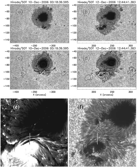
Hinode/SOT G-band images overlaid with SOHO/MDI magnetic contours. (a) and (b): G-band images closest in time to the X-ray images in figures 40a and 40f, respectively. (c) and (d): The same G-band images as in panels (a) and (b) overlaid with MDI magnetic contours. The white and black contours represent the positive and negative line-of-sight photospheric magnetic fields observed by MDI, and the thick black lines represent the magnetic inversion line. Panels (e) and (f) refer to the magnified LOS magnetogram obtained by SP and the corresponding G-band image at the peak development of the channel at around 12:00 UT on 2006 December 13. Panels (a)–(d) are taken from Su et al. (2007), and panels (e)–(f) are reproduced from Wang et al. (2008) by permission of the AAS.
Okamoto et al. (2008, 2009) studied AR 10953 and interpreted photospheric observations of changing widths of the polarities and reversal of the horizontal magn-etic field component as signatures of the emergence of a twisted flux tube. These studies supported the view that helical flux ropes emerge bodily into the photosphere rather than forming in the atmosphere once the flux has emerged. Lites et al. (2010) suggested that the formation of the filament channel in AR 10978 may be due to the emergence of a flux rope based on SOT and XRT observations. SOT observations of a rising column in a quiescent prominence were interpreted by Okamoto, Tsuneta, and Berger (2010) in terms of the emergence of a helical rope. MacTaggart and Hood (2010) constructed a dynamical flux emergence model of a twisted cylinder emerging into an overlying arcade. The photospheric signatures observed by Okamoto et al. (2008, 2009) were seen in the model, although their underlying physical mechanisms differ. Green and Kliem (2014) presented the evolution of four active regions, shown in figure 42. The evolution of the coronal configuration was driven by the motions of the photospheric plasma, and was seen in this study to pass through three stages as the arcade field evolved into a flux rope (Green et al. 2011). During the first stage, shear in the coronal arcade field increased due to photospheric motions associated with flux emergence or flux dispersal and flux cancelation, and filaments started to form. During stage two there was an accumulation of a significant amount of axial flux running along the PIL as flux cancelation, further shearing, and/or rotation of the magnetic polarities took place. The remnant arcade field showed the appearance of two J’s on either side of this axial flux. In stage three, flux cancelation produced field lines that were twisted around the axial flux and supplied poloidal flux to the rope.
![Evolution of sigmoidal active regions observed by XRT showing the three phases of evolution from flux emergence to sheared arcade, to “double J”-shaped loops, and then finally the continuous S-shaped threads of the sigmoid. Top row: AR 10930. Second row: AR 8005. Third row: Unnumbered region observed on the disk during 2007 February. Bottom row: AR 10977. [Reproduced from Green and Kliem (2014).] (Color online)](https://oup.silverchair-cdn.com/oup/backfile/Content_public/Journal/pasj/71/5/10.1093_pasj_psz084/2/m_pasj_71_5_r1_f37.jpeg?Expires=1749038438&Signature=LahXWU2a43u-6Wo3v1Ree7QYfUfqKu5ibRE0sss07kNod8U-LefndWFZnbTpWqVOUmtIsKv9Ic12j~74tqtHQ46eTJOPX3PoMhk-FpFiRHoAa9G76XWFbzPkASyHEqNq75sdpFjkPlPNWvA5G5uhzvkP6Enp4wgVu-Mj1ICWTes06aVnha95Ch9jZBe27t9zdQ45tnRdjF-hQgcRf38C1DAMaaqJ5f~C8j3OuT4x5ei-YtZwEkX6QXOjdWSMh7CLbKyb9L4uQ6M1zDkHWlwsGqj8xlfllN2x9FjSvUdkfktLhyP78clWBn0H-r8A52C2A-Hidbk-FZNVRmVbML81xw__&Key-Pair-Id=APKAIE5G5CRDK6RD3PGA)
Evolution of sigmoidal active regions observed by XRT showing the three phases of evolution from flux emergence to sheared arcade, to “double J”-shaped loops, and then finally the continuous S-shaped threads of the sigmoid. Top row: AR 10930. Second row: AR 8005. Third row: Unnumbered region observed on the disk during 2007 February. Bottom row: AR 10977. [Reproduced from Green and Kliem (2014).] (Color online)
Shimizu, Lites, and Bamba (2014) observed high-speed flows along the flaring PIL which lasted for several hours before and after the X5.4 flare on 2012 March 7 (SOL2012-03-07T00:24).13 This study suggested that the observed shear flow increased the magnetic shear and free energy that powered this major flare.
8.1.3 Simulation and theory
Theoretical studies of the flare energy build-up process are divided into two parts: magnetic field modeling of the static coronal configuration and MHD simulation of the dynamic evolution. We first review the 3D extrapolation of the coronal magnetic fields from measurements of the photospheric field.
The 3D coronal magnetic field cannot be observed routinely, although progress has been made (Judge 1998; Solanki et al. 2003; Lin et al. 2004). The non-linear force-free field (NLFFF) is considered to be the most realistic way of reconstructing the coronal field. Various methods of obtaining NLFFF solutions to model the active region’s magnetic fields have been proposed and developed in the past decade (for details please refer to Schrijver et al. 2006; Metcalf et al. 2008; Wiegelmann & Sakurai 2012; Wiegelmann et al. 2014, 2017; Inoue 2016; Guo et al. 2017). Many difficulties arise when solving the problem of constructing an NLFFF based on the observed photospheric vector magnetograms. Different methods for solving the NLFFF problem, and even different implementations of the same method, applied to the same photospheric data, and even the same method applied to different polarities of the same data, have frequently yielded results inconsistent with each other and with the coronal features (Schrijver et al. 2006, 2008; Metcalf et al. 2008; De Rosa et al. 2009). Although the NLFFF remains problematic, several recent studies have roughly captured the observed non-potential structures, as well as the storage-and-release processes of magnetic energy and helicity.
Various magnetic field reconstruction algorithms have been adopted to study the flare-productive AR 10930 based on Hinode/SOT photospheric magnetic field observations. NLFFF extrapolations showed that the general topology of this active region could be described as a highly sheared core field and a quasi-potential envelope arch field (Guo et al. 2008; Schrijver et al. 2008; He et al. 2011), and the modeling was suggestive of an emerging twisted flux rope. Using a linear force-free field model, Magara (2009) found that the magnetic shear first increased in magnitude and area with time, while it decreased before the onset of the flare. A relation between the evolution of magnetic shear and the motions of an accompanying sunspot has also been found. These results were suggested to be caused by the emergence of a twisted flux tube into the atmosphere. Inoue et al. (2012b) revealed that the magnetic flux was twisted more than a half turn and gradually increased during the last day prior to the onset of the flare, and that it quickly decreased for 2 hr after the flare. This is consistent with the storage-and-release scenario of magnetic helicity. Using axisymmetric linear and NLFFFs in a spherical shell geometry, Prasad, Mangalam, and Ravindra (2014) found that the free energy and relative helicity of the active region peaked before the flare. Park et al. (2010) found that the time profile of the coronal helicity showed a good correlation with that of the helicity accumulation by injection through the surface. This flare was preceded not only by a large increase of negative helicity in the corona over 1.5 d, but also by noticeable injections of positive helicity through the photospheric surface. They conjectured that the occurrence of the X3.4 flare was related to the positive helicity injection into an existing system of negative helicity. For AR 11884, Yan et al. (2015) showed that a shearing motion of the opposite magnetic polarities and the rotation of the small sunspots with negative polarity played an important role in the formation of two active region filaments. Twisted structures were found in the two active region filaments prior to their eruptions from NLFFF extrapolations. NLFFF reconstructions for AR 10953 by Canou and Amari (2010) also exhibited a twisted flux rope in the pre-flare configuration. Malanushenko, Longcope, and McKenzie (2009) developed a method that built a simple uniformly twisted magnetic field and adjusted its properties until there was one line in this field that matched one coronal loop (e.g., observed by XRT). Using this method, Malanushenko, Yusuf, and Longcope (2011) demonstrated that the rate of change of twist in the solar corona was indeed approximately equal to that derived from the photospheric helicity flux.
The flux rope insertion method developed by van Ballegooijen (2004) uses a forward modeling approach to build a set of different NLFFF models and then select the model that best fits the coronal (XRT) and chromospheric (e.g., SOT) observations. This method has been adopted to study the evolution of three active regions prior to the flare, and the models were constrained by the observed X-ray and EUV loops (Savcheva & van Ballegooijen 2009; Su et al. 2009b, 2009c; Savcheva et al. 2012a, 2012b, 2012c). The modeling showed that a highly sheared and weakly twisted flux rope embedded in a potential field described very well the X-ray non-potential active region core structure. Su et al. (2009c) found that two J-shaped sets of loops were merged into a longer one, and brighter non-potential loops appeared during the day before the eruption. Su et al. (2009c), Savcheva and van Ballegooijen (2009), and Savcheva et al. (2012b) found that free energy gradually built up before the eruption, which was due to flux cancelation observed in the photosphere. A successful eruption will occur when the axial flux in the flux rope is close to the threshold of instability, and vice versa.
In the force-free approximation the NLFFF is reconstructed for equilibrium states, so that the onset and dynamics of solar flares and CMEs cannot be obtained from these calculations. For the 2007 December sigmoid, Gibb et al. (2014) performed a simulation using magnetofrictional techniques driven by observed LOS magnetograms (Mackay et al. 2011). They found the formation of a flux rope across the PIL at the same location as the observed X-ray sigmoid during flux cancelation. Fan (2011, 2016) carried out 3D MHD simulations to model the initiation of the CME of 2006 December 13. The author found that the emergence of an east–west-oriented twisted flux rope whose positive (following) emerging pole corresponded to the observed positive rotating sunspot emerging against the southern edge of the dominant pre-existing negative sunspot. With continued driving of flux emergence, the reformation of a coronal flux rope set the stage for the second eruption. This may explain the build-up of the following X-class eruptive flare the next day.
To determine the flare dynamics in a realistic situation, MHD simulations using the NLFFF as an initial condition have been proposed (Jiang et al. 2013; Kliem et al. 2013; Amari et al. 2014; Inoue et al. 2014). The simulation results have begun to reveal complex dynamics, some of which have not been inferred from previous simulations of hypothetical situations, and they have also successfully reproduced some observed phenomena; for details please refer to the reviews by Inoue (2016), Guo, Cheng, and Ding (2017), and Wiegelmann, Petrie, and Riley (2017). For example, NLFFF extrapolations by Amari, Canou, and Aly (2014) within four days prior to the X-class flare of 2006 December 13 in AR 10930 (SOL2006-12-13T02:40) showed that the magnetic free energy increased with time, and a twisted flux rope formed several hours before the eruption. This solution was then used as the initial condition, and the model was evolved dynamically by adopting photospheric changes (such as flux cancelation). When the magnetic energy stored in the configuration was too high, no equilibrium was found and the flux rope was “squeezed” upwards. The subsequent reconnection drove a mass ejection.
From the theoretical point of view, two mechanisms can account for the flare energy storage (Janvier et al. 2015): One is the emergence of sub-photospheric current-carrying flux tubes from the convection zone. Leake, Linton, and Török (2013) presented results from 3D visco-resistive MHD simulations of the emergence of a convection zone magnetic flux tube into a solar atmosphere containing a pre-existing dipole coronal field. They observed that the emergence process is capable of producing a coronal flux rope by the transfer of twist from the convection zone. The process of emergence and equilibration of twist supported the conclusions from observations that sunspot rotation is driven by twisted flux tube emergence and that it can cause the formation of sigmoids prior to a solar flare. MHD simulations by Archontis et al. (2009) showed that flux emergence of a twisted flux tube below the photosphere leads to the formation of the two J-shaped structures, then an additional current layer forms the overall S-shape due to reconnection. The central brightening is accompanied by the eruption of a flux rope from the central area of the X-ray sigmoid. Another mechanism that can account for the formation of a current-carrying magnetic field is slow photospheric motions, for example by twisting the polarities, or by inducing shearing motions parallel to the inversion line. Moreover, flux ropes can form by reconnection of low field lines, such as in the model of van Ballegooijen and Martens (1989). The simulation of Aulanier et al. (2010) forms a flux rope structure via photospheric motions (twisting) and diffusion at the photosphere. Simulations from both mechanisms can reproduce well the shape of the 2007 February 12 sigmoid—see figure 5 in Janvier, Aulanier, and Démoulin (2015).
Prior to the Hinode era, Magara and Longcope (2003) carried out 3D MHD simulations to study magnetic energy and helicity injection into the atmosphere as a result of flux emergence. This process is basically carried out by shearing motions and emerging motions at the base of the atmosphere. During the early phase of emergence, the emerging motions play a dominant role in injecting energy and helicity while the photospheric area of magnetic regions is expanding. As the emergence becomes saturated, however, the magnetic field distribution deforms and fragments by shearing motions, and these motions become the main contributor of energy and helicity injection into the atmosphere. Recently, Fang et al. (2012a, 2012b) performed MHD simulations to address the emergence of magnetic flux ropes from a turbulent convection zone into the corona and found both shearing and rotational flows driven by the Lorentz force. These horizontal flows were found to dominate the energy transport from the convection zone into the corona. Shear flows, converging motions, and tether-cutting reconnection combined to continuously build up the magnetic shear and free energy in the corona necessary for eruptive and explosive events. It was the long-lasting, Lorentz-force-driven shearing motion that dominated the energy transfer. For a detailed review of flux emergence please refer to Fan (2009), Cheung and Isobe (2014), Schmieder, Archontis, and Pariat (2014), Janvier, Aulanier, and Démoulin (2015), van Driel-Gesztelyi and Green (2015), and Inoue (2016).
8.1.4 Summary
Hinode’s observational characteristics of flare energy build-up processes include flux emergence, shearing motion, sunspot rotation, helicity injection, flux cancelation, and shearing and converging flows. In particular, sigmoid structure may be formed via emergence of twisted flux ropes and/or flux cancelation, which is associated with the increase of free energy and helicity. An increasing number of observational studies and NLFFF simulations have suggested that a flux rope can be formed hours before the onset of the eruption. The mechanism of flux rope formation via magnetic reconnection driven by flux cancelation fits very well for decaying active regions. For an emerging active region, some studies suggested that it is formed via bodily emergence from the convection zone, while others suggested that it is formed through reconnection driven by photospheric motions. This is still under debate, and should be the subject of further study.
Rotational motions of and around sunspots have been observed by many authors over many decades [see Brown et al. (2003) and references therein], and have suggested that the rotational motion of a sunspot may be related to the energy build-up and later release by a flare. The proposed mechanisms regarding the origin of the observed sunspot rotation include Coriolis force and differential rotation, photospheric flows, expansion of the coronal segment of a twisted flux rope, and so on [see Brown et al. (2003), Min & Chae (2009), and references therein]. Sunspot rotations were found to be driven by the Lorentz force in earlier simulations (Fan 2009; Longcope & Welsch 2000), and the simulation by Fang et al. (2012a) illustrated that this rotation mechanism operates in a realistic convection zone. A case study of Hinode observations by Zhang, Kitai, and Takizawa (2012a) suggested that the apparent rotational motion in the following sunspot is the real shuffling motions on the solar surface. Further analysis is still required to determine the primary mechanism for the cause of the observed rotating sunspots.
It is worth noting that most of the present studies are focused on the energy build-up in active regions. How is the energy built up in quiescent prominence eruptions? Is it the same as that of active region flares? This is still an open question. Other open questions include, but are not limited to, the role of resistive flux emergence (Pariat et al. 2004; Isobe et al. 2007b) in the structure formation and energy build-up in an AR.
8.2 Flare observations: Energy release and emission from flares
Prior to the launch of Hinode, the broad elements of those aspects of a flare model concerned with the release of energy and emission from solar flares had already taken shape. The release of stored coronal magnetic energy, facilitated by magnetic reconnection, results in the acceleration of non-thermal particles, the energy and spatial distribution of which can be constrained from hard X-rays which appear both in the corona and the chromosphere (Krucker et al. 2008; Fletcher et al. 2011), as measured by instruments such as the Yohkoh Hard X-ray Telescope (HXT; Kosugi et al. 1991) and RHESSI spacecraft (Lin et al. 2002). As the flare proceeds, ribbons of emission, most readily identified in Hα and UV (Asai et al. 2004; Qiu 2009) spread across the chromosphere, identifying the heated chromospheric footpoints of the just-reconnected field, as the coronal reconnection develops. Some parts of the ribbon also emit in the optical (Matthews et al. 2003; Hudson et al. 2006), usually co-spatial with hard X-ray sources, identifying these as the most intense source of energy dissipation. One result of flare heating of the chromosphere is expansion—the so-called “chromospheric evaporation”—which can be very rapid (explosive) at speeds approaching the speed of sound if the energy deposition rate is very high, and accompanied by momentum-balancing downflows at lower temperature. Evaporation leads to the filling and brightening of soft X-ray coronal loops, which cool and drain over time scales as long as hours.
Flares, whether eruptive or not, tend to fit this general scenario very well. However, many questions remain, both fundamental and more peripheral. Most fundamental is how the energy, previously stored (we think) in large-scale coronal current systems, is converted on time scales of seconds into the non-thermal and thermal kinetic energy of the plasma particles, and observations from EIS point us towards a fundamental role for turbulence (Jeffrey et al. 2017; Kontar et al. 2017). Linked to this is the question of how the magnetic field changes during reconnection, and when energy is removed from it, and here SOT, EIS, and XRT show us different aspects of the magnetic “convulsion” that is central to the flare. Flare energy conversion is also bound up with another basic problem, that of energy transport from the corona, where the energy is stored, to the chromosphere, where most of it is dissipated. The prevailing model postulates that energy transport is by beams of non-thermal particles accelerated in the corona (most models say near the coronal reconnection site) which stream down the field to the chromosphere where they are collisionally stopped, resulting in heating. However, the beam model is being challenged, in part by SOT observations, which when combined with RHESSI put strong constraints on the beam electron flux. SOT observations have also allowed us to progress on perhaps the oldest problem in solar flare physics—what causes the flare white-light emission, which embodies the majority fraction of a flare’s radiative flux? The heating and flows of the chromosphere in response to intense flare energy input, and the cooling and relaxation of the corona, are on the face of it less complex than the energy conversion and transport problems; however, there are still unsolved problems. For example, the cooling of the hottest loop plasma, at XRT temperatures, takes longer than expected from conduction or radiation alone, and may point to ongoing slow energy input.
Solar flares emit across the entire electromagnetic spectrum, so the Hinode mission with its three instruments sampling between the optical and the soft X-ray wavelengths, with a combination of broad- and narrow-band imaging and spectroscopy, is ideally placed to pursue many of these basic questions related to flares.
To facilitate flare research, particularly multi-instrument research, the Hinode mission has produced a flare catalog (Watanabe et al. 2012) which can be found online.14
8.2.1 Optical measurements
As is well known, the first observations of a solar flare were made in the optical (Carrington 1859), which is where the majority of a solar flare’s energy is released. It is, however, difficult to detect flares in the optical because of their relatively low contrast against the photospheric background and their transience. We know from previous work with the TRACE satellite (Hudson et al. 2006) that a cadence of 2–4 s is able to capture the optical flashes from small flares, and Hinode/SOT tended to have a lower cadence than this. However, several excellent optical flare observations have been made, and in these the notable advantages compared to what was achievable with the TRACE satellite are the spatial resolution, of around 0|${^{\prime\prime}_{.}}$|2, and the occasional three-color imaging through SOT’s BFI red, green, and blue (RGB) broad-band filters. This allowed some constraints to be put on the underlying optical continuum spectrum, and hence the emission mechanism. G-band flare observations were more common than RGB, but these are not true continuum, and the flare ribbon area measured in the G-band may overestimate the optical flare area as measured in the blue continuum; Wang (2009) found a factor of 10 difference in area in one case, though this may just be a contrast effect. A survey of two years of SOT flares in the Hinode early mission by Wang (2009) found seven G-band flare observations out of 13 candidates observed by SOT, and concluded that in its usual mode of operation SOT is likely to be able to detect flares in the G-band above GOES M1.0 class. Peak G-band contrasts can be up to a factor 2–3.
The measured area of flare ribbons observed by SOT has been used to construct arguments about the flare energy transport. In the standard model for flare energy transport a beam of mildly relativistic (a few tens of keV) electrons carry the flare energy from the corona to the chromosphere where they stop collisionally, giving up their energy and heating the chromosphere and, possibly, also the photosphere. In establishing the viability of this model, one of the critical parameters is the inferred beam density. In a study of the flare of 2006 December 6 (SOL2006-12-06T18:47) using both SOT G-band observations and RHESSI hard X-ray (HXR) images at a nominal resolution of 1|${^{\prime\prime}_{.}}$|8 (figure 43), Krucker et al. (2011) found that a very high coronal electron beam density was required to explain the observations—on the order of 1020 electrons cm−2 s−1, which would constitute a significant fraction of all electrons in a coronal loop rooted in the HXR source. This poses a challenge for the electron beam model. The G-band observations in this case were used to help constrain both the total luminosity of the flare footpoint, and its area. In the flare of 2006 December 14 (SOL2006-12-14T22:15) Watanabe et al. (2010a) found that the energy for the G-band enhancement—assuming this was part of an enhanced (photospheric) blackbody continuum, which is a conservative assumption—could be provided by electrons above 40 keV. Such electrons will stop collisionally relatively high in the chromosphere and cannot excite a blackbody continuum directly. This possibly points towards the emission being instead a recombination continuum formed higher up in the chromosphere, or partly due to photospheric backwarming, where that continuum also heats the lower chromosphere/photosphere from above.
![G-band image of the flare of 2006 December 6 (SOL2006-12-06T18:47) with contours of RHESSI 25–100 keV emission superimposed. The excellent spatial correspondence and well-resolved RHESSI sources allowed strong constraints to be put on the electron energetics in this event. [Reproduced from Krucker et al. (2011) by permission of the AAS.] (Color online)](https://oup.silverchair-cdn.com/oup/backfile/Content_public/Journal/pasj/71/5/10.1093_pasj_psz084/2/m_pasj_71_5_r1_f38.jpeg?Expires=1749038438&Signature=q8qLT83UnG-QEBdmMQ0ohxaApRtzjnu0GiMiCkwSVnGIhpmOotNgWxB5XShYZetR~3AncXQA2ImwsG-QUlWgfYay64KhfX6INDU4fYgXBoP24MMErLMym1o75Cez0V1WLBNV0gtPb2QN5RC8S489YdV6hAPW-HU39XT9Cetc~uglgNn1k2W2Z6ASyNvLFs4VbVpY4iBZh0NiYL5aqZsmOswbMv8xCm0nnaepQPHYl09gia2U6siAMGfqP2c-jux7WXBHIr9YR57wspvO07FDrvoKtgj6276aufTm3ES-1emc~8~EUWodHmbc5HgFLKJeYGpsn~8W3khv1DuZlYXhZg__&Key-Pair-Id=APKAIE5G5CRDK6RD3PGA)
G-band image of the flare of 2006 December 6 (SOL2006-12-06T18:47) with contours of RHESSI 25–100 keV emission superimposed. The excellent spatial correspondence and well-resolved RHESSI sources allowed strong constraints to be put on the electron energetics in this event. [Reproduced from Krucker et al. (2011) by permission of the AAS.] (Color online)
The character of the flare optical spectrum is not well known, but is critical for understanding the location of energy deposition and hence the mechanism of flare energy transport. Using SOT-BFI RGB continuum data, Kerr and Fletcher (2014) set constraints on the flare spectrum and energy content for the flare of 2011 February 15 (SOL2011-02-15T01:56), fitting the three-point “spectrum” either with a blackbody function or a free-bound continuum model. In some parts of the flare ribbons, the color temperatures and the blackbody temperature were found to be the same within errors, suggesting a blackbody temperature increase of a few hundred kelvin. In other locations the data were more consistent with recombination emission from an optically-thin slab at a temperature between 5500 K and 25000 K. These data can also be used to constrain the optical luminosity over a broad range (∼2000 Å) of the optical spectrum, at either around 1026 erg cm−2 s−1 for the blackbody case or an order of magnitude more for the recombination emission case. They were used as part of an overall assessment of the chromospheric/photospheric radiation budget of a flare by Milligan et al. (2014), demonstrating that the near-UV to optical part dominates the total energy.
The high resolution of SOT of course permitted detailed study of flare spatial structure within footpoints and ribbons. In the flare of 2006 December 13 (SOL2006-12-13T02:40) Isobe et al. (2007c) found ribbons in the G-band consisting of bright leading kernels around 500 km across, followed by a trailing, more diffuse region that appeared optically thin. The structure was interpreted by the authors as due to direct heating in the kernel and backwarming of the photosphere forming the diffuse region, but the diffuse region could also be optically-thin recombination emission. The vertical structure of SOT flare footpoints in the BFI RGB filters was examined in the flare of 2012 January 27 (SOL2012-01-27T18:37), which occurred very close to the limb, by Watanabe et al. (2013), who found a displacement of 400 km between red (upper) and blue (lower) sources of emission, simultaneous within 6 s, and for a claimed accuracy in alignment of 70 km (figure 44). If this displacement indeed corresponds to a vertical offset, with the red and blue emission centroids at substantially different locations, an explanation in terms of a single-temperature blackbody seems unlikely. Arguments about the absolute location for these SOT sources are unfortunately still indirect, relying on inferences from the quiet Sun, but future radiation hydrodynamics modeling will help here (sub-subsection 8.2.4).
![Distribution of footpoint intensity in Hinode/SOT RGB filters, and Ca ii H in a limb flare, as a function of height, compensated for the longitude of the flare source. Note, the heights are relative; the absolute location of the photosphere (τ500 = 1) does not correspond to the zero point. The offset between peaks suggests that the different color optical sources are primarily formed at different altitudes. [Reproduced from Watanabe et al. (2013) by permission of the AAS.] (Color online)](https://oup.silverchair-cdn.com/oup/backfile/Content_public/Journal/pasj/71/5/10.1093_pasj_psz084/2/m_pasj_71_5_r1_f39.jpeg?Expires=1749038438&Signature=KOhUXU75Nkv2mhwfPCtBMuJoykSxdoUOvXwrwSR9Cw80yY48S6ER3ybRpegPWgY6cMDGrGMOeIUIMaiQTw7Gddd7Q~slrj9MUrAIGulz8a18Vn7VIPHO-hAeNdQcGx-lNoBx~wCDZF2oM9tTHubXY4UTONLBgEG0A7ol4mBE34LpR6kErOS-DxF~DuRE5qmZSejDiMUwIqGZG7TkGGZ9~OphJ48Tmb2WU4czgGAs9cYaNsGOGx37EFTk1~41eM7OmS~jKsZ46x4FQj0YpCAdH3B8lPHQyMFxVjTY0OKxRMOnWqyxkdYwtarYzBO9VSDRL1gA7tK9qwGP~TZUc40iHQ__&Key-Pair-Id=APKAIE5G5CRDK6RD3PGA)
Distribution of footpoint intensity in Hinode/SOT RGB filters, and Ca ii H in a limb flare, as a function of height, compensated for the longitude of the flare source. Note, the heights are relative; the absolute location of the photosphere (τ500 = 1) does not correspond to the zero point. The offset between peaks suggests that the different color optical sources are primarily formed at different altitudes. [Reproduced from Watanabe et al. (2013) by permission of the AAS.] (Color online)
Detailed SOT observations of the evolution of the photospheric magnetic field during flares have also been illuminating. For example, the fine spatial scales of SOT magnetograms compared to those from previous instruments allowed Jing, Chae, and Wang (2008a) to examine carefully the relationship between flare footpoints in the G band and the reconnection rate (ribbon speed × normal component of magnetic field), finding that G-band flare footpoints occurred at locations where both line-of-sight field and reconnection rate had high values, in common with some previous results at lower resolutions. Hinode’s photospheric vector field measurements have substantially added to our understanding of the photospheric field variations at the time of major flares, with several reports of non-reversing changes in the magnetic field strength and direction. Non-reversing field changes at the time of flares had previously been seen in line-of-sight observations (Cameron & Sammis 1999; Kosovichev & Zharkova 1999; Sudol & Harvey 2005), but the high-spatial-resolution Hinode/SOT observations were the first convincing observations of changes in the vector field. These were used by Jing et al. (2008b) to examine the variation of magnetic shear across the PIL in SOL2006-12-13T02:40. They found an increase in non-potentiality at heights less than 8000 km above the photosphere, and a decrease above 8000 km, indicating a possible altitude above which the flare energy was released. Liu et al. (2012) identified a downward “collapse” of the core magnetic field in the flare of 2011 February 13 (SOL2011-02-13T17:38) at or near the time of the flare. Changes to the photospheric field also occurred in the penumbra of sunspots where flares possibly coincided with the reorientation (Gosain et al. 2009) of penumbral fibrils, or even their disappearance (Wang et al. 2012a) as the penumbral field presumably became much more vertical during the flare. This phenomenon, among others, has been reviewed by Wang and Liu (2015).
8.2.2 Imaging spectroscopy in the EUV
The EIS instrument has produced many results on the properties of EUV-emitting plasmas. A recent review of EUV spectroscopy of the chromosphere with EIS and SDO/EVE was given by Milligan (2015). High-quality EUV imaging spectroscopy observations of the flare chromosphere were rare prior to EIS—though see SOHO/CDS observations by Czaykowska et al. (1999) and Milligan et al. (2006a, 2006b)—and EIS has made several discoveries as well as firming up much of what was suspected from previous observations.
During a flare, the lower atmosphere emits in EIS lines normally thought of as coronal lines due to their high formation temperatures (e.g., Watanabe et al. 2010b), but the emission sources are compact, reasonably dense ribbons and footpoints (figure 45) with electron densities inferred from EIS diagnostic ratios of a few × 1010 to |$10^{11}\:\rm {cm}^{-3}$| at around 1.5 MK (Del Zanna et al. 2011b; Graham et al. 2011; Young et al. 2013), and up to |$10^{12}\:\rm {cm}^{-3}$| at 2.5 × 10⁵ K (Graham et al. 2015). The interpretation is that the flare rapidly heats the upper chromosphere (as defined in terms of density) to temperatures that can be as high as 10 MK. The chromospheric emission-measure distribution obtained in a number of flares by Graham et al. (2013) was found to peak at about 10 MK, with a gradient between 105 and 107 K that is consistent with (though not necessarily explained solely by) thermal conduction. It must be recalled that standard EUV density diagnostics assume equilibrium ionization and Maxwell–Boltzmann distributions of electrons; both of these assumptions must be questioned under flare conditions. However, Bradshaw (2009) established that at densities of a few × 1010 cm−3 and at these temperatures, the plasma is sufficiently collisional for equilibrium ionization to be established. The effect of relaxing the latter assumption can now be examined for kappa distributions (Dzifčáková et al. 2015).
![Density maps of the lower atmosphere in a small flare observed with Hinode/EIS at different times. The left-hand and center rasters are separated by 8 min, and the center and right-hand images by 29 min. The brightest regions correspond to the ribbons and bright footpoints of this small flare. [Reproduced from Graham, Fletcher, and Hannah (2011) by permission of ESO.] (Color online)](https://oup.silverchair-cdn.com/oup/backfile/Content_public/Journal/pasj/71/5/10.1093_pasj_psz084/2/m_pasj_71_5_r1_f40.jpeg?Expires=1749038438&Signature=vvO0FfelT8O2eCuiW~no1sQU3omw6bovjA9wu5Xw3RkGiDAY7bNG~fJZpNUZ-oRIV8jq~fB-~ntFxwpmt-lTc9Fld01JM-OwCzhs1fQqdFeGN1rl5nZtp5Rb7AJLuy7jvHgzBdALMKl-7X5h9-cOhTEjRIZue-FvOgwoqd7gVBWyZE7zTmPyC61gzfeWyyZBy21h2q2DdTq38vmJtrLLSJIPnZB5HgS9BBsWPqkjGMTrWvC2-cG7GRXX8DMhsL65DUCe95O9cDHHlqkHyiqOJcgBPRdrl4CVWLMJG1KQuSjOV~I-wuSjaac8fXKQZFZHOA489fT2KOnfORHmqdJFsw__&Key-Pair-Id=APKAIE5G5CRDK6RD3PGA)
Density maps of the lower atmosphere in a small flare observed with Hinode/EIS at different times. The left-hand and center rasters are separated by 8 min, and the center and right-hand images by 29 min. The brightest regions correspond to the ribbons and bright footpoints of this small flare. [Reproduced from Graham, Fletcher, and Hannah (2011) by permission of ESO.] (Color online)
EIS is ideally suited to examine the multi-thermal flows originating from this heated chromospheric plasma, and this revealed a pattern of flows characterized by blueshifts of up to 250–300 km s−1 in hot lines (temperature of peak formation ≳2 MK), with the flow speed increasing with temperature (Milligan & Dennis 2009; Del Zanna et al. 2011b; Brosius 2013; Doschek et al. 2013; Young et al. 2013). Below about 1.5 MK the flows tend to be redshifted by a few tens of km s−1. This pattern has been interpreted as evaporation and condensation flows, though the downflows were at higher temperatures than previously expected. The model of Liu, Petrosian, and Mariska (2009), which combined hydrodynamic simulations of atmospheric response with stochastic particle acceleration and transport, predicted a downflow at these temperatures. The downflow is in part due to the character of the electron energy distribution at low energy (no low-energy cutoff value), which means more energy is lost in the less dense upper part of the atmosphere leading to higher temperatures and stronger flows.
There is a long-standing debate about whether there is a “stationary component” in high-temperature flare lines, i.e., whether all the plasma observed at temperatures in the 10 MK range is evaporating or whether there is also some static hot plasma. A stationary component was detected in spatially unresolved observations and explained as due to the dominance of evaporated material that had come to a halt at the top of coronal loops, but a stationary component is also dominant in individual EIS flare footpoints, in lines of Fe xxiii and Fe xxiv (Milligan & Dennis 2009), in contradiction to model expectations. This has been examined by EIS and IRIS in combination (Graham & Cauzzi 2015; Polito et al. 2016); IRIS has shown beyond doubt that at a time resolution of ∼10 s and a pixel scale of 0|${^{\prime\prime}_{.}}$|33 (around three times finer than the EIS pixel size) the emission at ∼10 MK detected in the Fe xxi 1354.1 Å line was wholly blueshifted. An apparent stationary component is likely to be at least in part the result of undersampling, in space and/or time, a very rapidly varying phenomenon, so that plasma at different speeds is unresolved within an EIS pixel. This is not yet completely established by observations: Polito (2016) carried out the exercise of binning over several IRIS pixels to mimic EIS resolutions and, though more emission was seen at the rest wavelength of Fe xxi, blueshifted emission still dominated, contrary to the EIS observations of the same event. However, agreement may be found when time evolution is also taken into account.
As well as flows, presumably along the magnetic field, associated with chromospheric evaporation and condensation, EIS has revealed flows in the flare corona. Spectroscopic detections of hot, upward outflows and cooler inflows around the expected site of flare reconnection were made during the impulsive phase of the flare of 2007 May 15 (SOL2007-05-19T13:05) by Hara et al. (2011). Simões, Graham, and Fletcher (2015) also detected strong redshifts (40–250 km s−1) in what appears to be a coronal source in the flare of 2013 November 9 (SOL2013-11-09T06:38), which was close to disk center (figure 46). This is very suggestive of rapid loop retraction following reconnection, as is the observation of Imada et al. (2013) of hot (30 MK) fast (500 km s−1) flows above an arcade on the limb during the rise phase of SOL2012-01-27T18:37.
![Top: EIS velocity measurements in a coronal loop between two flare ribbons. Bottom: Overall geometry seen in AIA (94 Å in background, 1200 Å in black contours), which implies that the EIS measurements correspond to rapid downflows (loop retractions) from a reconnecting coronal site. [Reproduced from Simões, Graham, and Fletcher (2015) by permission of ESO.] (Color online)](https://oup.silverchair-cdn.com/oup/backfile/Content_public/Journal/pasj/71/5/10.1093_pasj_psz084/2/m_pasj_71_5_r1_f41.jpeg?Expires=1749038438&Signature=RfbzX7kCciCogNrHD4tZiZBETC9CTxzwbLOj-XM39D3LyXsZyZE3DSW88rPStQnDqKZ9wv76U7Mexo2Jbee9vk6hzIrIgIdcAre-Z4gmb1FSrJgqoBjGMPA3-6qVuI-NFQiPfEvPbyhEE2huJ9rAZHpjWbdABaYef9sb-uZ1nsv9jh~CT92~APkz~OPVGYFPduIjX3YbL7CxzHX7I~fG2BbOc9vB6xxuhuKqNJRbqx-nWE4e7Rj7ihSa37YRcAfN8ygHOq5dC-zXhlO5l-OAk8SM2vX7SJY40KUyyfH4sNANDFZwvng1rjVfsfb9DtJOoauW5EZ6lE15RO9njgMozg__&Key-Pair-Id=APKAIE5G5CRDK6RD3PGA)
Top: EIS velocity measurements in a coronal loop between two flare ribbons. Bottom: Overall geometry seen in AIA (94 Å in background, 1200 Å in black contours), which implies that the EIS measurements correspond to rapid downflows (loop retractions) from a reconnecting coronal site. [Reproduced from Simões, Graham, and Fletcher (2015) by permission of ESO.] (Color online)
Spectral lines which are broadened in excess of their expected thermal widths (convolved with the instrumental width) have been convincingly observed in flares with EIS, in the flare corona (Hara et al. 2008b; Doschek et al. 2014) as well as recently around pre-eruption flux ropes (Harra et al. 2013). Fe xxiv line broadening at the top of a flare’s coronal loop has been interpreted by Kontar et al. (2017) as evidence for plasma turbulence, and its association with hard X-ray emission from non-thermal electrons allows an estimate to be made for the turbulence damping time, pointing strongly to a key role for plasma turbulence in mediating energy transfer to, and thus acceleration of, coronal electrons.
Non-thermal broadening was also present in footpoints (Milligan 2011). Sometimes this was associated with fast flows, though Milligan (2011) examined the brightest flare footpoint pixel across EIS lines spanning temperature from 105–107 K and found little evidence for correlation between measured Doppler speeds and line widths in excess of thermal values, as one might expect in a scenario if the turbulence level is set by a flow-driven instability. However, correlations can be found when measuring line broadening and Doppler shifts in a single line (e.g., Fe xv) at different pixel locations in a flare footpoint. Interestingly, Milligan (2011) also found a correlation between excess line width and footpoint electron density deduced from the Fe xiv diagnostic at 1.8 MK. The origin of excess line widths is not clear at the moment—they may be due to multiple unresolved flows in a pixel, or plasma turbulence.
Recently, evidence has been found for spectral line profiles that are broadened and also have a non-Gaussian shape, in both coronal and chromospheric sources (Jeffrey et al. 2016, 2017; Polito et al. 2018). The shape is likely to be characteristic of the emitting plasma rather than of the instrument, though the EIS instrumental line profile is not quite well enough determined to eliminate an instrumental cause completely. If the non-Gaussian profiles are indeed intrinsic to the plasma, this may indicate non-Maxwellian ion velocity distributions with an accelerated high-energy “tail” (they are fitted well by kappa distributions), or it may indicate plasma turbulence (Jeffrey et al. 2017). With an optically-thin plasma it is impossible to distinguish between the two from line profile observations alone. However, if interpreted as non-thermal ion motion it is possible to estimate the associated ion energy, which is in the range of 0.2 MeV per nucleon. Furthermore, since non-Gaussian lines are observed in the footpoints, where the density is high, it is possible to say that the non-thermal ion tail is produced very close to where the emission is seen, i.e., these ions are accelerated in the chromosphere. This observation points perhaps for the first time to particle acceleration taking place in the chromosphere as well as the corona.
There has also been work on EIS spectroscopic diagnostics for non-Maxwellian electron populations using the theoretical ratios of high excitation states of iron (Feldman et al. 2008). Kawate, Keenan, and Jess (2016) have found evidence for departure from line ratios calculated on the basis of Maxwellian electron velocity distributions and ionization equilibrium in both impulsive phase footpoints and gradual phase coronal sources, suggesting that one or other of these assumptions is violated.
Recently, a curious anomaly in the ratio of argon [high FIP (first ionization potential)] to calcium (low FIP) in part of a flare loop near to the sunspot in which it was rooted was measured by EIS, as reported by Doschek, Warren, and Feldman (2015) and Doschek and Warren (2016). The abundance ratio displays an “inverse FIP effect,” being up to ten times greater than photospheric ratio (a normal FIP effect would have the coronal value of this ratio being 0.37, which is less than photospheric). The reason for this inverse FIP effect, previously observed only in stellar coronae, is unclear, though models involving the ponderomotive force have been developed (Laming 2009). To obtain an inverse FIP effect as reported, the ponderomotive force would have to be directed downwards, carrying low-FIP elements downwards out of the corona. This may be consistent with the Alfvén wave flare energy transport model of Fletcher and Hudson (2008). Some EIS spectroscopic evidence for quasi-periodic intensity fluctuations in flare ribbons which may have an association with MHD waves was found by Brosius, Daw, and Inglis (2016) in the flare of 2014 April 18 (SOL2014-04-18T13:03), though without the clear evidence for quasi-periodic Doppler velocity fluctuations found in the same event by IRIS (Brannon et al. 2015).
8.2.3 X-rays
Flare observations by XRT have mostly focused on the corona, though previous observations with Yohkoh/SXT also showed clear evidence for impulsive-phase soft X-ray footpoint sources (Hudson et al. 1994). XRT footpoint emission was seen in a microflare by Hannah et al. (2008), and XRT should certainly also be employed to search for this in more events. XRT has revealed rich coronal dynamics, with supra-arcade downflows (SADs), field-line shrinkage, and possible imaging evidence for conduction fronts propagating along a loop.
SADs—visible as downward-moving “voids” in wavelengths from EUV to soft X-rays (SXR)—have been studied extensively in XRT (Savage & McKenzie 2011), and appear to be either retracting, essentially empty, flux tubes (McKenzie & Savage 2009; Savage et al. 2010) or the wakes that they leave as they plow through the corona (Savage et al. 2012). SADs were detected frequently in Yohkoh/SXT data when exposed for the faint corona rather than the bright active region core, but XRT has not typically done this. SADs were first detected in XRT at 5–10 × 104 km above the solar limb, giving a lower limit to the height of the reconnection region, usually in the late phase of the flare (when the post-eruption arcade is already visible). Their projected speeds were tens to hundreds of km s−1.
Field-line shrinkage in a large “candle-flame”-type flare was reported by Reeves, Seaton, and Forbes (2008). This was also interpreted as the retraction of post-reconnection field, but seen from a different viewpoint and possibly later in an event, as the speeds were smaller; a few to a few tens of km s−1 over a ∼3 hr period, with higher loops moving faster. Shrinkage was accompanied by an overall growth of the loop system (figure 47) and evolution of individual loops from cusped to rounded, consistent with field-line dipolarization. The upward motion of coronal loops, interpreted as due to successively reconnected post-flare loops, has also been observed in XRT and RHESSI during the impulsive phase of a partially occulted limb flare (Krucker et al. 2007).
![Stackplot showing loop dynamics as a function of time in a cut through an evolving post-flare loop system (the cusp is toward the top of the plot). The overall growth of the loop system is visible as the left-to-right upward trend in the bright emission, but superposed on this are a number of downward-propagating, less intense features, indicated by boxes, which correspond to shrinking loops. [Reproduced from Reeves, Seaton, and Forbes (2008) by permission of the AAS.] (Color online)](https://oup.silverchair-cdn.com/oup/backfile/Content_public/Journal/pasj/71/5/10.1093_pasj_psz084/2/m_pasj_71_5_r1_f42.jpeg?Expires=1749038438&Signature=d4WAwxz3Y-J3226h-ScRvH35b1xl0KrABwgGvBCe5eQ86B0oDUkQO0volfI~fY65t2ICEKPqjhhbUxYe9A9CQ4lEnUBINCwU2vv5R~N3GKHm4TZ7y-jK9-nLIyqxI30Ma~-OmIp87eqW1BjGH-z5ZvCkYUUExoegjyYOG8ZVLcft8Xl5-zQrK3SuiiB28AugJXOhrk8QAdrOFWyKRZsMu2KE-~22KMz7NnQIJRAj-zMMFwMDmtZ15QilJ85IGIgyMmxcLaHZg6fOp1sMwZfWFmOtUVcI4S0U3WF9NkoLWxcOf8K4Vv-DVAq5GEtuKeXN0sPRkmGYSTRhOQq9jdyENg__&Key-Pair-Id=APKAIE5G5CRDK6RD3PGA)
Stackplot showing loop dynamics as a function of time in a cut through an evolving post-flare loop system (the cusp is toward the top of the plot). The overall growth of the loop system is visible as the left-to-right upward trend in the bright emission, but superposed on this are a number of downward-propagating, less intense features, indicated by boxes, which correspond to shrinking loops. [Reproduced from Reeves, Seaton, and Forbes (2008) by permission of the AAS.] (Color online)
Finally, as well as capturing the dynamics of hot flare loops themselves, the dynamics within flare loops can be followed by XRT. In the flare of 2009 August 23 (SOL2009-08-23) the propagation of X-ray brightenings along a loop was interpreted as due to a conduction front transporting energy from the corona with a speed of around 140 km s−1, followed by gentle chromospheric evaporation at around 75 km s−1 (Zhang & Ji 2013). The upward expansion of SXR sources consistent with chromospheric evaporation was identified in 13 events by Nitta, Imada, and Yamamoto (2012), with upflow speeds between 100 and 500 km s−1. With single-filter observations such as these, one must always be cautious about whether the measured speed is an actual material speed or the propagation of a temperature front through a static plasma.
8.2.4 The interface with modeling
Flare emission detected by Hinode across the spectrum provides observational constraints for modeling the flare process. In the chromosphere, current models concentrate on the 1D hydrodynamics, energetics, non-equilibrium effects, and radiation transfer resulting from energy input, most often assuming input by electron beams (Liu et al. 2009; Allred et al. 2015) but also now by Alfvén waves (Russell & Fletcher 2013; Kerr et al. 2016; Reep & Russell 2016). The dynamics of the heated upper chromosphere/transition region where we have a wealth of optically-thin measurements constraining speed, density, and emission measure appears to be disappointingly insensitive to whether energy input is by beams or by waves (Reep & Russell 2016), but the altitude of energy deposition will play a dominant role in determining the evaporation/condensation velocity profile (Liu et al. 2009). Wave-based models are currently at an early stage, so future developments may provide useful discriminatory factors that can be used in the EUV. Observations in the UV and optical, typically probing deeper layers of the atmosphere, may be more sensitive as emergent radiation preserves information across a spectral line from different atmospheric layers. Additionally, the production of the optical radiation discussed in sub-subsection 8.2.1 may require heating of the deep atmosphere, which is difficult to do with electron beams but possible with waves (Russell & Fletcher 2013).
The 1D flare (radiation-)hydrodynamics models are also being combined in a way which is more realistic for modeling the complexity with multi-strands that is obvious in Hinode flare observations. Warren et al. (2010a) found that observed flare loop lifetimes, densities, and emission measure distributions are explained by multi-strand models, though the XRT temperature evolution is not, which might suggest that the flare loop cooling phase is not fully understood. Similar work carried out by Reep et al. (2016) simulating multiple strands subject to intense, short (10 s), random heating events, with the non-equilibrium HYDRAD code (Bradshaw & Mason 2003; Bradshaw & Cargill 2013), also found good agreement with IRIS data. It is clear that future modeling will have to face the intrinsically complex nature of the distributed energy input in a flare, as well as the complex physics along a single “strand” as it evolves and receives energy.
8.2.5 Summary
All of the instruments on board Hinode have uncovered many new aspects of solar flares. SOT has put constraints on the physical scale, vertical structure, and energetics of optical sources in the lower chromosphere or possibly photosphere, and has provided solid evidence for rearrangement of the photospheric field in response to coronal reconnection. EIS has arguably produced the newest information about flares, with excellent observations of evaporation and condensation dynamics, density and emission measure, and line broadenings both in the strongly heated flare chromosphere and also in the corona at and around the reconnection region. XRT has provided measurements of post-reconnection coronal loop shrinkage, and also—possibly—conductive and evaporative energy flows. These discoveries were made despite observations from Hinode’s three powerful instruments tending not to be obtained all together. In addition to improvements in spatial, temporal, and spectral sampling (sub-second and sub-arcsecond is necessary for the flare chromosphere) we need to be able regularly to perform simultaneous magnetography, and imaging spectroscopy from the optical through to the hard X-rays on a regular basis. It is to be hoped that future combinations of ground- and space-based instruments will permit this.
8.3 Initiation of CMEs
With its three complementary instruments, Hinode is uniquely positioned to examine the sites of CME initiation. A prime specimen of a large, spectacular event came early in the mission with an X3.4 flare and associated CME that occurred on 2006 December 13. This event was very well observed by all three Hinode instruments, and has provided a wealth of data for those studying the CME initiation process. Hinode has observed many eruptions since this event, but the 2006 December 13 event remains one of the most studied events of the Hinode era. Thus, this subsection will have two parts. First of all, we will examine the 2006 December 13 event as a case study for the examination of CME initiation. Secondly, we will generalize some of this knowledge and expand upon it using the other eruptive events observed by Hinode.
8.3.1 Case study: CME and X3.4 flare on 2006 December 13
On 2006 December 13, AR 10930 erupted with a GOES class X3.4 flare, starting at 02:14 UT and peaking at 02:40 UT (SOL2006-12-13T02:40). An Earth-directed CME accompanied the flare. The Hinode data sets for this event are very good. SOT observed the active region with a 2 min cadence, and a FOV of 217″ × 108″ for Ca-line images and 327″ × 163″ for Stokes V/I images. XRT observed the active region with the Be-thin filter, a 1 min cadence, and a FOV of 512″ × 512″. EIS observed the region with a raster with a 1″ step and a 512″ × 256″ FOV, and included a wealth of EUV lines, including Fe viii, Fe x, Fe xi, Fe xii, Fe xiii, Fe xiv, Fe xv, Ca xviii, and He ii.
Observations of the magnetic field from SOT and coronal loops from XRT made it clear that magnetic shear played an important role in this eruption. AR 10930 consisted of a large sunspot of negative magnetic polarity with a smaller spot of positive polarity nestled to the south, as shown in figure 48. As AR 10930 evolved, images and vector magnetograms from SOT showed that there was flux emergence in the positive spot, which rotated clockwise around the negative spot, building up shear. Prior to the flare, images from XRT showed highly sheared loops in the core of the active region, in the same location as a filament observed in the TRACE EUV observations (Su et al. 2007). Just before the eruption, the shear was weakened slightly, suggesting that the fields from the emerging flux region were reconnecting with existing fields prior to the eruption, which may have played a role in the initiation of the CME (Magara & Tsuneta 2008).
![G-band observations from SOT a few days prior to the 2006 December 13 eruption. The image is overlaid with arrows representing the vector magnetic field. [Reproduced from Magara and Tsuneta (2008).] (Color online)](https://oup.silverchair-cdn.com/oup/backfile/Content_public/Journal/pasj/71/5/10.1093_pasj_psz084/2/m_pasj_71_5_r1_f43.jpeg?Expires=1749038438&Signature=TUWBkfspX33zJJJrkJw-Rfb4yeVY63V6WTqMG~fcGjUK1g8rhHo1cI52B-gz5YauXx7V61CQ4QkyGQNYVQIKfwTaUaXml1OFmTNerbILfEu8sYS5fMYJQZ-CwyFIKy2l5CWoO2zQjoXJ96~T~MMv1abYpW4kFp2Yk7-mK8DC9COjadlp4ZWcuuoAvuxtj69JnNuRUhcItmt0F710lVqSNAhk1ZgBAjf8Y2iLROR9YRvMEJPxrN7EEJDKIslA029SeqJ3aELUh9LPHpOFSSNWXqnhzMRMLqp-Qh0wwMG7ierTaPfakzEtbIzx8jJ6BlTvlCIL0g9ChUVhobvGNaWkyQ__&Key-Pair-Id=APKAIE5G5CRDK6RD3PGA)
G-band observations from SOT a few days prior to the 2006 December 13 eruption. The image is overlaid with arrows representing the vector magnetic field. [Reproduced from Magara and Tsuneta (2008).] (Color online)
Another quantity that implied flux emergence as important to this eruption is the magnetic helicity. Magara and Tsuneta (2008) used SOT to measure the change in the helicity prior to the flare, and found that it saturated about a day before the flare. MHD models show that helicity tends to saturate after the axis of a flux rope moves through the Sun’s surface, and a current sheet can form underneath the flux rope (Magara & Longcope 2003). Magara and Tsuneta (2008) postulated that it was reconnection at this current sheet that ultimately caused the flux rope to lose equilibrium and erupt.
Many different authors have used NLFFF modeling to understand the magnetic structure in AR 10930 (Guo et al. 2008; Jing et al. 2008b; Schrijver et al. 2008; Wang et al. 2008; Lim et al. 2010; He et al. 2011, 2014; Inoue et al. 2011, 2012a, 2012b; Prasad et al. 2014). A comparison of these models is beyond the scope of this section, but a comparison of different NLFFF methods can be found in Schrijver et al. (2008). NLFFF models are not dynamic, but nonetheless they can give clues to the eruption trigger mechanism. Several studies (Inoue et al. 2011, 2012a, 2012b) used NLFFF models to examine the amount of twist in different parts of AR 10930. These studies concluded that the amount of twist in the part of the AR where the eruption occurred was not sufficient for a kink instability to trigger the eruption. Instead, Inoue et al. (2012b) concluded that the trigger could be due to reconnection between oppositely twisted field lines. Guo et al. (2008) similarly concluded that a reconnection-driven tether-cutting mechanism was responsible for the eruption based on NLFFF models before and after the eruption.
There are alternate scenarios for the eruption, however. Close inspection of the boundary between the positive and negative polarity in AR 10930 shows a small opposite-polarity incursion, which could be related to the triggering of the eruption after the flux rope has emerged (Kusano et al. 2012; Bamba et al. 2013). MHD modeling by Kusano et al. (2012) indicated that an opposite-polarity triggering field was likely to produce an eruption before the onset of reconnection. The opposite-polarity incursion existed for several hours before the CME was initiated, suggesting that the trigger needs some further condition to occur. Bamba et al. (2013) found that the magnetic flux in this region rose steadily until the flare onset, indicating that the flux must have risen to a critical level before the eruption occurred. These observations show the importance of the high spatial resolution of Hinode/SOT in studying the triggering mechanism of CMEs, an important component of space weather.
Fan (2011, 2016) used an MHD simulation to model this eruption as a twisted, east–west-oriented flux rope emerging from below the Sun’s surface. The flux rope was slowly emerged into the corona, which added twist, and then it erupted dynamically. The pre-flare configuration is qualitatively similar to the X-ray images showing a pre-eruption configuration, as shown in figure 49. In contrast to the NLFFF modeling, the eruption trigger in the simulation is either the kink or torus instability (or both), based on the value of the decay index of the magnetic field above the emerged flux rope.
![MHD model of an emerging flux rope compared with XRT images just prior to the 2006 December 13 eruption. Field lines are colored based on the temperature, with the heated field lines showing correspondence with the XRT emission. [Reproduced from Fan (2016) by permission of the AAS.] (Color online)](https://oup.silverchair-cdn.com/oup/backfile/Content_public/Journal/pasj/71/5/10.1093_pasj_psz084/2/m_pasj_71_5_r1_f44.jpeg?Expires=1749038438&Signature=HWy1Piqh78rLxdeNeQtvc~AiFoYMMgk62VXnxELpc~xLYKSSRNT9MsrTc7N0aUMGH3ghMfrEjgbYMAUDvteM0aR~FXIVGf35UHoHkftvf84BE1nc~yuBcjdiiEug1UqTH~5tlfsVgPbDE~8vF7Y80v~MpFgO2uQkcZtTiv4XGi2-796OkYkODKUn~m0v8LJGWE1u2W5Wdvj9Fx4FMSIU~k2kAfqIwO86PRBgFO6sMQvgY2iYv30kapX3EKkf3Q4yqgFDaQw7gaZpeGEBcZeoIN8V5DHbzJ7fGETLdMDtJBvsFVdeKITL8PYcZYU0Y2eTnCZT9JaFExhBIIb66JhKvw__&Key-Pair-Id=APKAIE5G5CRDK6RD3PGA)
MHD model of an emerging flux rope compared with XRT images just prior to the 2006 December 13 eruption. Field lines are colored based on the temperature, with the heated field lines showing correspondence with the XRT emission. [Reproduced from Fan (2016) by permission of the AAS.] (Color online)
Further evidence for the kink instability as a key element of this eruption came from spectroscopic measurements of the filament several minutes prior to the eruption. Williams et al. (2009) examined the He ii line in EIS before the eruption, and found that there were Doppler shifts with apparent velocities on the order of 20 km s−1. Redshifts were found on the north side of the filament and blueshifts on the south side, indicating that the filament was undergoing a rotational motion. This motion was interpreted as being due to the expansion of a kink-unstable flux rope in response to a reorganization of the overlying field. In this study, the authors suggested that the triggering mechanism was the change in the overlying field, rather than the kink instability itself.
Additional evidence for a change in the overlying field prior to the eruption came from EIS data of the surrounding active region. Harra et al. (2009) found a continual increase in coronal spectral line widths in AR 10930 as measured by EIS, beginning after the peak in the helicity injection rate measured by Magara and Tsuneta (2008) but before the eruption itself. Imada, Bamba, and Kusano (2014) further analyzed the EIS data, and found that there were upflows of 10–30 km s−1 associated with this non-thermal broadening, as shown in figure 50. These measurements indicated that there were changes in the surrounding active region prior to the flare, but after the emergence of the flux rope. Imada, Bamba, and Kusano (2014) also observed an expansion in the coronal loops observed by XRT and the EIT instrument on SOHO a few hours before the flare, indicating a secondary expansion of the inner part of the active region.
![Evolution of the intensity (left-hand panels), velocity (middle panels), and line widths (right-hand panels) calculated from the EIS Fe xii (195.12 Å) line prior to the 2006 December 13 eruption. [Reproduced from Imada, Bamba, and Kusano (2014).] (Color online)](https://oup.silverchair-cdn.com/oup/backfile/Content_public/Journal/pasj/71/5/10.1093_pasj_psz084/2/m_pasj_71_5_r1_f46.jpeg?Expires=1749038438&Signature=oGwcyb4pg132IxmLhkS1JcyZsuLWVXH91~urSkiUW57aczRX2RKaOljIP5VRRgSWEyzHf-dwfjZITJAgkqLKh7XGoaaZo8ksZExsWSxFzCKX53NwLN6uDQ1NgTqXMfsy7OxUy1vABmAyczNxTPbudNwVcjehEh6jnipU~QNPYpGifn26FnpQ5ta8JHSKrMugV7glbQwlbl8RWnidwM89bvq9IJhsaiAhE~o8OQ09TRBZbvr3U00CuuvereNVLV1ZrQTiTY4INadOCpbzBK9t~ADtG1EaR~FK6p1sd22iv5b9ZfdJzKxV9yS5ZpA78X7NSN4lQeuGqd9FGj~T8XMs1A__&Key-Pair-Id=APKAIE5G5CRDK6RD3PGA)
Evolution of the intensity (left-hand panels), velocity (middle panels), and line widths (right-hand panels) calculated from the EIS Fe xii (195.12 Å) line prior to the 2006 December 13 eruption. [Reproduced from Imada, Bamba, and Kusano (2014).] (Color online)
Overall, the observations of AR 10930 indicated that the eruption on 2006 December 13 is consistent with the rapid emergence of a flux rope that subsequently erupted due to changes in the overlying field that triggered either a kink instability or a loss of equilibrium due to tether cutting. The sheared fields observed with SOT and the twisted structure observed with XRT prior to the eruption are consistent with an emerging flux rope. The helicity saturated before the flare, indicating that the flux rope axis had emerged. Outflows and non-thermal broadening after the helicity peak indicated an expansion of the overlying magnetic field. Even with these excellent observations, it is difficult to pin down the exact trigger of the eruption. Static NLFFF magnetic field models of this region indicated that the eruption trigger was a reconnection-based tether-cutting mechanism. However, there was an opposite-polarity magnetic incursion between the two major magnetic polarities, which is consistent with an eruption occurring first that then induced reconnection. Similarly, MHD models show that an ideal instability such as the kink or torus instability is also a possibility.
8.3.2 Generalizing CME onset signatures
Since its launch in 2006 September, Hinode instruments have observed hundreds of eruptive flares. According to the XRT flare catalog,15 XRT alone has observed 32 X-class flares and 336 M-class flares. The Hinode-wide flare catalog16 (Watanabe et al. 2012) records on the order of 200 M-class flares and 20 X-class flares observed by SOT-SP, and a similar number observed by SOT-FG. EIS has also observed on the order of 15 X-class flares, and over 100 M-class flares. Since large flares are associated with CMEs more often than not (e.g., Compagnino et al. 2017), these observations have provided ample opportunities to study the CME initiation process.
One of the most prominent eruption precursors observed by Hinode are sigmoids. Sigmoids are S- or inverse-S-shaped features that form in active regions, and they were studied extensively by Yohkoh/SXT (e.g., Canfield et al. 1999). These features are particularly well observed by XRT, and Savcheva et al. (2014) have cataloged XRT sigmoid observations since the launch of Hinode.17 Looking at all 72 sigmoids cataloged, they found that 57% had associated flux cancelation, while 37% had associated flux emergence during the formation phase. Thus, flux cancelation was the dominant process for creating sigmoids, but they found that flares in these sigmoidal regions were equally produced during flux emergence and flux cancelation. This result is important for space weather prediction purposes, since solar flares are one of the main components contributing to space weather events.
McKenzie and Canfield (2008) studied a particularly well-observed sigmoid that erupted at about 06:21 UT on 2007 February 12. XRT’s unprecedented spatial resolution allowed for the detailed observation of the structure of the sigmoid prior to the eruption. The sigmoid consisted of two “J-shaped” bundles of loops, rather than one continuous “S” shape. This structure indicated that the morphology of the sigmoid was consistent with the formation of a bald-patch separatrix surface (Titov & Démoulin 1999), indicating that there was a pre-existing flux rope in the region. Also observed was a faint bar of moving emission expanding outward and rotating slightly clockwise during the eruption, shown in figure 51—a similar bar-like structure was noted in the XRT images during the 2006 December 13 eruption by Kusano et al. (2012)]. The interpretation of this bar by McKenzie and Canfield (2008) is that it is consistent with a kinking flux rope, at least with respect to the direction of the rotation.
![Evolution of the “bar” structure in the sigmoid eruption of 2007 February 12 as observed by XRT. The lower panels are the same as the upper panels, but with the bar marked. [Reproduced from McKenzie and Canfield (2008) by permission of ESO.] (Color online)](https://oup.silverchair-cdn.com/oup/backfile/Content_public/Journal/pasj/71/5/10.1093_pasj_psz084/2/m_pasj_71_5_r1_f47.jpeg?Expires=1749038438&Signature=O2U1I8z-ryputzMlCBWAzKksyCesKBQ1c77CbLk6eNb7YDz~u6hZidVoNBaWbq589K3DK4dXN0CQTQG6Uf0DOdrs39bkXD4lw7z-yGqkYOk69D4MKqTSBT8pe6Y9TXt~opm3JkIntHvMEuze-DsQJCGDpfvBcbjRFVMbhVnaFLgIOeHCNbEouOCOlaHOgZeaXXwKsd-XImT54VD0xhH1fpUIw0XPctUTQFnk46fWdGBUtO-KESXLtprBCvVeeo9ZTZaYexJNTWeH2zeRKGuq-OQn3Zi~JHeUClDHRGVetwL5P47XVRn~vqFJcrJGKuSPtmiXAUpy8EmLK~ol5Kq7FQ__&Key-Pair-Id=APKAIE5G5CRDK6RD3PGA)
Evolution of the “bar” structure in the sigmoid eruption of 2007 February 12 as observed by XRT. The lower panels are the same as the upper panels, but with the bar marked. [Reproduced from McKenzie and Canfield (2008) by permission of ESO.] (Color online)
This same sigmoid was studied in detail by Savcheva and van Ballegooijen (2009) and Savcheva, van Ballegooijen, and DeLuca (2012c), who modeled the flux rope with an NLFFF method known as flux rope insertion (Bobra et al. 2008). They found that prior to CME-associated flares on 2007 February 7 and 12, the modeled flux rope had a hyperbolic flux tube configuration (Titov 2007), meaning that the cross-section of the quasi-separatrix layer through the flux rope had a distinct teardrop shape (Savcheva et al. 2012c). The proposed scenario for eruption is that the flux rope evolves in the corona quasi-statically through tether-cutting reconnection until it is no longer in a stable equilibrium and then it erupts. The modeled configuration did not have enough twist for the kink instability to be the driving mechanism of the eruption (Savcheva & van Ballegooijen 2009), but the torus mechanism was a possible driver.
The reconfiguration of a sigmoid on its way to erupting can exhibit spectroscopic signatures in EIS. Baker, van Driel-Gesztelyi, and Green (2012) studied a sigmoidal active region that formed inside a coronal hole and erupted at around 07:30 UT on 2007 October 18. EIS performed a series of rasters on this region with both 1″ and 2″ steps for several days prior to the eruption. These scans showed that the blueshifted velocities in the core of the active region remained fairly stable with values of 13 km s−1 or less in the two days prior to the eruption. The outflows intensified significantly up to 20 km s−1 in the scan taken at 00:18 UT on 2007 October 18, about 6 hr before the eruption, especially in the western part of the active region, as shown in figure 52. Simulations of this region done by Murray et al. (2010) indicated that the outflows were due to the expansion of the active region, which caused an enhanced gas pressure in the neighboring coronal hole fields that overcame gravity and drove flows. Reconnection between oppositely directed magnetic fields on the east side of the active region and in the coronal hole was a possible mechanism for removing stabilizing overlying flux, causing the active region to expand and ultimately triggering the eruption.
![EIS Fe xii intensity (top panel) and Doppler velocity (bottom panel) of an active region about 6 hr before its eruption on 2007 October 18. Outflows are clearly seen at the edges of the AR, in the lower right-hand corner of the image. Black and white contours show magnetic field contours from SOHO/MDI. [Reproduced from Baker, van Driel-Gesztelyi, and Green (2012).] (Color online)](https://oup.silverchair-cdn.com/oup/backfile/Content_public/Journal/pasj/71/5/10.1093_pasj_psz084/2/m_pasj_71_5_r1_f48.jpeg?Expires=1749038438&Signature=TE77GtI~qLtKCny~En4--LdHG04ng~c3sD2GGZb7Ryb~bdMy7iNMXsecJkyWA4nmQIwN~2kx-GMQh3RiU1t-oPZwPWwC8Nve6PzHb~BRpxna6idegyR3raHhrzm00xx8YBdh3IgJeAM~cW19Q95IBF3uRbPd4~5lnywtnBXTNeOGfyJilNGYbuQS5vId8x4ppgboFOVKnxGO6we6cljn~-GfNCyPpTRa5hzUl6pQWNG4LfNgn3h~m3ZD9nINTMLI8D12Ml49FuzF~LIouZv99zEmZuq0Za2XlA6PeElZqDkvDPMQKIBd0sjE~ovTZ8V3Qno7x4S4JDX9mO2LavzWmQ__&Key-Pair-Id=APKAIE5G5CRDK6RD3PGA)
EIS Fe xii intensity (top panel) and Doppler velocity (bottom panel) of an active region about 6 hr before its eruption on 2007 October 18. Outflows are clearly seen at the edges of the AR, in the lower right-hand corner of the image. Black and white contours show magnetic field contours from SOHO/MDI. [Reproduced from Baker, van Driel-Gesztelyi, and Green (2012).] (Color online)
Another sigmoid and subsequent eruption that occurred on 2007 December 7 were studied by Green, Kliem, and Wallace (2011). Like the majority of the sigmoids in Savcheva et al. (2014), this sigmoid was formed through flux cancelation. Non-thermal broadening in the EIS Fe xv line indicated reconnection along the sigmoid spine, contributing to both the flux rope formation and its destabilization. Modeling of this region using the flux rope insertion method showed that, similar to the 2007 February 7 sigmoid modeled by Savcheva, van Ballegooijen, and DeLuca (2012c), a hyperbolic flux tube formed prior to the eruption, and the flux rope was stable to the kink instability but susceptible to the torus instability (Savcheva et al. 2012b). The flux cancelation continued throughout the eruption, so it very likely played a role in triggering the eruption.
Often, the trigger for an eruption was not as obvious in photospheric magnetic field observations as it was in the case of the continuous flux cancelation during the 2007 December 7 eruption. For example, Bamba et al. (2013) found a very small opposite-polarity incursion between the positive and negative spots of AR 10930 the day after the previously discussed 2006 December 13 flare, and identified this incursion as the triggering field for an eruption that started at about 22:07 UT on 2006 December 14. For another event that occurred at about 17:30 UT on 2011 February 13, SOT line-of-sight magnetic field maps showed lots of small-scale bipoles accumulating to form the magnetic incursion identified as the eventual flare trigger site (Toriumi et al. 2013a). This incursion, shown in figure 53, was identified as a reverse-shear-type triggering magnetic field structure by Kusano et al. (2012) and Bamba et al. (2013), meaning that the shear of the incursion was reversed with respect to the averaged magnetic shear of the surrounding active region. Modeling indicated that this kind of triggering field tended to produce reconnection between the reverse-sheared triggering field and the overlying field before the eruption of the flux rope began (Kusano et al. 2012). For the 2011 February 13 event, the magnetic flux in the triggering field reached its maximum a couple of hours before the eruption occurred (Bamba et al. 2013), consistent with the idea that reconnection ate away at the overlying field before the eruption took place.
![Evolution of the line-of-sight magnetic field from SOT preceding the eruption on 2011 February 13. Green lines indicate the polarity inversion lines, and red contours are the SOT Ca ii H line intensity. The yellow circle in panel (f) indicates the flare triggering region. [Reproduced from Bamba et al. (2013) by permission of the AAS.] (Color online)](https://oup.silverchair-cdn.com/oup/backfile/Content_public/Journal/pasj/71/5/10.1093_pasj_psz084/2/m_pasj_71_5_r1_f49.jpeg?Expires=1749038438&Signature=phZAN0aStLZ2Ugn-HwLcLuMi2Vw9tXNYMiPiqhhgL2~ep06CN10AIscrhE5InsilTYahQW1MDvjg1g94db2-xuI3zZ0X8rF0Op2THy5baEnzgr~dndOm9Z0YyUYpPCfEQxPJ2hAI1rGkmUREPOW~iyGTOGABSBMZS71DIglJNRSgm2LOEzZHbiRIPRpDEr-qf0kWN6ih4AxEUiu-cDu5Q5rx8m-9EnVANLt3BlJuJ0DByyV13pkVwBFJ9QGkS9egDemKfZt6uHj2M-soadD11xt5J7~Kn26~dCieCj7L28EVg7qvbnUYMpzZ7ICKnbwTeXwsgnDMOKgtBFVSxr1okw__&Key-Pair-Id=APKAIE5G5CRDK6RD3PGA)
Evolution of the line-of-sight magnetic field from SOT preceding the eruption on 2011 February 13. Green lines indicate the polarity inversion lines, and red contours are the SOT Ca ii H line intensity. The yellow circle in panel (f) indicates the flare triggering region. [Reproduced from Bamba et al. (2013) by permission of the AAS.] (Color online)
Sometimes the pre-eruption indicators of CME onset were outside of the main flaring site. Harra et al. (2013) studied three eruptive flares from the same active region during 2011 September 24–25. They found that for all of these eruptive events there were enhancements in the non-thermal velocity of the EIS Fe xii line at the location of the dimming regions observed during the CME, which were thought to be the footpoints of the erupting flux rope. They also found enhancements in the non-thermal velocities near the loop tops. Syntelis et al. (2016) likewise found enhanced non-thermal velocities in the EIS Fe xii line and the Ca xv 200.97 Å line near the site of two eruptive flares that occurred between 00 UT and 01 UT on 2012 March 7. These signatures were accompanied by a gradual increase in the hot part of DEMs calculated from AIA observations. Taken together, these observational signatures are consistent with models of kink-unstable flux ropes that erupt and reconnect with the surrounding fields, generating turbulent heating that broadens the velocity distribution in the flux rope footpoints and at the loop tops (Gordovskyy et al. 2016). These spectroscopic eruption precursors provide a pathway for future space weather research aimed at predicting eruptive events.
8.3.3 Concluding remarks
Over the last eleven years of operation, Hinode has provided abundant evidence for the existence of pre-eruption flux ropes in the corona. The detailed morphology of sigmoids observed by XRT and EIS provides strong evidence that flux ropes exist in the corona prior to the eruption. SOT has observed signatures of emerging flux ropes before an eruption, such as the helicity saturation observed in the 2006 December 13 event. EIS observations of non-thermal velocities before CME initiation in the eventual locations of dimming regions are strong evidence for pre-existing flux ropes, since the dimming regions are thought to be the footpoints of the erupting flux rope.
Despite excellent data taken by Hinode of regions where CMEs were occurring, the exact initiation mechanism for these dynamic events remains somewhat elusive. Most eruptions seemed to involve both reconnection in the coronal fields and ideal MHD instabilities such as the torus or kink instability, but it was often difficult to determine which process occurred first (and indeed it may vary from eruption to eruption). Detailed knowledge of the coronal magnetic fields is necessary to resolve this conundrum, but these measurements are notoriously difficult to make. Nevertheless, observations from Hinode have been responsible for making great strides in understanding the signatures of pre-eruption phenomena.
9 Slow solar wind and active-region outflow
The solar wind consists of a steady fast (>700 km s−1) component and a highly variable slow (∼400 km s−1) component. Ulysses polar passages during solar cycles 22 and 23 showed that during solar minimum the fast wind streams from polar coronal holes, while the slow wind largely emanates from low-latitude equatorial regions (McComas et al. 2008). Thus, for many years investigators have conjectured that some slow wind is associated with active regions (Neugebauer et al. 2002; Liewer et al. 2004; Ko et al. 2006) and that these could be sources of magnetic fields that connect to the heliosphere (Schrijver & De Rosa 2003). This idea is strengthened by prior knowledge that the slow wind has an enhanced plasma composition (Meyer 1985), confirmed by in situ particle measurements (von Steiger et al. 1995), which is similar to closed-field active-region coronal loops (Feldman 1992), whereas the fast wind shows a photospheric composition (Geiss et al. 1995). A challenge has been to understand how that closed-field-composition plasma can escape out into the slow wind. Here we focus on the contribution of Hinode to slow solar wind studies. For a comprehensive general review of observational and theoretical developments see Abbo et al. (2016).
In assessing Hinode’s contribution it is instructive to look back at the original scientific objectives of the mission, as articulated in, e.g., Kosugi et al. (2007) and Culhane et al. (2007). Beyond the general goal of investigating processes that supply mass and energy from the photosphere to the corona, and a recognition that this will impact the solar wind, specific studies of the origins and properties of the slow wind and the connection with the heliosphere were not mentioned anywhere. Yet eleven years later there is a thriving and productive community studying these topics using Hinode data. The biggest contribution to solar wind studies from Hinode is the creation of the new sub-field of active-region outflow research.
Signatures of high-temperature upflows (∼1 MK) coming from the edges of active regions were recorded in EUV spectra (SOHO/CDS and SUMER) at least as early as 1998 (Thompson & Brekke 2000), but were only occasionally noted as possible outflow sites or solar wind sources (Marsch et al. 2004). They were also associated with the footpoints of coronal loops and propagating features in TRACE data (Winebarger et al. 2002). Using data from Hinode/XRT, Sakao et al. (2007) detected apparent continuous upflow motions at the edge of an active region, adjacent to a coronal hole, observed in 2007 February. By comparison of the locations of the upflows with a potential-field source-surface (PFSS) model, they suggested that the soft X-ray emitting plasma was outflowing along open magnetic field lines, and could supply about 1/4 of the total mass loss rate of the solar wind.
Investigations using EIS on Hinode confirmed that the apparent motions seen by XRT are indeed Doppler-shifted upflows (Del Zanna 2008b; Doschek et al. 2008; Harra et al. 2008), showing bulk velocities of up to 50 km s−1. Further studies using SOT on Hinode showed that the upflows appear over primarily unipolar magnetic concentrations (Del Zanna 2008a; Doschek et al. 2008), strengthening the idea that they are located on open field lines, or potentially long closed loops. They were also found to trace narrow corridors at upper-transition-region temperatures before expanding into the corona (Baker et al. 2009). The upflow locations are the faintest areas of an active region, where the non-thermal broadening can be as large as 90 km s−1 (Doschek et al. 2007, 2008; Del Zanna 2008b; Harra et al. 2008), and they can persist for hours to days without obvious restructuring of the active region (Marsch et al. 2008). Doschek et al. (2008) found that they form near temperatures of 1.2–1.4 MK and have an electron density around 7 × 108 cm−3. Brooks and Warren (2011) systematically measured the Doppler and non-thermal velocities, electron temperatures, and densities in several upflow locations over a five-day period in the well-observed AR 10978 that crossed the disk in 2007 December, and confirmed these typical values (T ∼ 1.0–2.0 MK and Ne ∼ 2.5 × 10⁸–1 × 109 cm−3). We show an example of the upflows from AR 10978 in figure 54.
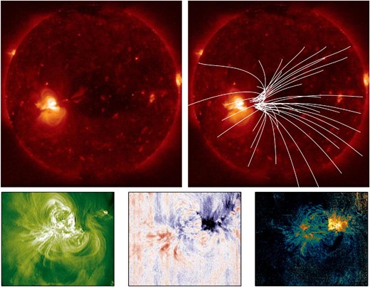
Top left: XRT Al-poly/Open image of AR 10978 as it approached disk center in 2007 December. Top right: PFSS extrapolation of the open field around the AR. Bottom left: EIS Fe xii 192.394 Å spectral image of the AR. Bottom center: Doppler velocity map derived from the EIS Fe xii 192.394 Å data. Bottom right: Non-thermal velocity map derived from the EIS Fe xii 192.394 Å data following the method of Brooks and Warren (2016). Note that the open field in the extrapolation anchors close to the upflows but they are not necessarily co-spatial. We discuss the importance of understanding the magnetic topology in the text. (Color online)
EIS line profiles often show weak asymmetries in the blue wing (Hara et al. 2008a), which have been linked to jets and spicules in the chromosphere (De Pontieu et al. 2009). The apparent motions seen in XRT data were also sometimes observed to propagate along fan-like loops at the edges of active regions, and spicules have again been suggested as the driver (McIntosh & De Pontieu 2009). A large amount of work has been done determining whether these motions are the result of flows or waves or indeed waves in a flow. For a recent review of this topic see, e.g., Wang (2016). EIS observations of the temperature dependence of the upflows, however, showed that they are most consistently seen above 1 MK, and redshifted downflows are seen in the fans at lower temperatures (Warren et al. 2011b; Young et al. 2012). Measurements of the blue wing asymmetries are consistent with this. The asymmetries can reach at least 100 km s−1 in the upflows (Bryans et al. 2010; Peter 2010; Tian et al. 2011a, 2011b), but are weaker below 1 MK and increase as a function of temperature (Brooks & Warren 2012). The blue wing enhancements are seen on transient time scales (∼5 min) in the coronal lines, supporting an association with dynamic events, but are not observed below 1 MK (Ugarte-Urra & Warren 2011). When blue wing asymmetries are seen in chromospheric lines the results are mixed. He et al. (2010) observed chromospheric jets at the base of upflows in He ii, whereas Madjarska, Vanninathan, and Doyle (2011) found that asymmetries in Hα do not appear to be located in the coronal upflow regions.
To establish a direct link between these flows and the slow solar wind we can also examine the plasma properties measured remotely and compare them to corresponding measurements made in situ in the near-Earth environment. Taking advantage of the FIP effect, Brooks and Warren (2011) examined the plasma composition in the upflows of AR 10978. They found that an enhanced slow-wind composition persistently flowed from the AR for the full five days of their observations. In fact, the measurements made when the flows from the western side of AR 10978 were directed towards Earth were found to be consistent with values obtained in situ several days later by the ion composition spectrometer SWICS on the ACE spacecraft. Brooks and Warren (2012) performed a similar analysis for the asymmetric high-speed component of the flows and found that they also showed an enhanced slow-wind composition, suggesting that the high-speed and bulk flows may share a common formation mechanism. Furthermore, Culhane et al. (2014) examined Fe/O ratios obtained by SWICS, and found evidence of a response to AR 10978’s passage through disk center. In a study of a separate AR, Slemzin et al. (2013) also provided support for a connection by linking measurements made in situ by ACE and other observatories to the AR source using ballistic back-mapping and a PFSS model.
These observations have inspired new theoretical thinking on the formation of the upflows, and whether the magnetic topology is such that they truly become outflows that connect to the heliosphere. From magnetic field extrapolations, Baker et al. (2009) found that the narrow corridors at the base of the upflows coincide with surface projections of quasi-separatrix layers (QSLs) in the corona. These are regions of strong gradients in magnetic connectivity, and are prime sites for processes such as interchange reconnection (Fisk et al. 1998) between the closed AR field and surrounding open, or distantly connected, field. If there is a nearby coronal hole, then in a sense this process is similar to other models of the source and formation of the slow wind, such as the S-web (web of separatrices) model (Antiochos et al. 2011), that do not involve ARs but describe interchange reconnection along coronal hole boundaries (Higginson et al. 2017).
Murray et al. (2010) have shown that the continual expansion of evolving ARs in coronal holes can drive and accelerate flows along the open field in the vicinity of separatrix surfaces. Del Zanna et al. (2011a) expanded this suggestion to propose a similar scenario of AR growth maintaining continuous reconnection across separatrices at the null point they located in the coronal magnetic field topology derived from potential and linear force-free field extrapolations. In this scenario, pressure gradients develop following reconnection between the cooler open-field lines and the hot loops of the AR core, and this appears to be consistent with numerical hydrodynamic simulations (Bradshaw et al. 2011). If an interchange mechanism is really operating in QSLs to drive the flows, it might also be possible to detect signatures of that process in radio measurements. Interestingly, Del Zanna et al. (2011a) did indeed find evidence of a correspondence between flow locations and radio noise storms.
So, the model of interchange reconnection at QSLs is beginning to produce a compelling picture of the flows. AR expansion and growth drive the interchange reconnection, which provides the mechanism to transfer slow-wind-composition plasma from closed AR loops to open field and expel the material. The flows are seen as propagating features in XRT movies and Doppler-shifted upflows in EIS data. Radio noise storms are indicative of the reconnection process. EIS elemental abundance measurements confirmed that the composition is enhanced as in the slow wind, and when the plasma has had time to travel to the Earth environment, in situ measurements of the composition are consistent with those measured with EIS.
There are, however, some issues that cloud this interpretation. Most importantly, the magnetic field topology is not always consistent with this picture. Culhane et al. (2014), for example, found that AR 10978—the region that showed slow wind compositional signatures at ACE—was completely covered by a closed helmet streamer. Furthermore, in a study of seven ARs, Edwards et al. (2016) found that most of them did not have high-reaching or open field in the vicinity of the upflows. Only in one AR, adjacent to a coronal hole as in Sakao et al. (2007), was an outflow channel found. If an adjacent coronal hole is a prerequisite for the development of open field, then the upflows may not be true outflows in general; see also Fazakerley, Harra, and van Driel-Gesztelyi (2016). Boutry et al. (2012) also found that a sizeable fraction of mass flux (1/5 in their example) propagated away from the upflow area along long loops that connected to distant ARs. So not all of the outwardly propagating mass flux necessarily escapes to interplanetary space.
Culhane et al. (2014) and Mandrini et al. (2015) have addressed the example of AR 10978 with a detailed topological study using a PFSS model. They found that closed-field plasma could escape along a novel pathway via a two-step reconnection process. First, the AR closed loops reconnected with large-scale network field, producing long loops that anchored close to the high-latitude open field associated with a northern coronal hole where a high-altitude null point was also located. AR plasma traveled along these new loops, and in a second step, interchange reconnection with the open field released the plasma. This suggested that closed-field plasma can escape into the solar wind, even when it appears unlikely.
Such complex escape pathways may not be necessary in general, however. van Driel-Gesztelyi et al. (2012) showed how the presence of two bipolar ARs on disk could create a quadrupolar magnetic configuration allowing the presence of a null point where AR plasma can be channeled into the slow wind. Taking a different approach, Brooks, Ugarte-Urra, and Warren (2015) designed a novel observing sequence to scan the entire solar disk with EIS, and combined the observations with a PFSS model to try to locate all regions of open field that show upflows with a slow-wind composition. They found numerous areas of slow-wind-composition outflow on open magnetic field. Despite a downward revision of the outflow mass flux compared to Sakao et al. (2007), based on spectroscopic densities and velocities, they found that the outflow regions could account for most of the mass-loss rate of the solar wind as benchmarked against ACE measurements.
There are, of course, alternative slow-solar-wind models that may provide an explanation for the outflows. Theories that do not involve loop opening, such as wave/turbulence models (Cranmer 2012), have difficulty explaining how enhanced composition plasma is supplied to the slow wind, since the most widely studied models of the FIP effect assume that plasma must be confined for some time in order for the fractionation mechanism to operate (Laming 2004, 2012). Leaving aside the models, EIS measurements show that one can have slow-wind-composition plasma on open magnetic field. Whether this is proof that loops have been opened, or is a new clue to understanding wave and FIP effect models, remains to be seen. In any case, Hinode has shown that it is no longer correct to state that the slow wind only has the same composition as the closed-field corona. In fact, many areas of open field have the same composition.
10 Future prospects
During the last eleven years solar physics has made remarkable progress and Hinode has been a key contributor to these advances, as is amply demonstrated by the earlier sections of this review paper. In this section we consider the prospects for progress in the next eleven years. To a large extent any speculation on future advances is based on extrapolating from the progress that has occurred in past years, while taking into account the influence of (observational and/or theoretical) instruments already under development or planned. The biggest uncertainty for such an exercise is posed by the emergence of new ideas that can advance the field in unpredictable ways. In addition, any predictions will be colored by the experience and interests of the person making them. Nonetheless, it is abundantly clear that, barring serious technical problems, Hinode will continue to play an important role in the years to come, in particular when acting together with other resources. Many past investigations have already made use of Hinode data obtained in conjunction with other space missions such as SOHO (Domingo et al. 1995), SDO (Pesnell et al. 2012), and more recently IRIS (De Pontieu et al. 2014b), as well as with various ground-based telescopes, such as the Dunn Solar Telescope (DST; Dunn & Smartt 1991), the German Vacuum Tower Telescope (VTT; von der Lühe 1998), the Swedish Solar Telescope (SST; Scharmer et al. 2003), the Goode Solar Telescope (GST; Goode et al. 2010), GREGOR (Schmidt et al. 2012), and very recently with ALMA (Shimojo et al. 2017b). In future we expect a bonanza from joint observations with projects under development, such as DKIST (Tritschler et al. 2016), the Parker Solar Probe (Fox et al. 2016), and Solar Orbiter (Müller et al. 2013), but also with, e.g., the SUNRISE mission (Solanki et al. 2010, 2017; Barthol et al. 2011) during its upcoming third flight.
Let us start a brief tour of some of the sub-fields of solar physics by considering the solar interior. There, interest has focused on differential rotation, meridional circulation, and turbulent convection, i.e., on the key flows driving the global solar dynamo and hence leading to the production of the Sun’s large-scale magnetic field that forms sunspots and active regions. Considerable progress has been achieved over the last decade (Gizon et al. 2010; Hanasoge et al. 2016; Howe 2016; Zhao & Chen 2016). However, considerable inconsistencies and gaps in our knowledge exist, particularly of the strength of the turbulent convection (Hanasoge et al. 2012; Greer et al. 2015), and quite generally of the flows near the poles. In addition, the structure and magnitude of these flows in the lower convection zone are rather poorly known. This is particularly true for the meridional circulation, where it is even unclear at which depth the return flow (i.e., from pole to equator) takes place and whether there is a single meridional circulation cell or multiple cells at different depths (Zhao et al. 2013; Rajaguru & Antia 2015).
A number of advances have been made in understanding the global solar dynamo in the last decade. Three-dimensional simulations of the entire convection zone have progressed considerably, allowing direct numerical simulations of a dynamo residing in the convection zone (e.g., Käpylä et al. 2016). In parallel, the Babcock–Leighton-type dynamo, with the surface field playing a key role (Cameron & Schüssler 2015), has made a remarkable comeback. The long-standing problem of maintaining a large-scale field even in the presence of a high Reynolds number has recently been solved by Hotta, Rempel, and Yokoyama (2016). The importance of polar fields for the global dynamo has been clarified by, e.g., Wang and Sheeley (2009), while the important role of sunspot or active region tilt angles for building up the polar fields at activity minimum has also been demonstrated (Dasi-Espuig et al. 2010, 2013; Jiang et al. 2014).
One of the major breakthroughs of the last decade has been the demonstration that a small-scale turbulent dynamo is viable under “realistic” solar photospheric conditions (Vögler & Schüssler 2007). More recent simulations with lower numerical viscosity have been carried out by Rempel (2014) and Hotta, Rempel, and Yokoyama (2015), and the results of such simulations are by now well established—see also the reviews by Brandenburg, Sokoloff, and Subramanian (2012) and Borrero et al. (2015). Observational support has come largely from data obtained with Hinode/SOT. Such data have demonstrated that there is no variation of the magnetic flux in the inter-network over the solar cycle (Buehler et al. 2013; Lites et al. 2014; Jin & Wang 2015), and have also shown to high accuracy that the SOT-SP high-resolution observations are consistent with the results of small-scale dynamo simulations (Danilovic et al. 2010b, 2016a).
In spite of these advances, our understanding of the dynamo remains rather incomplete. An important open question is the location of the global solar dynamo (besides the solar surface): Does it reside in the overshoot layer below the convection zone, in the lower convection zone, throughout the convection zone, or in the shear layer near the solar surface?
To make progress in these topics it will be necessary to observe the Sun from new vantage points with an instrument measuring velocities and taking vector magnetograms. It is hoped that the deeper parts of the convection zone can be better probed by observing the p-mode oscillations from two different directions (with a technique dubbed stereoscopic helioseismology). With regard to the surface magnetic field, so far the most detailed maps of the magnetic field at the solar poles have been made by using Hinode data (see subsection 4.1). Only high-resolution observations from outside the ecliptic will be able to go beyond what Hinode has achieved. Such observations will be provided by the PHI instrument (Solanki et al. 2015) on Solar Orbiter from heliographic latitudes higher than 30° during its extended mission phase. Nonetheless, continuing regular coverage of the polar fields by Hinode also remains important for the future, not just to bridge the time until Solar Orbiter reaches higher latitudes, but also as a regular complement after that date (as Solar Orbiter will have only two high-latitude passes every 150 d).
When probing the physics of the photosphere and the chromosphere, the quest for high resolution will continue. Hinode made the important point that a telescope in a seeing-free and stable environment such as space will lead to basic discoveries and novel results that telescopes with two or three times the diameter have difficulty attaining from the ground. Thus, with its 50 cm Hinode/SOT has only half the diameter of the SST, which was already operational at the time of Hinode’s launch, and roughly a third of that of the GST and GREGOR, which started observing later. And yet Hinode was the first to discover a whole range of phenomena and provide answers to a whole string of questions (see sections 3 and 7). With its seeing-free, low-noise spectro-polarimetry, Hinode will continue to provide outstanding data for future studies.
The contribution of inversion techniques (see sub-subsection 3.1.1) to Hinode’s success in photospheric and chromospheric physics should not be underestimated. They play the key role in deducing the atmospheric parameters, in particular the line-of-sight velocity and the magnetic vector, from the observations. One such advanced technique is the so-called coupled 2D inversion of van Noort (2012) and van Noort et al. (2013). Such inversions provide the structure of the photosphere (and if fed the appropriate data also of the chromosphere) after the removal of the PSF of the instrument (Lagg et al. 2014; Buehler et al. 2015; Danilovic et al. 2016a). A similar outcome is achieved with deconvolutions (even if in theory they are somewhat less ideal; Quintero Noda et al. 2015). Both techniques enhance the sharpness of the images (at each wavelength and polarization) significantly and work best when the PSF is well known and stable, a major plus for a space-borne observatory, giving it an edge over larger telescopes on the ground. An extension of inversions to the chromosphere requires taking non-LTE effects into account (see below).
With the largest and best current telescopes we are starting to resolve the photospheric horizontal photon mean free path (in the plane-parallel approximation) of 50–100 km. This implies that as larger telescopes, such as DKIST and EST, start obtaining data close to their diffraction limits, true 3D radiative transfer will become increasingly important, not just for the chromosphere (Leenaarts et al. 2012, 2013, 2015) but also for the photosphere (Holzreuter & Solanki 2013, 2015). Nonetheless, the computations suggest that even below the horizontal mean free path we will continue to see ever smaller structures with increasing telescope size (although possibly at lower contrast), as long as we use the correct diagnostics (Judge et al. 2015).
Just like the telescopes, the post-focus instruments are also evolving rapidly. A critical shortcoming of almost all current instruments is that they cannot simultaneously cover the spectral and both spatial dimensions (i.e., they cannot instantaneously obtain a full spectrum in every pixel of an area on the Sun). However, this is necessary because solar features evolve rapidly, also over the time scales needed to complete spatial scans (e.g., when using slit spectrographs), or spectral scans (when using narrow-band imagers), so that the information obtained by such “standard” instruments is distorted. The solution to this fundamental issue is provided by integral-field units (IFUs) and, with a somewhat different approach, by their cousins—multi-slit spectrographs and image slicers. These instruments are now beginning to come of age. They have the clear advantage of imaging an area (or scanning it very rapidly in the case of multi-slit spectrographs and image slicers) while simultaneously recording the undistorted spectrum. They will likely become central instruments for solar observations in the coming decade. Their advantages will be particularly evident for studies of complex dynamic phenomena. Different types of IFUs are being developed for solar use, with those based on microlenses and on optical fibers having been developed the furthest. Key challenges are to get reliable polarimetric data and a sufficiently large FOV (i.e., a sufficiently large number of both spatial and spectral pixels).
In spite of its rather limited chromospheric capabilities, Hinode produced vast advances in our knowledge of this relatively poorly studied layer of the solar atmosphere (e.g., sections 2 and 5, and subsection 7.2). The lack of spectroscopic and polarimetric capabilities in a chromospheric spectral line, i.e., the missing capability to measure velocities and the magnetic field in the chromosphere, hindered Hinode from taking even larger strides. The importance of such capabilities has been amply demonstrated from the ground. In particular, the development of various diagnostics of the chromospheric magnetic field (e.g., Stokes spectro-polarimetry in the He i 10830 Å triplet and the Ca ii IR triplet) along with the corresponding inversion techniques has great potential (Solanki et al. 2003; Lagg et al. 2004, 2007; Socas-Navarro 2005; Kuckein et al. 2009, 2012; Xu et al. 2010, 2012; Kleint 2017); see also de la Cruz Rodríguez and van Noort (2017) and references therein. However, the full potential of such data has not been tapped so far, partly because of the need for extremely low-noise data, due to the small chromospheric Stokes signals.
In the coming years this will change and the chromospheric magnetic field will be much more commonly measured, partly due to the excellent capabilities of GREGOR, SST, GST, SUNRISE III (the third flight of SUNRISE; Barthol et al. 2011), DKIST, and CLASP II (the second flight of CLASP; Kano et al. 2012), ideally observing together with SOLAR-C_EUVST and ALMA. Particularly effective will be IFUs with a reasonable FOV coupled with large-aperture telescopes. This combination will allow us to probe in detail the highly dynamic, magnetically dominated chromosphere in real time, with the IFU providing 3D data cubes at a high cadence, while the large-aperture telescope will provide sufficient photons to obtain the necessary signal-to-noise ratio.
Advances in the inversion of chromospheric spectral lines will also play an important role in probing the solar chromosphere in the future (de la Cruz Rodríguez & van Noort 2017). Non-LTE inversion codes have now been developed that takes different approaches to make this difficult problem more manageable (e.g., Socas-Navarro et al. 2015; Milić & van Noort 2018; de la Cruz Rodríguez et al. 2019).
An important new window on the solar chromosphere that complements the diagnostics in the UV, visible, and infrared is being opened by ALMA (Wedemeyer et al. 2016). Partly, this is because millimeter-wavelength radiation reacts differently to the thermal properties of the gas than the radiation at shorter wavelengths. ALMA is by far not the first instrument to sample the Sun at millimeter wavelengths, but it does so at around an order of magnitude higher spatial resolution. First solar science observations, with a spatial resolution on the order of 1″–2″, have finally been obtained in 2016 December. A number of surprises are expected, as already investigations with the lower-quality commissioning data have provided new insights (e.g., Iwai et al. 2017; Shimojo et al. 2017a).
Many of the big steps taken by Hinode in uncovering the physics of the solar photosphere and chromosphere have been accompanied and aided by MHD simulations, which have undergone an amazing evolution over the lifetime of the Hinode mission. Recent large-scale MHD simulations produce realistic-looking (i.e., highly irregular) active regions with sunspots, including sizeable penumbrae, in particular between opposite-polarity sunspots [Rempel and Cheung (2014), M. Rempel (2017), private communication] in addition to excellent representations of smaller magnetic features and convection cells. Another nice example is that the combination of measured surface velocities and MHD simulations led to the conclusion that in the uppermost 2 × 10⁴ km of the convection zone, active regions rise with a speed similar to convective upflows, but much slower than predicted by the buoyant rise of thin magnetic flux tubes (Birch et al. 2016).
The future will likely see further rapid improvements in MHD simulations. They will include the coverage of larger heights (and depths) and of longer intervals of time. A number of radiation-MHD codes already provide a relatively viable coverage of physical processes in the solar convection zone and photosphere, e.g., Stagger (Nordlund & Galsgaard 1995),18 MuRAM (Vögler et al. 2005), CO5BOLD (Freytag et al. 2002), and Bifrost (Gudiksen et al. 2011). In addition, MuRAM, Bifrost, and Pencil (Brandenburg & Dobler 2002) have been used to model the corona. However, only Bifrost includes non-LTE radiative transfer, needed to properly represent the chromosphere. Other codes will also need such an extension before they can properly simulate all layers of the solar atmosphere.
One major aim of future simulations should be to follow the evolution of whole active regions from their initiation deep in the solar interior right up to their decay, covering processes such as the formation and evolution of sunspots, prominences, bright coronal loops, jets, flares, CMEs, etc. This may partly be possible simply by increasing computational power (e.g., larger and deeper boxes and longer time series), while a more realistic realization of the chromosphere and corona likely requires better treatment of the physical processes already included in current simulations, such as improved radiative transfer (mainly in the chromosphere), or further departures from a purely MHD treatment. One hint that current radiation-MHD simulations are in need of further improvement (in spite of their great success) is given by the fact that although the simulations with Bifrost have had many remarkable successes, the widths of prominent chromospheric spectral lines, such as the Mg ii h and k lines, are considerably narrower than observed (Leenaarts et al. 2013). It is as yet unclear if this is due to insufficient resolution or due to missing physics. In any case, departures from pure MHD have been included in the MANCHA3D code initially developed by Khomenko and Collados (2006), including ambipolar diffusion, the Hall effect, and the battery effect, while Martínez-Sykora, De Pontieu, and Hansteen (2012) incorporated the Hall effect and ambipolar diffusion into a 2D version of Bifrost. Hence, these codes take into account that the coupling between ions, electrons, and neutrals may not be perfect in the chromosphere.
Probably the biggest open question in coronal physics concerns how the solar corona is heated. This question may possibly be too broad to be answered in a simple way, and needs to be broken down into a number of sub-questions. For example, how are magnetic field lines energy-loaded in the photosphere and solar interior? How is this energy transported to the upper solar atmosphere? Where and by which processes is the energy released? These questions, along with many others, were to be studied by the original SOLAR-C project, which would have been the first mission to cover all layers of the solar atmosphere (at high spatial and temporal resolution). The downselected SOLAR-C_EUVST (which is similar to the LEMUR instrument proposed for the original SOLAR-C; Teriaca et al. 2012b) will not be able to study the critical lower atmospheric layers, where the energy loading happens, but will sample most of the rest of the atmosphere, making it a powerful tool to address coronal heating. In the meantime, the Solar Orbiter coronal instruments Spectral Imaging of the Coronal Environment (SPICE; Fludra et al. 2013) and Extreme Ultraviolet Imager (EUI; Halain et al. 2012) will provide some of the necessary high-spatial-resolution spectrometric (reaching 0|${^{\prime\prime}_{.}}$|8) and imaging (reaching 0|${^{\prime\prime}_{.}}$|2) data, although only for a short period of time around perihelion of each orbit and without covering the solar atmosphere to the same extent. Nonetheless, there will also remain a strong need for instruments that study the corona on a permanent basis. Here, EIS and XRT on Hinode will remain mainstays for years to come, as providers of regular high-quality coronal spectroscopy and X-ray imaging.
Two mechanisms (or families of mechanisms) are the most widely considered for heating the corona: (1) nanoflares—heating by release of magnetic energy at tangential discontinuities produced by braiding of magnetic field lines that are constantly being randomly transported by photospheric turbulent convection (Parker 1988); (2) waves—heating by dissipation of MHD waves transported along magnetic field lines connecting the solar interior to the corona, see, e.g., De Moortel and Browning (2015), who review not just wave heating models of the corona. Recently, yet another mechanism, or possibly a variant of the first mechanism, as it also involves magnetic reconnection, has been proposed. Chitta et al. (2017) noticed in data taken by the IMaX instrument (Martínez Pillet et al. 2011) during the second flight of SUNRISE that often both magnetic polarities are present at a given footpoint of a coronal loop, a dominant polarity (well visible also in low-resolution magnetograms) and a minor polarity (not clearly seen in lower-resolution data). These authors also found that the opposite polarities were canceling at the footpoints of particularly bright loops (cf. Chitta et al. 2018). They proposed that the reconnection associated with the canceling flux heats and accelerates gas that then fills the entire loop—small jets of gas at chromospheric temperatures were seen by the SuFI instrument on SUNRISE (Gandorfer et al. 2011) emanating from the locations of flux cancelation—making it bright in EUV radiation (cf. Priest et al. 2018). Although having evidence for a new mechanism is exciting and may help overcome some of the problems facing the classical mechanisms, it is still unknown how common such minor opposite polarity features are and how often they cancel with the dominant polarities at the footpoints of coronal loops. In the coming years, new very high resolution observations of magnetic footpoint motions (necessary to determine how effectively field lines get braided) and of cancelation between opposite magnetic polarities at loop footpoints will help decide how efficient different mechanisms for heating the corona are.
Besides high-spatial-resolution spectra covering the full range of coronal and transition region temperatures, coronal magnetic field measurements are among the data needed most to gain an understanding of coronal heating. There have been a number of advances on this front in past years, with both radio (Iwai & Shibasaki 2013; Bogod & Yasnov 2016) and infrared (Lin et al. 2004) observations contributing, but the situation remains unsatisfactory. A major step forward is expected from DKIST, whose off-axis, low-scattered-light design along with its large aperture and infrared instrumentation could make it an ideal instrument for high-resolution studies of coronal magnetic fields. Just as important as the measurements will be improved methods to interpret them (e.g., tomography, either based on changing lines of sight due to solar rotation or, preferably, making use of stereoscopy from multiple vantage points). Since the coronal gas is optically thin and very inhomogeneous in terms of temperature and density, it will be very difficult to get the magnetic field’s structure throughout the corona. Here, observations from different vantage points will help.
At the same time, magnetic field extrapolations will continue to improve (Wiegelmann & Sakurai 2012; Wiegelmann et al. 2014). Over the past decade modeling has progressed from initially mainly potential-field extrapolations to mainly NLFFF extrapolations, as vector magnetograms have become increasingly available and codes have improved (DeRosa et al. 2015). However, such methods have their limitations, in particular when predicting the current density and free energy, as shown by Peter et al. (2015). Therefore, in the future we expect such methods to evolve further, towards data-driven magnetostatic solutions and MHD models [see Inoue (2016) and references therein]. Such solutions have the advantage of taking into account the influence of forces, such as those exerted by gas pressure gradients, not just in the lower atmospheric layers where plasma β is globally larger than unity, but also in those parts of the upper atmosphere where β ≥ 0.05. Making increasing use of more regular future chromospheric magnetic field measurements (obtained above the plasma β = 1 surface) to constrain extrapolations could also lead to an improvement. This will, however, require very low noise chromospheric spectro-polarimetric measurements and reliable inversions. In particular, it will require a way of determining the height to which the chromospheric measurements refer.
Overcoming the challenges facing coronal magnetic field measurements will require a concerted approach involving the combination of the various available direct (e.g., polarimetry) and indirect (intensity, stereoscopy) diagnostics with data-driven modeling (e.g., extrapolations). First steps in this general direction have been taken by Kramar et al. (2013, 2016) and Chifu, Inhester, and Wiegelmann (2015); cf. Gibson et al. (2016).
In summary, the last decade has seen a huge amount of progress, much of it due to the outstanding observations obtained by Hinode, as the earlier sections of this review indicated. Building on this we expect many more significant advances in the coming decade. Hinode itself will continue to contribute strongly with new observations (as well as with the data already in its sizeable archive), increasingly helped by new instruments and missions as well as by advances in theory and modeling. We await another exciting decade of science based on Hinode observations.
Acknowledgments
Hinode is a Japanese mission developed and launched by ISAS/JAXA, with NAOJ as a domestic partner and NASA and STFC (UK) as international partners. It is operated by these agencies in cooperation with ESA and NSC (Norway). P. Antolin has received funding from the UK Science and Technology Facilities Council and the European Union Horizon 2020 research and innovation program (grant agreement no. 647214) and his STFC Ernest Rutherford Fellowship (grant agreement no. ST/R004285/1). Numerical computations in subsection 6.1 were carried out on a Cray XC30 at the Center for Computational Astrophysics, NAOJ. He would like to thank I. De Moortel for her valuable comments on subsection 6.1. The work of L. Bellot Rubio was supported by the Spanish Ministerio de Economía, Industria y Competitividad through projects ESP2014-56169-C6-1-R and ESP2016-77548-C5-1-R, including a percentage from European FEDER funds, and by the European Commission’s FP7 Capacities Programme under the SOLARNET project (grant agreement 312495). The work of D. Brooks was performed under contract to the Naval Research Laboratory and was funded by the NASA Hinode program. L. Fletcher was supported by STFC grant number ST/L000741/1 and by the European Community’s Seventh Framework Programme (FP7/2007–2013) under grant agreement no. 606862 (F-CHROMA), and gratefully acknowledges support from the organizers of the Hinode-10 meeting. A. S. Hillier was supported by his STFC Ernest Rutherford Fellowship grant number ST/L00397X/2. T. M. D. Pereira was supported by the European Research Council under the European Union’s Seventh Framework Programme (FP7/2007–2013)/ERC grant agreement no. 291058. T. Sakao would like to thank E. DeLuca, M. Weber, K. Reeves, and L. Golub for their careful reading and comments on subsection 2.3. The work of T. Sakurai was supported by JSPS KAKENHI grant numbers JP15K05034 and JP15H05816. The work of D. Shiota and M. Shimojo was partly carried out at the NAOJ Hinode Science Center, which is supported by the Grant-in-Aid for Creative Scientific Research “Basic Study of Space Weather Prediction” from MEXT, Japan (17GS0208, Head Investigator: K. Shibata), generous donations from Sun Microsystems, and NAOJ internal funding. The contribution of S. K. Solanki has received funding from the European Research Council (ERC) under the European Union Horizon 2020 research and innovation program (grant agreement no. 695075) and has been supported by the BK21 plus program through the National Research Foundation (NRF) funded by the Ministry of Education of Korea. A. C. Sterling was supported by funding from the Heliophysics Division of NASA’s Science Mission Directorate through the Heliophysics Guest Investigators (HGI) Program; he thanks R. L. Moore and N. K. Panesar for careful reading of subsection 7.2. The work of Y. Su was supported by the NSFC grant no. 11473071, the One Hundred Talent Program of CAS, and by the Youth Fund of Jiangsu no. BK20141043. She is grateful to B. Kliem for his valuable comments on subsection 8.1. S. K. Tiwari would like to thank R. L. Moore for helpful comments on subsection 7.1. His research was supported by an appointment to the NASA Postdoctoral Program at the NASA Marshall Space Flight Center, administered by the Universities Space Research Association under contract with NASA. He gratefully acknowledges his current support by NASA contracts NNG09FA40C (IRIS) and NNM07AA01C (Hinode). The work of S. Toriumi was supported by JSPS KAKENHI grant numbers JP16K17671 and JP15H05814. Finally, all the authors would like to thank our coauthor Ted Tarbell, who passed away in 2019 April, for his contributions to this article and to the entire Hinode project.
Appendix. List of abbreviations
The page numbers show the first appearance or most essential description in the text.
ACE/SWICS: Solar Wind Ion Composition Spectrometer on ACE, 95
ACE: Advanced Composition Explorer, 95
AOCS: Attitude and Orbit Control System of Hinode, 5
BFI: Broad-band Filtergraphic Imager of Hinode/SOT, 6
CLASP: Chromospheric Lyman-Alpha Spectro-Polarimeter, a rocket experiment, 99
CO: Hinode Chief Observer, 5
CoMP: Coronal Multichannel Polarimeter of U.S. National Solar Observatory at Sacramento Peak, 40
CP: Hinode Chief Planner, 5
CT: Correlation Tracker of Hinode/SOT, 6
DKIST: Daniel K. Inouye Solar Telescope in Hawaii, 19, 97
DST: Dunn Solar Telescope of U.S. National Solar Obser-vatory at Sacramento Peak, 19, 97
EIS: Hinode EUV Imaging Spectrometer, 4, 13
EST: European Solar Telescope, planned to be located in the Canary Islands, 19
EUNIS: Extreme Ultraviolet Normal Incidence Spectro- graph, a rocket experiment, 50
FG: Filtergraphs of Hinode/SOT, 6
FOXSI: Focusing Optics X-ray Solar Imager, a rocket experiment, 50
FPP: Focal Plane Package of Hinode/SOT, 6
GOES/SXI: Solar X-ray Imager on GOES, 62
GOES: Geostationary Operational Environmental Satellite, 12, 62
GST: Goode Solar Telescope (New Solar Telescope) at Big Bear Solar Observatory, New Jersey Institute of Technology (NJIT), 97
Hi-C: High Resolution Coronal Imager, a rocket experi-ment, 55
HOP: Hinode Operation Plan, 6
HXT: Yokhoh Hard X-ray Telescope, 82
IRIS: Interface Region Imaging Spectrometer, 29
LEMUR: Large European Module for Solar Ultraviolet Research, a proposal for SOLAR-C, 100
MDP: Mission Data Processor of Hinode, 6
NFI: Narrow-band Filtergraphic Imager of Hinode/SOT, 6, 8
NST: New Solar Telescope (Goode Solar Telescope) at Big Bear Solar Observatory, New Jersey Institute of Technology (NJIT), 65
NuSTAR: Nuclear Spectroscopic Telescope Array, 50
OTA: Optical Telescope Assembly of Hinode/SOT, 6
PMU: Polarization Modulation Unit of Hinode/SOT, 6
RHESSI: Reuven Ramaty High-Energy Solar Spectroscopic Imager, 82
SDO/AIA: Atmospheric Imaging Assembly on SDO, 11
SDO/HMI: Helioseismic Magnetic Imager on SDO, 15
SDO: Solar Dynamics Observatory, 11
SMEI: Solar Mass Ejection Imager, 33
SMM: Solar Maximum Mission, 75
SO/EUI: Extreme Ultraviolet Imager on Solar Orbiter, 100
SO/PHI: Polarimetric and Helioseismic Imager on Solar Orbiter, 97
SO/SPICE: Spectral Imaging of the Coronal Environment on Solar Orbiter, 100
SOHO/CDS: Coronal Diagnostic Spectrometer on SOHO, 85
SOHO/EIT: Extreme-Ultraviolet Imaging Telescope on SOHO, 59
SOHO/LASCO: Large-Angle and Spectrometric Corona-graph on SOHO, 33
SOHO/MDI: Michelson Doppler Imager on SOHO, 15
SOHO/SUMER: Solar Ultraviolet Measurements of Emitted Radiation experiment on SOHO, 40
SOHO: Solar and Heliospheric Observatory, 15
SOLAR-C_EUVST: SOLAR-C Extreme Ultra-Violet High- Throughput Spectroscopic Telescope, 99
SOT: Hinode Solar Optical Telescope, 4, 6
SP: Spectro-polarimeter of Hinode/SOT, 6, 8
SSOC: Sagamihara Spacecraft Operation Center, 5
SST: Swedish Solar Telescope in La Palma, 17
STEREO/COR2: Outer Coronagraph on STEREO, 33
STEREO/SECCHI-EUVI: Extreme Ultraviolet Imager in Sun Earth Connection Coronal and Heliospheric Investigation (SECCHI) instrument suite of STEREO, 59
STEREO: Solar-Terrestrial Relations Observatory, 33
SUNRISE/IMaX: Imaging Magnetograph Experiment on the SUNRISE balloon-borne telescope, 16, 100
SUNRISE/SuFI: SUNRISE Filter Imager, 100
SWG: The Hinode Science Working Group, 4
SXT: Yokhoh Soft X-ray Telescope, 3
TRACE: Transition Region and Coronal Explorer, 59
UFSS: Ultra-Fine Sun Sensor of Hinode, 5
USC: Uchinoura Space Center, ISAS/JAXA, 3
VLS: Visible Light Shutter of Hinode/XRT, 7
VTT: German Vacuum Tower Telescope in Tenerife, 19
XRT: Hinode X-Ray Telescope, 4, 10
Footnotes
For details, see 〈http://www.isas.jaxa.jp/home/solar/guidance/〉.
Such as 〈http://darts.isas.jaxa.jp/solar/hinode/〉.
Available at 〈http://xrt.cfa.harvard.edu/resources/documents/XAG/XAG.pdf〉.
EIS Software Notes are available online at 〈https://hesperia.gsfc.nasa.gov/ssw/hinode/eis/doc/eis_notes/〉.
The most recent report on the Next Generation Solar Physics Mission (NGSPM) by the NGSPM Science Objectives Team of NASA, JAXA, and ESA can be found at 〈http://hinode.nao.ac.jp/SOLAR-C/SOLAR-C/Documents/NGSPM_report_170731.pdf〉.
The field strength distribution in the network peaks at 1.4 kG, as expected for strong flux tubes—see figure 9 in Orozco Suárez and Bellot Rubio (2012).
These bubbles, also observed by Otsuji et al. (2007), are thought to represent the largest magnetic loops emerging in the quiet Sun. Instead of two roundish footpoints, they show extended feet with crescent shapes.
Actually, some of the ephemeral regions detected in previous studies could have been clusters of unresolved inter-network magnetic elements.
Note that not all magnetic flux exists in the form of large patches; a small fraction of magnetic flux is distributed in the range of smaller patches. The magnetic flux associated with those small patches is observed in inter-network fields in the polar regions (Lites et al. 2014).
For the solar observation target identification convention, see Leibacher et al. (2010).
References
Author notes
Present address: Department of Mathematics, Physics and Electrical Engineering, Northumbria University, Newcastle upon Tyne, NE1 8ST, UK.
Present address: Rosseland Centre for Solar Physics, University of Oslo, P.O.Box 1029, Blindern, NO-0315 Oslo, Norway.
Present address: PMOD/WRC, Dorfstrasse 33, CH-7260 Davos Dorf, Switzerland ETh-Zürich, HIT building, Hönggerberg, Switzerland.
Deceased on 2019 April 11.
Present address: Institute of Space and Astronautical Science, Japan Aerospace Exploration Agency, 3-1-1 Yoshinodai, Chuo-ku, Sagamihara, Kanagawa 229-5210, Japan
Present address: NASA Goddard Space Flight Center, Code 671, Greenbelt, MD 20771, USA
