


Abstract
The structure of the photospheric vector magnetic field below a dark filament on the Sun is studied using the observations of the Spectro-Polarimeter attached to the Solar Optical Telescope onboard Hinode. Special attention is paid to discriminating between two suggested models, a flux rope or a bent arcade. “Inverse polarity” orientation is possible below the filament in a flux rope, whereas “normal polarity” can appear in both models. We study a filament in the active region NOAA 10930, which appeared on the solar disk during 2006 December. The transverse field perpendicular to the line of sight has a direction almost parallel to the filament spine with a shear angle of 30°, the orientation of which includes the 180° ambiguity. To know whether it is in the normal orientation or in the inverse one, the center-to-limb variation is used for the solution under the assumption that the filament does not drastically change its magnetic structure during the passage. When the filament is near the east limb, we found that the line-of-site magnetic component below the filament is positive, while it is negative near the west limb.This change of sign indicates that the horizontal photospheric field perpendicular to the polarity inversion line beneath the filament has an “inverse-polarity”, which indicates a flux-rope structure of the filament supporting field.
1 Introduction
Dark filaments or prominences are one of the most impressive objects observed by the optical Hα spectral line in the solar atmosphere (reviews in, e.g., Parenti 2014; Mackay et al. 2010; Tandberg-Hanssen 1995; Hirayama 1985). Cold heavy matter stays above the surface at an altitude of up to 100 Mm surrounded by hot coronal plasma. As suggested by the occurrence above the magnetic polarity inversion lines (PILs; Babcock & Babcock 1955), they are considered to be supported by the magnetic field opposing the gravity.
Numbers of theoretical studies have been conducted on the magnetic structure of filaments. Kippenhahn and Schlüter (1957) suggested that the cool material is stored at the dips near the top of the bent arcade fields because of its own weight. In another model proposed by Kuperus and Raadu (1974), the filament material is stored at the lower dips inside a flux rope above the PIL. In the Kippenhahn–Schlüter model, the transverse magnetic component crossing the filament has a “normal” polarity, i.e., the orientation of the field is from the positive to the negative local vertical polarities, while it is in the opposite direction, i.e., an “inverse” polarity, in the Kuperus–Raadu model.
Studying the equilibrium structure is not only important by itself but is also interesting for understanding a filament eruption, which is frequently followed by a large flare and a coronal mass ejection. In some observations, a slow evolution is found before an eruption (Feynman & Martin 1995; Chifor et al. 2006; Nagashima et al. 2007; Isobe & Tripathi 2006). This is considered to be a manifestation of the approaching process to the de-stabilization or the loss of equilibrium. In the model by Forbes and Isenberg (1991), the equilibrium state evolves slowly in response to, e.g., the surface motion (e.g., Kaneko & Yokoyama 2014). Through this evolution, the magnetic pressure force of the fields below a flux rope finally overcomes the tension force of the overlying magnetic field lines that is pulling the rope back. Chen and Shibata (2000) extended this idea to become that the final de-stabilization is triggered by an emerging flux in the vicinity of a flux rope corresponding to a filament. In both these models, the final state just before an eruption has a flux rope in the corona. On the other hand, models in which the eruption appears from an arcade structure are also proposed. The stretching motion along the PIL with a converging motion enhances the magnetic pressure via the stretched axial field (Amari et al. 2000), leading to the triggering of an eruption. The observation of a filament’s magnetic structure is necessary to understand the feasibility of these proposed processes.
The magnetic fields of the prominences have been diagnosed using the spectro-polarimetric data of the optical spectral lines (a review of the early works is found in Leroy 1989). The magnetic fields are the results of the inversion based on the Hanle or Zeemann effects. The early observations revealed that the magnetic field has a strength of around 10 G, is mostly horizontal, and makes an acute angle of about 40° relative to the spine (Leroy 1989; Bommier & Leroy 1998; reviews in Mackay et al. 2010). Casini et al. (2003) obtained the first map of the vector field of a prominence. They found organized patches of magnetic field that were significantly stronger (up to 80 G) in the surrounding weak horizontal field.
To find the field structure of a filament, the measurement of the photospheric magnetic field is an indirect method but is relatively more precise than those in the filament itself. Using the detailed polarimetric measurements, Lites (2005) reconstructed the photospheric vector magnetic field below some narrow active region filaments in comparison with high-resolution Hα observations. He found a flux rope structure in the filaments, i.e., the photospheric field had an inverse polarity structure. López Ariste et al. (2006) also found bald patch structures in the bipoles in a filament channel as well as at the foot of its barbs. Okamoto et al. (2008, 2009) found an evolving magnetic field underneath an active region filament and concluded that its evolution is consistent with an emerging flux rope structure. Kuckein, Martínez Pillet, and Centeno (2012) conducted a multi-wavelength, multi-height study of the vector magnetic field of an active region filament and found that its inferred fields suggest a flux rope topology.
This study reports the magnetic structure beneath a filament in the photosphere that is observed by the Spectro-Polarimeter attached with the Solar Optical Telescope onboard the Hinode spacecraft, which is capable of observing the four Stokes components of the Fe i 6301.5 & 6302.5 Å doublet lines emanating from the photosphere. These spectro-polarimetric data are fitted by our developed code, MEKSY, based on the Milne–Eddington atmospheric model. As for the practical procedure of the measurement of the transverse magnetic component, there remains the fundamental difficulty of the 180° uncertainty. The approach described in this study uses the center-to-limb evolution of the Stokes-V signal to solve the 180° ambiguity in the azimuthal angle of the photospheric vector field below the filament (see also Bommier et al. 1981). This method assumes that the global magnetic structure of the filament is static during this period.
Based on the measurement in this study, we attempt to discuss the global structure of the filament. In the Kippenhahn–Schlüter bent-arcade model, the transverse magnetic component crossing or beneath the cool material has normal polarity. In the Kuperus–Raadu flux-rope model, the crossing field has inverse polarity. However, for the photospheric field, there are two possibilities for the orientation: first, if the flux rope is detached above the photosphere, low-height loops can connect in a normal manner, and the magnetic field close to the photosphere can have normal orientation; secondly, if part of the flux rope field lines cross the photoshpere, a so-called bald patch configuration appears close to the PIL in the photosphere, and an inverse orientation can be observed.
In the next section, the observation is described. The results are given in section 3 with corresponding discussions.
2 Observation and analysis
We used the data sets taken by the observations of active region NOAA 10930 (figure 1) during its passage on the solar disk from 2006 December 8 to 16. The square insets of panels (a) and (b) in figure 1 indicate the analyzed filament.
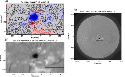
Active region NOAA 10930 on 2006 December 11. Color map in (a): LOS component of the magnetic field obtained by the Milne–Eddington fitting procedure from the Hinode SOT/SP observations. Red (blue) color indicates the positive (negative) polarity. The color plot is saturated at an absolute strength at 3 kG with dark blue (red) for negative (positive) field. Contours in (a) and gray-scale in (b): Brightness in the Hα band taken at the Big Bear Solar Observatory. The square insets in panels (a) and (b) indicate the filament studied in this paper. (c): The same data as (b) but in full observational field of view. The square line indicates the field of view of panels (a) and (b).
We used full-sun images in the hydrogen Hα band taken by the Global High-Resolution Hα Network, which consists of facilities at different global longitudes (Steinegger et al. 2001), as information on the chromospheric geometry of the filaments. In the analyzed period, data from the Big Bear Solar Observatory (BBSO; figures 1b and 1c) and the Meudon Observatory are available. We also used data taken by the Solar Magnetic Activity Research Telescope (SMART) at the Hida observatory of Kyoto University (UeNo et al. 2004) and by the Polarimeter for Inner Coronal Studies (PICS) of the Advanced Coronal Observing System (ACOS) at Mauna Loa Solar Observatory. The spatial resolution depends on the capability of the telescope for each image and also on the seeing level at the data acquisition. Unfortunately, the achieved resolutions are insufficient to resolve the fine structures in the chromospheric fibrils.
We analyzed the Stokes profiles obtained by the Spectro-Polarimeter (SP; Lites et al. 2013) attached with the Solar Optical Telescope (SOT; Ichimoto et al. 2008; Tsuneta et al. 2008; Shimizu et al. 2008; Suematsu et al. 2008) onboard the Hinode spacecraft (Kosugi et al. 2007) for the photospheric magnetic field. The SP obtains the profiles of two magnetically sensitive Fe i lines at 6301.5 Å and 6302.5 Å. Stokes IQUV data are obtained with a polarimetric accuracy of <0.1%. The sampling pixels are 0|${^{\prime\prime}_{.}}$|15 × 0|${^{\prime\prime}_{.}}$|16 in the normal-map mode and 0|${^{\prime\prime}_{.}}$|30 × 0|${^{\prime\prime}_{.}}$|32 in the fast-map mode. The spectral resolution (sampling) is 30 mÅ (21.5 mÅ). The field of view along the slit is 163|${^{\prime\prime}_{.}}$|84 in the solar north–south direction. The single exposure duration is 4.8 s at one slit position. The cadence between the maps is determined by the trade-off between telemetry and memory storage. We have from one to five maps per day during the analyzed period. The SOT/SP maps are coaligned with Hα images via a visual inspection using their continuum images. Both SP continuum and Hα images contain a large main sunspot of the active region, which helps this alignment procedure. The precision of the alignment is mostly limited by the spatial resolution, i.e., the seeing quality, of the Hα images.
The Stokes profiles measured by the SP are processed with a standard calibration routine SP_PREP (Lites & Ichimoto 2013) available within the SolarSoft package and are fitted by a spectral model to obtain the physical parameters in the solar photosphere. The fitting model is based on the Milne–Eddington atmosphere in which the physical parameters, such as magnetic field strength, orientation, and Doppler velocity, are assumed to be homogeneous along the line of sight. An exact analytical solution is available as a set of explicit formulae known as the Unno–Rachkovsky solution (Unno 1956; Rachkovsky 1962a, 1962b). The non-linear fitting based on this solution is conducted using the MEKSY code. The details regarding this code are provided in appendix 2. Note that MEKSY itself does not take care of the so-called “180° ambiguity” in the azimuth angle of the magnetic field. The resolution of this ambiguity is the heart of this analysis and will be described in the next section and appendix 1 in detail.
In this study, we use the heliocentric Cartesian coordinates with x, y, and |$z$|. The origin is at the solar center, and x and y are, respectively, in the westward and northward directions while |$z$| is in the earthward direction. In addition, we use heliographic coordinates r, Θ, and Φ, where Θ is the latitude and Φ is the longitude. Φ = 0 corresponds to the terrestrial observer’s central meridian.
3 Results and discussion
The square insets of figure 1 indicate the analyzed filament. The filament is located at the outer edge of the active region and its lifetime is longer than the duration of the disk passage of the active region. The heliographic coordinate on 2006 December 11 is S07W07 (i.e., Θ = −7° and Φ = 7°). Although several intense flares, including those above the GOES X-class, occurred in this active region, a part of this filament maintained its appearance during the analyzed period as an east–west oriented dark structure at a position 2° south and 5° west of the main sunspot i.e., Θ ≈ −9° and Φ ≈ 12° in the Hα images obtained with a cadence of, at least, one image per day. Because of this relatively long lifetime of at least more than two weeks, this filament is considered to have a quiescent nature despite its close location to the edge of the active region. It is shown at the time in figure 1 that the filament is located at the boundary between the positive and negative line-of-sight (LOS) magnetic polarities. In contrast to this global structure, the detailed magnetic distribution below the scale of less than 104 km (≈15″) has a patchy structure where most of the magnetic flux density is around 200 Mx cm−2 (figure 2). We limited the analysis on these relatively strong patches concentrated in the eastern segment of the filament indicated by the solid box in figure 2. The spine of the studied filament is tilted by χf ≈ 10° towards the northwest from the east–west direction.
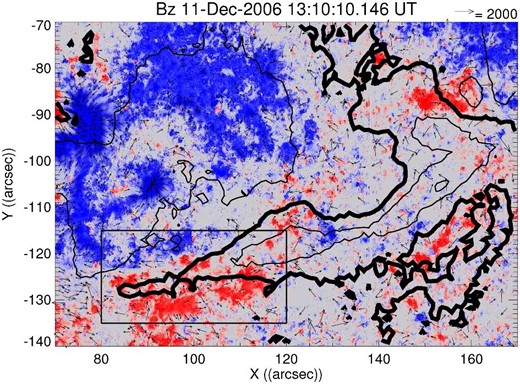
LOS (color) and transverse (arrows) components of the magnetic field obtained by the Milne–Eddington fitting procedure from the Hinode SOT/SP observations. The color plot is saturated at an absolute strength at 3 kG with dark blue (red) for negative (positive) field. Note that the orientation of the transverse components is determined by the component closest to the extracted potential field based on the observed LOS component distribution. Solid contours are for brightness in the Hα band taken at the Big Bear Solar Observatory. The thick contour line indicates the outline of the analyzed filament. The solid box indicates the region where the analysis was performed.
Figures 3a and 3c show the spatial distribution and histogram of the azimuth angle χB of the transverse component to the LOS of the magnetic field on 2006 December 11. χB is the anti-clockwise angle from the western direction (x direction). Note that only the data points with a strong polarization degree (>1%) are shown and that the values are 0 ≤ χB < 180° because the orientation of the transverse component is indistinguishable owing to the 180° ambiguity. The distribution peak is around χB ≈ 160°. The relative angle between this direction and the spine of the filament is χB − χf ≈ 150° or 30° in an acute angle, i.e., the field is strongly sheared (figure 4). This is consistent with the previous statistical results on the mid-latitude quiescent prominences by Leroy, Bommier, and Sahal-Brećhot (1984).
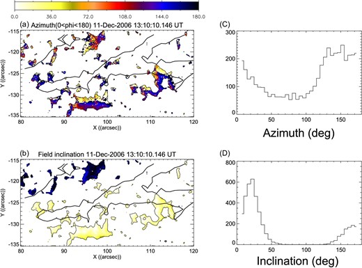
(a) Azimuth angle χB and (b) inclination γB of the magnetic field obtained by the Milne–Eddington fitting procedure from the Hinode SOT/SP observations on 2006 December 11. The azimuth is defined by the angle between the transverse component of the magnetic field and the heliocentric x-axis in the anti-clockwise direction. Because of the 180° ambiguity, the orientation of the transverse component is indistinguishable. The inclination is defined by the angle between the earthward direction and the magnetic field. The analyzed area is shown as a solid box in figure 2. Histograms are (c) the azimuth angle of the transverse components and (d) the inclination angle of the magnetic field. Note the strong peak in the bin for a value of zero include the data points of the weak polarization degree (<1%).
![Drawing showing the relative angle and location between the filament and the magnetic field. The dashed line indicates the location of the PIL which is along the filament with a χf ≈ 10° tilt from the east–west direction. The direction along the PIL in the solar surface is indicated by an element vector $\boldsymbol{e}_\parallel$ and the direction perpendicular to the PIL in the same plane by $\boldsymbol{e}_\perp$. The solid lines indicate the photospheric magnetic field with the azimuth angle χB obtained by SOT/SP. Note that the 180° ambiguity remains in the azimuth angle. The symbols “[+]” and “[−]” indicate the sign of the line-of-sight component of the magnetic field.](https://oup.silverchair-cdn.com/oup/backfile/Content_public/Journal/pasj/71/2/10.1093_pasj_psz014/3/m_pasj_71_2_46_f4.jpeg?Expires=1750467263&Signature=E0y-MBgm-A6X9XaUvjSQ8bF-qxUx9jA5qpIyV~oYcJg1j-9ISQnmrS5qDszUR3wJFDbkZmioxhMlhcC9BfiuQz2Ren12KU1W1W3JAaL2pKQ6iaITOB0octJWKnp6D7EznGwN7iQfzC87ccGYGzBu4sFq8LNopQcriKLgblW7Nj7c0YX7WAph6f2Fu2sHnt7x3plQdjC5uBVN-79Z7iWyUbQTYCUtMv6JkiG7wIHEhZ~GPcm9pWc7VDNH~COGmpjyyeTpcORu-tskWS-Y7DdUs89~y4EQ6Sm7CQbVMu4~tpG0yy4uABtqxd4hg4VzFi9FIV1ryhGf-CpQJEvMmem0Vw__&Key-Pair-Id=APKAIE5G5CRDK6RD3PGA)
Drawing showing the relative angle and location between the filament and the magnetic field. The dashed line indicates the location of the PIL which is along the filament with a χf ≈ 10° tilt from the east–west direction. The direction along the PIL in the solar surface is indicated by an element vector |$\boldsymbol{e}_\parallel$| and the direction perpendicular to the PIL in the same plane by |$\boldsymbol{e}_\perp$|. The solid lines indicate the photospheric magnetic field with the azimuth angle χB obtained by SOT/SP. Note that the 180° ambiguity remains in the azimuth angle. The symbols “[+]” and “[−]” indicate the sign of the line-of-sight component of the magnetic field.
Figures 5a–5d show the observation when this active region is near the east limb (Φ < 0). As noted in the beginning of this section, we regard the dark structures that appeared in these panels to be identical with those in figure 1 by comparing the continuous images (at least, one image per day) of the Hα observations. The LOS component B|$z$| of the photospheric field in the solid insets is found to be dominated by the positive (B|$z$| > 0, γB < 90°) below the filament in this location. On the other hand, it is negative (B|$z$| < 0, γB > 90°) when the filament is near the west limb (Φ > 0, figures 5e–5h). Thus, there is a variation of the sign in the LOS magnetic component B|$z$| consistent with the above formula (2), and one can also obtain the indication of B⊥ < 0. This means that the photospheric magnetic field below the filament has an inverse-polarity structure (see figure 4). Note that B∥ > 0, |$B_\Phi >0$|, and |$B_\Theta <0$| are also suggested from B⊥ < 0.
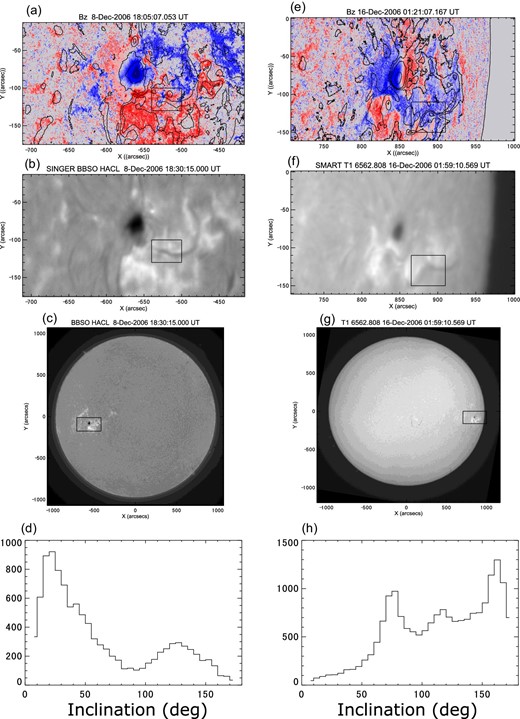
Observations of active region NOAA 10930 (a–d) near the eastern limb on 2006 December 8 and (e–h) near the western limb on 2006 December 16. Color maps in panels (a) and (e) show the line-of-sight component of the magnetic field derived by the Milne–Eddington fitting from the polarimetric observations by Hinode SOT/SP. The color plot is saturated at an absolute strength at 3 kG with dark blue (red) for negative (positive) field. The brightness distributions in the Hα band are shown as contours in panels (a) and (e), and as a gray-scale map in panels (b), (c), (f), and (g). The data from 2006 December 8 was taken at BBSO and that from 2006 December 16 by SMART at the Hida Observatory. Panels (d) and (h) show the histogram of the inclination angle of the magnetic field. The analyzed areas are shown as boxes in panels (a) and (e), respectively.
The photospheric magnetic field below the filament is indicated to have an inverse-polarity. This means that near the PIL, the magnetic fields have a bald-patch structure; that is, the field lines are in contact with the photospheric surface in a concave-up shape (Lites 2005). Although the global three-dimensional structure high up in the atmosphere is beyond the scope of this study, we have other supporting observational material for the flux rope interpretation of this filament. The Transition Region and Coronal Explorer (TRACE) EUV image in figure 6 shows bright features crossing above the filament in a southeast to northwest direction. This suggests that the overlying field is twisting the filament in a left-handed manner. This is consistent with the orientation of the transverse component of the photospheric field and the flux-rope interpretation.
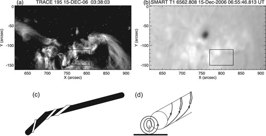
(a) TRACE 195 Å observations of active region NOAA 10930 at 3:38 UT on 2006 December 15. (b) The brightness distributions in the Hα band at 6:55 UT on the same date. The analyzed filament is shown by a solid line box. (c) Drawing to indicate the brightening above the dark filament in the TRACE image in panel (a). (d) A cartoon describing our explanation of the brightening feature.
The chirality (Martin 1998) of this filament is also investigated. Our results show that the axial spine field of the filament is in the westward direction. According to Martin’s definition, this filament has a dextral structure (see figure 10 of Martin 1998). The detailed structure of the filament material or the surrounding fibrils are not clear, owing to the insufficient spatial resolution of the available Hα images. The EUV image in figure 6a suggests that the coronal arcades are left-skewed, in a way that is consistent with the suggestions for the chirality made by Martin (1998). López Ariste et al. (2006) proposed a method to solve the 180° ambiguity in the azimuth angle of the magnetic field that uses the chirality of the filament. Our approach is different from theirs in that the chirality need not be known beforehand. It is obtained as a result of the solution of the ambiguity by using the information on the LOS component of the photospheric axial field when the filament is located near the limb.
The method of the current analysis includes several assumptions regarding the filament condition: There should be no drastic change in the filament magnetic field during the passage from the east to west limbs through the solar disk. If the filament is dynamic in nature, it is difficult to interpret the change of sign in the LOS component below the filament as a consequence of the viewpoint or change of structure. However, this method may add a new approach for studying a global magnetic structure of filaments. As long as stable polarimetric observational data are available, the orientation of the photospheric axial field can be obtained without high-resolution Hα data. This method may be especially promising for statistical studies.
4 Conclusions
This study focused on the Hinode observation of the photospheric magnetic structure below a filament and attempted to infer what magnetic structure the filament has in the equilibrium. We studied a filament in active region NOAA 10930 that appeared on the solar disk in 2006 December. The magnetic transverse component perpendicular to the LOS has a direction almost parallel to the filament spine with a shear angle of 30°, the orientation of which includes the 180° ambiguity. We used the center-to-limb variations for the solution of this ambiguity. When the filament is near the east limb, we found that the line-of-site magnetic component below the filament is positive, while it is negative near the west limb. This change of sign indicates that the horizontal photospheric field perpendicular to the polarity inversion line beneath the filament has an “inverse-polarity”, which indicates a flux-rope structure of the filament supporting field.
Acknowledgments
Hinode is a Japanese mission developed and launched by ISAS/JAXA, with NAOJ as domestic partner and NASA and STFC (UK) as international partners. It is operated by these agencies in co-operation with ESA and NSC (Norway). The Global High Resolution Hα Network is operated by the Big Bear Solar Observatory, New Jersey Institute of Technology in the USA. TRACE is a NASA Small Explorer mission. The authors are supported by JSPS KAKENHI Grant: T.Y. is by JP15H03640, M.S. by JP17K05397, Y. K. by JP18H05234 (PI: Y. K.) and JP25220703 (PI: S. Tsuneta), and JP15H05814 (PI: K. Ichimoto).
Appendix 1
Derivation of equations (2) and (3)
Appendix 2
MEKSY code
The fitting code MEKSY is developed by the authors of this paper. It is based on MELANIE (Socas-Navarro et al. 2008) for the fitting with the model atmosphere and PIKAIA (Charbonneau 2002)1 for the initial guess. The observed Stokes profiles are fitted by a spectral model to obtain the physical parameters in the solar photosphere. The model is based on the Milne–Eddington atmosphere in which the physical parameters, such as magnetic field strength, orientation, and Doppler velocity, are assumed to be homogeneous along the line of sight. An exact analytical solution is available as a set of explicit formulae known as the Unno–Rachkovsky solution. The details of this solution are described by, e.g., del Toro Iniesta (2003).
The fitting parameters are (1) magnetic field strength, (2) magnetic field inclination, (3) magnetic field azimuth, (4) line strength (the opacity ratio of the line to the continuum), (5) Doppler width, (6) ratio of the damping width and Doppler width, (7) Doppler velocity, (8) radiative source function, (9) gradient of the radiative source function, (10) macro-turbulence velocity, (11) stray-light fraction, and (12) wavelength shift of the stray-light component. The model profile is a blend of the polarized and the non-polarized components. The former is the radiation from the magnetized plasma in the solar atmosphere, and the latter is a mixture of the radiation from the non-magnetized plasma and that from the stray light in the instrument. The polarized component is synthesized based on the Unno–Rachkovsky formula using the above parameters, whereas the stray-light component is extracted as the average of the observed profiles over the pixels with a weak polarization degree in the corresponding scan map. The standard Levenberg–Marquardt (LM) method (e.g., Press et al. 1992) is used for the non-linear fitting algorithm. This part of MEKSY is a tuned-up version of MELANIE. Through the development of the code, we found that the quality of the convergence of the iterative procedures in the LM fitting is highly dependent on the initial-guess parameter sets. In MEKSY, they are provided by the PIKAIA code which is based on the genetic algorithm (Charbonneau 1995). For data input and output, the CFITSIO library (Pence 1999) is used.
The main purpose behind the development of the MEKSY code is the fulfilment of high-speed processing. One Hinode SP normal-mode map includes approximately a square of 1000 pixel points. This is an enormous number compared with the previous spectro-polarimetric data, e.g., the Advance Stokes Polarimeter typically has only 2562 pixel points. Hinode also observes the Sun with practically no interruption and may routinely produce large format data. The developed code is optimized as much as possible to meet these requirements. An IDL front-end macro program is also developed to submit parallel processes on the parallel computing system (grid engine system). As a result, the process time is 50 ms for each pixel by an Opteron 2.2 GHz core, and thus it takes 14 hours to build a ≈10002-pixel map. The process can be parallelized by using the parallel system so that the entire process takes less than an hour using a 16-CPU system. The code is installed on the grid engine system at the Hinode Science Center (HSC) in the National Astronomical Observatory of Japan.2 The program source is written in Fortran 90 and the technical details of the code including the user reference manual are available on the HSC website as online documents.3
Figure 7 shows the comparison of the fitting results with the existing code. We used the results of the so-called “ASP code” (Skumanich & Lites 1987; Lites et al. 1994) as a reference developed for the inversion of the Stokes data obtained by the Advanced Stokes Polarimeter (ASP). The results are almost consistent. Although there is crosstalk between the field strength and the stray-light fraction when the strength is weak, the average magnetic flux density is consistent (bottom panel of figure 7).
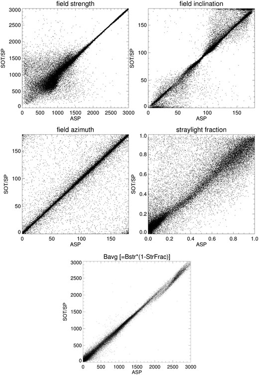
Scatter plots of the results for the different inversion codes. The vertical axis in each plot represents the results obtained by MEKSY, and the horizontal axis represents those obtained by the ASP code. Each point corresponds to each spatial pixel. Upper left: field strength in Gauss; upper right: field inclination in degrees; middle left: field azimuth in degrees; middle right: stray-light fraction (a complement of the filling factor); and bottom: magnetic flux density (i.e., the product of the filling factor and field strength).
Figure 8 shows the errors of the fitting as a function of the polarization degree in each spatial pixel. Note the data contains the image of the sunspot umbra where the Stokes profile has a complex figure, presumably because of the effect of the low-temperature molecular lines that are not taken into account in the present code. The branches extending in the relatively strong (≈0.1) polarization degree range are attributed to this effect. Otherwise, we may estimate the error of the fitting procedure using MEKSY. The 1σ errors in the pixels with polarization degrees greater than 2% are the following: a few gauss for field strength, a few degrees both for the field inclination and field azimuth, ≈10 m s−1 for the Doppler velocity, and ≈10% for the stray-light fraction. The error for each variable is calculated as δak = (χ2/αkk)1/2, where ak (k = 1, ..., 12) is the fitting parameter given above and δak is its fitting error, χ2 is the value of the merit function for the obtained fit results, and αkk is the kth diagonal component of the “curvature matrix”, defined as the curvature of the merit function χ2(ak) in the fitting parameter space. The detailed definitions of these variables are given in Press et al. (1992).
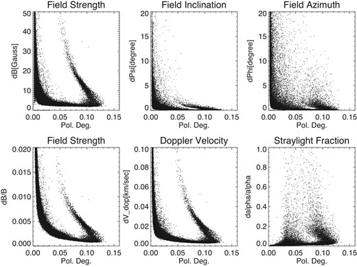
Derivation errors as functions of the polarization degrees in each pixel. Top left: field strength in Gauss; top center: field inclination in degrees; top right: field azimuth in degrees; bottom left: the ratio of the error in field strength to the amount; bottom center: Doppler velocity; and bottom right: the ratio of the error in the stray-light fraction to the amount.
Footnotes
Charbonneau, P. 2002, NCAR Technical Note NCAR/TN-450+IA 〈https://www.hao.ucar.edu/modeling/pikaia/pikaia.php〉.
The system started its operation in 2006 and was shut down in February 2013. A similar system is in operation as part of the multi-wavelength data analysis system of the Astronomy Data Center, NAOJ.
References
