An image reconstruction method for an X-ray telescope system with an angular resolution booster

Morii, Mikio; Ikeda, Shiro; Maeda, Yoshitomo

doi:10.1093/pasj/psy143

Abstract

We propose an image reconstruction method for an X-ray telescope system with an angular resolution booster proposed by Maeda et al. (2018, PASJ, submitted). The system consists of double multi-grid masks in front of an X-ray mirror and an off-focused two-dimensional imager. Because the obtained image is off-focused, an additional image reconstruction process is assumed to be included. Our image reconstruction method is an extension of the traditional Richardson–Lucy algorithm with two regularization terms, one for sparseness and the other for smoothness. Such a combination is desirable for astronomical imaging because astronomical objects have a variety in shape, from point sources to diffuse sources to mixtures of both. The performance of the system is demonstrated with simulated data for point sources and diffuse X-ray sources such as Cas A and the Crab Nebula. The image resolution is improved from a few arcmin of focused image without the booster to a few arcsec with the booster. Through the demonstration, the angular resolution booster with the image reconstruction method is shown to be feasible.

1 Introduction

Among X-ray telescopes, the Chandra X-ray satellite (Weisskopf et al. 2000) attains the best angular resolution (⁠|${0{^{\prime \prime}_{.}}5}$|⁠). However, the effective area of the focusing mirror is not large enough to collect photons for statistical study of time variation and energy spectrum. X-ray telescopes like Suzaku (Mitsuda et al. 2007) and Hitomi (Takahashi et al. 2016) were designed to have moderately high angular resolution of a few arcmin and a large effective area. If the angular resolution of the Suzaku/Hitomi telescopes had been improved to a few arcsec while preserving the effective area, different scientific topics would have been revealed. Two examples are described below.

The first example is the lensed quasar. Chartas et al. (2017) and references therein monitored several lensed quasars at multiple wavelengths, including Chandra X-ray measurements. They found red-shifted and blue-shifted Fe Kα lines in the spectra of lensed images. They interpreted the shift of the Fe Kα line as resulting from gravitational and special relativistic Doppler effects. Since the image separation of lensed quasars is generally larger than a few tenths of arcsec, often down to a few arcsecs, the larger effective area with an angular resolution of arcsecs becomes a unique probe of lensed quasars. The other example is the study of supernova remnants. Uchiyama and Aharonian (2008) and Sato et al. (2018) revealed the mechanism of particle acceleration in supernova remnants by observing the time variation of the shell in arcsec resolution for the bright supernova remnant Cas A (Hughes et al. 2000) with Chandra. More such studies are desired using telescopes with larger effective areas than Chandra.

Recently, our companion paper (Maeda et al. 2018) has proposed a simple angular resolution booster for an X-ray telescope like Hitomi, which can possibly improve the angular resolution by an order of 1–2, at low cost. The system consists of a set of multi-grid masks in front of the X-ray mirror and a two-dimensional imager at a position slightly off-focused from the focal plane. The idea is to utilize the shadow pattern shed on the imager through the masks which contains information at a higher angular resolution than that obtained only with the mirror. Since the imager’s position is off-focused, the system needs to reconstruct the sky image from the observed pattern.

For the image reconstruction, the Richardson–Lucy algorithm (Richardson 1972; Lucy 1974) is well known as a method to obtain the sky image from data following Poisson statistics. Ikeda et al. (2014) modified the method with a sparseness regularizer. In this paper, we show a new image reconstruction method by extending these methods with two regularization terms, where one is for sparseness and the other is for smoothness.

Starck, Pantin, and Murtagh (2002) and Puetter, Gosnell, and Yahil (2005) reviewed image deconvolution methods using Fourier or wavelet bases for improvement of image resolution, which take a different approach from our work.

2 Mathematical formulation of the problem

In this article, the image is an M = m × n-pixel rectangular region. This corresponds to a rectangular area on the tangential plane of the celestial sphere. Each pixel is indexed with u = (i, j) (i = 1, …, m; j = 1, …, n). The astronomical image is expressed by the distribution of photon intensity per unit dimension (for example, per unit sky area per unit time, deg⁻² s⁻¹, or per unit sky area per unit time per unit energy range, deg⁻² s⁻¹ erg⁻¹, etc.). Here, we express the astronomical image I(u) at each pixel u as a non-negative real value. On the other hand, pixels of an off-focus plane detector are indexed with |$v$| (⁠|$v$| = 1, …, V). The number of photons in an exposure (an observation) of the telescope detected at pixel |$v$| is Y(⁠|$v$|⁠), which is a non-negative integer value. It follows a Poisson distribution, Y(⁠|$v$|⁠) ∼ Poisson[∑_ut(⁠|$v$|⁠, u)I(u)], where t(⁠|$v$|⁠, u) is the response of the detector (including the telescope and imager responses) from a pixel u with unit intensity. We assume that each element of the response matrix is a non-negative value normalized by ∑_|$v$|t(⁠|$v$|⁠, u) = 1. The normalized image ρ(u) is expressed by |$\rho (u) = \frac{I(u)}{S}$|⁠, where S = ∑_uI(u).

The joint distribution of Y_|$v$| is described as a product of two probability functions. One is the distribution of ∑_|$v$|Y_|$v$|, which follows the Poisson distribution Poisson(∑_|$v$|Y_|$v$|; S), and the other is that of Y_|$v$|, which follows the multinomial distribution Multinomial[{Y_|$v$|}; {∑_ut(⁠|$v$|⁠, u)ρ_u}]:

\begin{eqnarray} P(Y | I) & = & \prod _v {\rm Poisson} \left[ Y_v ; \sum _u t(v, u) I(u) \right] \nonumber \\ & = & \frac{e^{-S} S^{(\sum _v Y_v)}}{(\sum _v Y_v)!} \times \frac{(\sum _v Y_v)!}{\prod _v Y_v!} \prod _v \left[ \sum _u t(v, u) \rho _u \right]^{Y_v} \nonumber \\ & = & {\rm Poisson} \left(\sum _v Y_v ; S \right) \nonumber\\ && \times\, {\rm Multinomial} \left[\lbrace Y_v\rbrace ; \Bigl \lbrace \sum _u t(v, u) \rho _u \Bigr \rbrace \right]. \end{eqnarray}

(1)

The above equation shows that S and ρ can be estimated separately. A natural estimate of S is the maximum likelihood estimator, which is easily obtained as S* = ∑_|$v$|Y(⁠|$v$|⁠). So, from now on, we consider only the likelihood function of ρ. By taking the logarithm and neglecting the terms independent of ρ, the likelihood function for ρ becomes L_ρ(ρ) = ∑_|$v$|Y(⁠|$v$|⁠)log [∑_ut(⁠|$v$|⁠, u)ρ(u)].

It is known that the maximum likelihood of L_ρ(ρ) is calculated by the Richardson–Lucy algorithm (Richardson 1972; Lucy 1974). However, when the number of the photons is small, the estimated image becomes unstable. This is because the information required to reconstruct the m × n image is much larger compared to the limited photon counts.

In order to overcome the problem, we propose a method based on sparse modeling. Sparse modeling is a new signal processing method. Assuming sparseness of the image in some domain, the amount of information to be estimated is reduced. In this case, we assume the image ρ is sparse (many pixels are zeros) and smooth. Under this assumption, the image would be reconstructed from limited photons. These two assumptions are suitable for astronomical imaging, because astronomical objects have a variety of shapes, from point sources to diffuse sources (e.g., supernova remnants, clusters of galaxies, pulsar wind nebulae) to mixtures of them (e.g., point sources in Galactic planes).

A common implementation of the sparse modeling is to use additional regularization terms for the optimization. In our case, we employ a term to encourage the sparseness and another term for smoothness. A widely used regularization term for sparseness is the ℓ₁ norm, but it does not work in this case since ‖ρ(u)‖₁ = ∑_uρ(u) = 1 from its definition. Thus, we follow the idea in Ikeda et al. (2014), which uses the following term:

\begin{equation} (1-\beta ) \sum _u\log \rho (u), 0< \beta . \end{equation}

(2)

Here, the parameter β( > 0) controls the sparseness. Smaller β produces a sparser image, and the term disappears when β = 1. We call this the Dirichlet term, since it is related to the Dirichlet distribution.

For the regularization of smoothness, we add the following regularization term in the log-likelihood, which works to decrease the difference in pixel values between adjoining pixels:

\begin{eqnarray} V({\rho }) & = & \sum _{i = 1}^{m - 1} \sum _{j = 1}^{n - 1} \left[ (\rho _{i,j} - \rho _{i + 1,j})^2 + (\rho _{i,j} - \rho _{i,j + 1})^2 \right] \nonumber \\ & & +\, \sum _{i = 1}^{m - 1} (\rho _{i,n} - \rho _{i + 1,n})^2 + \sum _{j = 1}^{n - 1} (\rho _{m,j} - \rho _{m, j+1})^2 . \end{eqnarray}

(3)

Finally, the cost function of ρ to be minimized becomes

\begin{equation} L(\rho ) = - L_\rho (\rho ) + (1 - \beta ) \sum _u \log \rho (u) + \mu V(\rho ), \nonumber \end{equation}

(4)

where the hyperparameters β and μ control the degree of sparseness and smoothness, respectively. We optimize ρ in the valid region for sky images: C = {ρ ∈ R^M∣ρ_u ≥ 0, ∑_uρ_u = 1}.

The optimization problem of maximizing L_ρ(ρ) is known to be solved by the Richardson–Lucy algorithm (Richardson 1972; Lucy 1974), which is indeed the expectation–maximization (EM) algorithm for a distribution obeying Poisson statistics (Dempster et al. 1977). The problem of maximizing L_ρ(ρ) − (1 − β)∑_ulog ρ(u) is also solved with the EM algorithm, as shown in Ikeda et al. (2014). The current problem cannot be solved only with the EM algorithm, so we have combined the EM algorithm and the proximal gradient method in order to solve it (e.g., Beck & Teboulle 2009).

3 Algorithm for the reconstruction

At first, we apply the EM algorithm for the optimization of the cost function; then the rth step in the EM M-step becomes

\begin{eqnarray} \rho ^{(r + 1)} & = & \mathop {\rm arg~min}\limits _{\rho \in C} \Big[ L_{\rm sub} \equiv - \sum _u m_u^{(r)} \log \rho _u + (1 - \beta ) \nonumber\\ && \times\, \sum _u \log \rho _u + \mu V(\rho ) \Big], \end{eqnarray}

(5)

where

\begin{equation} m_u^{(r)} = \sum _{v} Y(v) \frac{ t(v, u) \rho _u^{(r)}}{ \sum _{u} t(v, u) \rho _u^{(r)} } \quad (r = 1, 2, \ldots ). \end{equation}

(6)

To solve the sub-problem, we use the proximal gradient method as shown in Beck and Teboulle (2009). Here, we divide L_sub into two terms, L_sub = g(ρ) + f(ρ), where f(ρ) = μV(ρ) and |$g(\rho ) = - \sum _u [m_u^{(r)} - (1 - \beta )] \log \rho _u$|⁠. We follow the algorithm of “ISTA with backtracking.” Then the updating rule of the proximal gradient method in the kth step becomes

\begin{eqnarray} \rho ^{(k + 1)} & = & \mathop {\rm {arg\, min}}\limits _{\rho \in C} \sum _u \Bigg[ \frac{L_k}{2} \big(\rho _u - \sigma _u^{(k)}\big)^2 \nonumber\\ && -\, [m_u^{(r)} -\, (1 - \beta )] \log \rho _u \Bigg], \end{eqnarray}

(7)

where

\begin{equation} \sigma _u^{(k)} = \rho _u^{(k)} - \frac{\mu }{L_k} \frac{\partial V(\rho ^{(k)})}{\partial \rho _u} \quad (k = 1, 2, \ldots ). \end{equation}

(8)

Here, the Lipschitz constant L_k is searched for in each k-step. This minimization problem can be solved in a closed form by introducing a Lagrange multiplier— the details are shown in the Appendix. Then, we can solve this minimization problem for a fixed (β, μ). Since the reconstructed image depends on the hyperparameters (β, μ), we determine the best parameters by cross-validation.

4 Results

We test the performance of our proposed reconstruction method by using simulated observed images. To make the simulated images and perform the image reconstruction, we use the response of the detector t(⁠|$v$|⁠, u). This is made by the ray-tracing code “xrtraytrace” (T. Yaqoob et al. in preparation). The optics parameter of a Hitomi SXT-like lightweight telescope (Okajima et al. 2016) is adopted in the ray-tracing. The angular resolution we set for this ray-tracing is about 1″. The off-focus images through the double masks are calculated by offsets with a 2″ pitch. See Maeda et al. (2018) for the details.

We simulate images of double point sources with a close separation of 4″ and diffuse sources such as Cas A and Crab Nebula. The input images are shown in figures 1a, 1e, and 1i, and the simulated observed images on the off-focus imager are figures 1b, 1f, and 1j. The image sizes of both the off-focus imager and the reconstructed sky image are 60 × 60 pixels. We implemented the algorithm in C++, utilizing the BLAS library.²

Fig. 1.

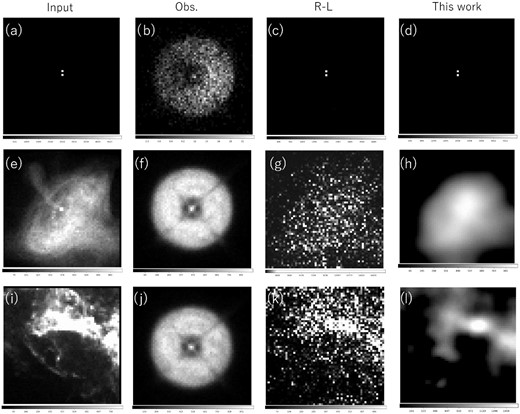
Image reconstruction for double stars (top), Crab nebula (middle), and Cas A (bottom). The input images are shown in the first column. Panel (a) is double stars with a separation of 4″. Panels (e) and (i) are images of the Crab Nebula and Cas A obtained with the Chandra X-ray satellite,¹ respectively. The second columns are simulated observed images on the off-focus imager. The number of photons from the two stars is 5 × 10³ photons each (b), and the total number of photons for the Crab Nebula and Cas A are 10⁶ (f) and (j). The reconstructed images by the Richardson–Lucy method and our proposed method are shown in the third and fourth columns, respectively. Panels (d), (h), and (l) are the results with the best hyperparameters, (β, log₁₀μ) = (0.6, 1.0), (0.6, 8.0), and (0.9, 7.0), respectively. The pixel scales of the input and reconstructed images are 2″ per pixel. The images here and elsewhere are made in the look-down geometry.

Open in new tab Download slide

Figures 2 and 3 show the reconstructed images of the double point sources and Cas A along with the hyperparameters varied. The best reconstructed image with the best hyperparameters is determined by ten-fold cross-validation and shown as the marked panel in these figures. Here, we search among 121 pairs of (β, μ): β is varied from 0.1 to 1.1 in steps of 0.1, and log₁₀μ is varied from 0 to 10 in steps of 1. The right two columns of figure 1 present the reconstructed images for the double stars, the Crab Nebula and Cas A, obtained by the Richardson–Lucy method and our proposed method.

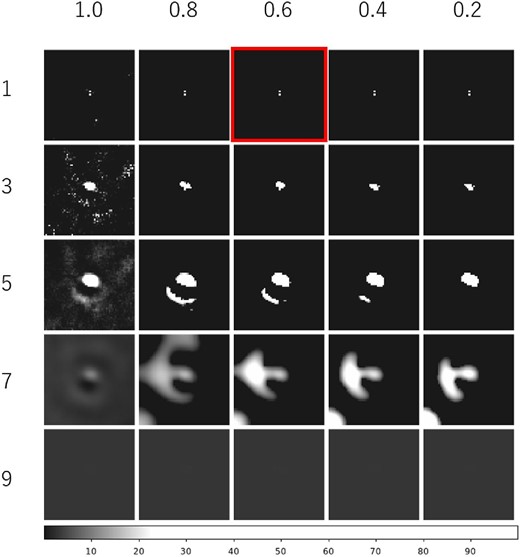
Reconstructed double star images by changing the hyperparameters (β, log10μ). The sparsity and smoothness increase from left to right and from top to bottom, by setting β and log10μ as shown above and to the left of the figure, respectively. The best image determined by the cross-validation is marked with a red frame. (Color online)

Fig. 2.

Reconstructed double star images by changing the hyperparameters (β, log₁₀μ). The sparsity and smoothness increase from left to right and from top to bottom, by setting β and log₁₀μ as shown above and to the left of the figure, respectively. The best image determined by the cross-validation is marked with a red frame. (Color online)

Open in new tab Download slide

Fig. 3.

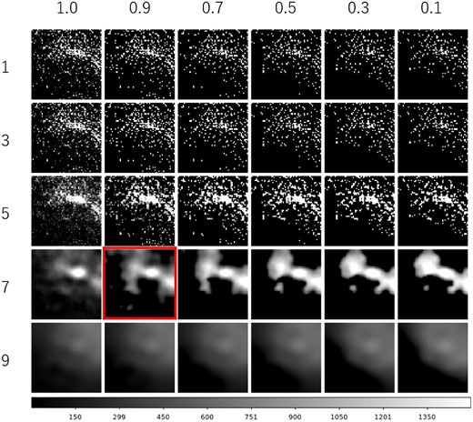
As figure 2, but for Cas A. (Color online)

Open in new tab Download slide

To estimate the angular resolution of our method, we evaluate the successful separation rate for two close point sources with an angular distance of 4″ as shown in figure 1a for 100 simulations. In the cases of 10⁴, 10³, and 10² total photons, the success rates are 100% (100 out of 100 trials), 99% (99/100), and 12% (12/100), respectively.

The processing speed is measured by using a budget computer equipped with a 3.20 GHz Intel Core i7 processor: an image with 60 × 60 pixels is reconstructed in 70 s on average for each hyperparameter.

5 Discussion and conclusion

In reconstructing double stars with close separation (figure 1d), we demonstrated that the booster system with our image reconstruction method can achieve a superb resolution of 4″ if the photon count from a point source is more than about 5 × 10².

Although the reconstructed images vary with the parameters (β, μ) as shown in figures 2 and 3, the best parameters can be determined by cross-validation, and the best image looks plausible. For point sources, a small smoothness parameter is selected by the cross-validation (figure 2), while for diffuse objects, large smoothness parameters are selected. As shown in figure 1, the images obtained by the Richardson–Lucy method are noisy, while the images obtained by our method are less noisy and look similar to the input images.

As shown in the second paragraph of section 2, the total intensity of the X-ray image and the pattern of the image are estimated separately. Then, the total intensity is simply estimated by S*, and the 1 σ error by the square root of S*. The reconstructed pattern of images depends on the balance between the photon statistics and the complexity of the input images. Roughly speaking, complex images require larger photon statistics than images containing sparse point sources. Quantitative estimation of the necessary number of photons for the reconstruction will be undertaken in future work. In this paper, the energy dependency of an X-ray image is not taken into consideration. Reconstruction of both image and energy spectrum at once would be the next challenge, e.g., by introducing regularization of the smoothness for the energy channel.

In this paper, we have successfully demonstrated that 1–2 orders of magnitude improvement of angular resolution can be realized by using an angular resolution booster combined with image reconstruction. This system needs only a simple, thus possibly low-cost, modification to the current well-established telescopes. Thus, our method will progress X-ray astronomy in the near future.

Acknowledgements

This research is supported by CREST, the Japan Science and Technology Agency (JST), JPMJCR1414, and in part by JSPS Grant-in-Aid for Scientific Research (KAKENHI) Grant No. 17K05395. YM gratefully acknowledges funding from the Tanaka Kikinzoku Memorial Foundation.

Appendix.

Solution of the sub-problem

An iteration step of optimization in the proximal gradient method, equation (7), is solved by minimizing the following Lagrangian with a Lagrange multiplier τ:

\begin{eqnarray} l(\rho , \tau ) & = & \sum _u \left\lbrace - [m_u^{(r)} - (1 - \beta )] \log \rho (u) + \frac{L_k}{2} \left(\rho _u - \sigma _u^{(k)} \right)^2 \right\rbrace \nonumber\\ && +\, \tau \left( \sum _u \rho _u- 1 \right). \end{eqnarray}

(A1)

By fixing τ, it is solved in a closed form:

\begin{equation} \rho _u(\tau ) = \left\lbrace \begin{array}{ll}\frac{1}{2} \left[ b_u^{(k)}(\tau ) + \sqrt{ D_u^{(k)}(\tau ) } \right] , [m_u^{(r)} \!-\! (1 \!-\! \beta ) > 0] , \\ b_u^{(k)}(\tau ) & [m_u^{(r)} \!-\! (1 \!-\! \beta ) = 0] , \\ 0 & [m_u^{(r)} \!-\! (1 \!-\! \beta ) < 0] , \end{array} \right. \end{equation}

(A2)

where

\begin{eqnarray} D_u^{(k)}(\tau ) = {b_u^{(k)}(\tau )}^2 + 4 \frac{m_u^{(r)} - (1 - \beta )}{L_k}, \end{eqnarray}

(A3)

\begin{eqnarray} b_u^{(k)}(\tau ) = \sigma _u^{(k)} - \frac{\tau }{L_k}. \end{eqnarray}

(A4)

Here, τ must satisfy the condition s(τ) = ∑_uρ_u(τ) − 1 = 0. Since the function s(τ) is convex, the solution can be obtained by the Newton–Raphson method. The updating rule of the ith Newton–Raphson step is

\begin{equation} \tau ^{(i + 1)} = \tau ^{(i)} - \frac{s(\tau ^{(i)})}{s^\prime (\tau ^{(i)})}, \end{equation}

(A5)

where

\begin{eqnarray} s^\prime (\tau ) = \sum _u \rho _u^\prime (\tau ), \end{eqnarray}

(A6)

\begin{eqnarray} \rho _u^\prime (\tau ) & = & \left\lbrace \begin{array}{ll}- \frac{1}{2 L_k} \frac{ b_u^{(k)}(\tau ) + \sqrt{ D_u^{(k)}(\tau ) } }{\sqrt{ D_u^{(k)}(\tau ) }} & [m_u^{(r)} - (1 - \beta ) > 0] , \\ -\frac{1}{L_k} & [m_u^{(r)} - (1 - \beta ) = 0] , \\ 0 & [m_u^{(r)} - (1 - \beta ) < 0] . \end{array} \right. \end{eqnarray}

(A7)

Footnotes

1

NASA HEASARC 〈https://heasarc.gsfc.nasa.gov/〉.

2

〈http://www.netlib.org/blas/〉.

References

Beck

A.

,

Teboulle

M.

2000

,

SIAM J. Imaging Sci

.,

2

,

183

Crossref

Search ADS

Chartas

G.

,

Krawczynski

H.

,

Zalesky

L.

,

Kochanek

C. S.

,

Dai

X.

,

Morgan

C. W.

,

Mosquera

A.

2017

,

ApJ

,

837

,

26

Crossref

Search ADS

Dempster

A. P.

,

Laird

N. M.

,

Rubin

D. B. J. R.

1977

,

Statistical Soc. Ser. B

,

39

,

1

Hughes

J. P.

,

Rakowski

C. E.

,

Burrows

D. N.

,

Slane

P. O.

2000

,

ApJ

,

528

,

L109

Crossref

Search ADS

Ikeda

S.

,

Odaka

H.

,

Uemura

M.

,

Takahashi

T.

,

Watanabe

S.

,

Takeda

S.

2014

,

Nucl. Inst. Meth. Phys. Res. A

,

760

,

46

Crossref

Search ADS

Lucy

L. B.

1974

,

AJ

,

79

,

745

Crossref

Search ADS

Maeda

Y.

,

Iizuka

R.

,

Hayashi

T.

,

Ishida

M.

,

Sato

T.

,

Ikeda

S.

,

Morii

M.

2018

,

PASJ

,

submitted

Mitsuda

K.

et al.

2007

,

PASJ

,

59

,

S1

Crossref

Search ADS

Okajima

T.

et al.

2016

,

SPIE Proc

.,

9905

,

99050Z

Puetter

R. C.

,

Gosnell

T. R.

,

Yahil

A.

2005

,

ARA&A

,

43

,

139

Crossref

Search ADS

Richardson

W. H.

1972

,

J. Opt. Soc. Am

.,

62

,

55

Crossref

Search ADS

Sato

T.

,

Katsuda

S.

,

Morii

M.

,

Bamba

A.

,

Hughes

J. P.

,

Maeda

Y.

,

Ishida

M.

,

Fraschetti

F.

2018

,

ApJ

,

853

,

46

Crossref

Search ADS

Starck

J. L.

,

Pantin

E.

,

Murtagh

F.

2002

,

PASP

,

114

,

1051

Crossref

Search ADS

Takahashi

T.

et al.

2016

,

Proc. SPIE

,

9905

,

99050U

Uchiyama

Y.

,

Aharonian

F. A.

2008

,

ApJ

,

677

,

L105

Crossref

Search ADS

Weisskopf

M. C.

,

Tananbaum

H. D.

,

Van Speybroeck

L. P.

,

O’Dell

S. L.

2000

,

SPIE Proc

.,

4012

,

2

Crossref

Search ADS

This article is published and distributed under the terms of the Oxford University Press, Standard Journals Publication Model (https://dbpia.nl.go.kr/journals/pages/open_access/funder_policies/chorus/standard_publication_model)

Download all slides

Month:	Total Views:
January 2019	21
February 2019	22
March 2019	8
April 2019	16
May 2019	5
June 2019	6
July 2019	11
August 2019	4
September 2019	9
October 2019	6
November 2019	2
December 2019	2
January 2020	2
March 2020	1
April 2020	6
June 2020	3
November 2020	3
January 2021	5
February 2021	3
March 2021	11
April 2021	5
May 2021	4
June 2021	7
July 2021	5
August 2021	6
September 2021	6
October 2021	2
November 2021	6
December 2021	13
January 2022	7
March 2022	2
April 2022	4
May 2022	4
June 2022	6
July 2022	12
August 2022	15
September 2022	10
October 2022	2
November 2022	9
December 2022	11
January 2023	12
February 2023	9
March 2023	6
April 2023	7
May 2023	4
June 2023	6
July 2023	6
August 2023	5
September 2023	12
October 2023	5
November 2023	6
December 2023	14
January 2024	6
February 2024	16
March 2024	8
April 2024	10
May 2024	10
June 2024	10
July 2024	11
August 2024	8
September 2024	14
October 2024	3
November 2024	8
December 2024	8
January 2025	8
February 2025	9
March 2025	6
April 2025	13
May 2025	3

Article Contents

An image reconstruction method for an X-ray telescope system with an angular resolution booster

Abstract

1 Introduction

2 Mathematical formulation of the problem

3 Algorithm for the reconstruction

4 Results

5 Discussion and conclusion

Acknowledgements

Appendix.

Solution of the sub-problem

Footnotes

References

Citations

Views

Altmetric

Email alerts

Astrophysics Data System

Citing articles via

Latest

Most Read

Most Cited

Article Contents

An image reconstruction method for an X-ray telescope system with an angular resolution booster Free

Abstract

1 Introduction

2 Mathematical formulation of the problem

3 Algorithm for the reconstruction

4 Results

5 Discussion and conclusion

Acknowledgements

Appendix.

Solution of the sub-problem

Footnotes

References

Citations

Views

Altmetric

Email alerts

Astrophysics Data System

Citing articles via

Latest

Most Read

Most Cited

This Feature Is Available To Subscribers Only

An image reconstruction method for an X-ray telescope system with an angular resolution booster