Hermite integrator for high-order mesh-free schemes

Yamamoto, Satoko; Makino, Junichiro

doi:10.1093/pasj/psy137

Abstract

In most mesh-free methods, the calculation of interactions between sample points or “particles” is the most time-consuming. When we use mesh-free methods with high spatial orders, the order of the time integration should also be high. If we use usual Runge–Kutta schemes, we need to perform the interaction calculation multiple times per time step. One way to reduce the number of interaction calculations is to use Hermite schemes, which use the time derivatives of the right-hand side of differential equations, since Hermite schemes require a smaller number of interaction calculations than Runge–Kutta schemes do to achieve the same order. In this paper, we construct a Hermite scheme for a mesh-free method with high spatial orders. We performed several numerical tests with fourth-order Hermite schemes and Runge–Kutta schemes. We found that, for both Hermite and Runge–Kutta schemes, the overall error is determined by the error of spatial derivatives, for time steps smaller than the stability limit. The calculation cost at the time-step size of the stability limit is smaller for Hermite schemes. Therefore, we conclude that Hermite schemes are more efficient than Runge–Kutta schemes and thus useful for high-order mesh-free methods for Lagrangian hydrodynamics.

1 Introduction

Lagrangian mesh-free methods, in which particles move following the motion of fluid, have been widely used for astrophysical hydrodynamical simulations. In most mesh-free methods, the calculation of interactions between particles is the most time-consuming part. Typically, one particle interacts with ∼ 100 neighbor particles, and thus the cost of interaction calculations dominates the total calculation cost. One way to reduce the number of interaction calculations is to use Hermite schemes, which use the time derivatives of the right-hand side of differential equations, since Hermite schemes require a smaller number of interaction calculations than Runge–Kutta schemes do to achieve the same order.

In the field of stellar dynamics, the fourth-order Hermite scheme (Makino 1991; Makino & Aarseth 1992) is widely used for high-order integration. The basic idea of the Hermite scheme is to calculate the time derivative of gravitational acceleration directly, and use it to construct a high-order interpolation polynomial. If we calculate up to a pth-order time-derivative directly, we can achieve the order of s(p + 1) when we use the s-step linear multi-step method, and in the case of s = 2, we can achieve the order of 2(p + 1). The two-step linear multi-step method can be formulated so that it requires only one force evaluation per time step. In the case of a grid-based scheme for hydrodynamics, Aoki (1997) described a method based purely on the Taylor expansion, which achieves the order p + 1.

In this paper, we combine the Hermite scheme with Consistent Particle Hydrodynamics in Strong Form (CPHSF: Yamamoto & Makino 2017), which is one of the high-order mesh-free methods. One disadvantage of the Hermite scheme is that, even though it requires a smaller number of interaction calculations, the calculation cost of one interaction is higher because we need to calculate high-order derivations. In the case of CPHSF or other moving least squares-based interpolation, high-order interpolation polynomial gives spatial derivatives, and we only need to convert spatial derivatives to time derivations using the original differential equations. Thus, the increase of the calculation cost is small and independent of the number of neighbors.

We performed several numerical tests. Fourth-order Hermite schemes and second- and fourth-order Runge–Kutta schemes are used for the test with a periodic boundary, and an implicit Hermite scheme, an implicit fourth-order Runge–Kutta scheme and the backward-Euler scheme are used for the test with boundary conditions. We found that, for both the Hermite and Runge–Kutta schemes, the overall error is determined by the error of spatial derivatives, for time steps smaller than the stability limit. The calculation cost at the time-step size of the stability limit is smaller for Hermite schemes. Therefore, we conclude that Hermite schemes are more efficient than Runge–Kutta schemes and thus useful for high-order mesh-free methods for Lagrangian hydrodynamics.

In the rest of this paper, we first present the formulation of the Hermite scheme for CPHSF in section 2, and report the results of numerical tests in section 3. We summarize our study in section 4.

2 Derivation of the high-order scheme

In this section, we present the derivation of the fourth-order Hermite schemes for CPHSF.

2.1 Hermite scheme

In this section we present the formulation of the fourth-order Hermite schemes (Makino 1991; Makino & Aarseth 1992). Consider a second-order differential equation,

\begin{eqnarray} \frac{d\boldsymbol{x}}{dt} &=& \boldsymbol{v}, \end{eqnarray}

(1)

\begin{eqnarray} \frac{d\boldsymbol{v}}{dt} &=& \boldsymbol{a}(\boldsymbol{x}). \end{eqnarray}

(2)

Here, |$\boldsymbol{x}$| and |$\boldsymbol{v}$| denote the position and velocity of one particle. The fourth-order Hermite scheme is derived as follows. The predictor at time t_n is given by

\begin{eqnarray} \boldsymbol{x}_{p} &=& \boldsymbol{x}_n + \boldsymbol{v}_n \Delta t + \frac{\boldsymbol{a}_n}{2} \Delta t^2 + \frac{\boldsymbol{j}_n}{6} \Delta t^3, \end{eqnarray}

(3)

\begin{eqnarray} \boldsymbol{v}_{p} &=& \boldsymbol{v}_n + \boldsymbol{a}_n \Delta t + \frac{\boldsymbol{j}_n}{2} \Delta t^2, \end{eqnarray}

(4)

where |$\boldsymbol{x}_{p}$| and |$\boldsymbol{v}_{p}$| are the predicted position and velocity at the new time, t_{n + 1} = t_n + Δt, |$\boldsymbol{x}_n$| and |$\boldsymbol{v}_n$| are the position and velocity at time t_n, and |$\boldsymbol{a}_n$| and |$\boldsymbol{j}_n$| are the acceleration and jerk (first time-derivative of acceleration) at time t_n. Using |$\boldsymbol{x}_{p}$| and |$\boldsymbol{v}_{p}$|⁠, we can now calculate the acceleration and jerk, |$\boldsymbol{a}_{n+1}$| and |$\boldsymbol{j}_{n+1}$|⁠, at time t_{n + 1}. Using |$\boldsymbol{a}_n$|⁠, |$\boldsymbol{j}_n$|⁠, |$\boldsymbol{a}_{n+1}$|⁠, and |$\boldsymbol{j}_{n+1}$|⁠, we can construct the third-order Hermite interpolation polynomial for |$\boldsymbol{a}(t)$| as

\begin{eqnarray} \boldsymbol{a}(t) &=& \boldsymbol{a}_n + \boldsymbol{j}_n (t - t_n) + \frac{\boldsymbol{s}_n}{2}(t-t_n)^2 + \frac{\boldsymbol{c}_n}{6}(t-t_n)^3, \end{eqnarray}

(5)

where |$\boldsymbol{s}_n$| and |$\boldsymbol{c}_n$| are given by

\begin{eqnarray} \boldsymbol{s}_n &=& \frac{-6(\boldsymbol{a}_n - \boldsymbol{a}_{n+1}) - \Delta t(4\boldsymbol{j}_n + 2\boldsymbol{j}_{n+1})}{\Delta t^2}, \end{eqnarray}

(6)

\begin{eqnarray} \boldsymbol{c}_n &=& \frac{12(\boldsymbol{a}_n - \boldsymbol{a}_{n+1}) + 6\Delta t(\boldsymbol{j}_n + \boldsymbol{j}_{n+1})}{\Delta t^3}. \end{eqnarray}

(7)

We integrate equation (5) from t_n to t_{n + 1} and obtain correctors given by

\begin{eqnarray} \boldsymbol{x}_c &=& \boldsymbol{x}_{p} + \frac{\boldsymbol{s}_n}{24} \Delta t^4 + \frac{\boldsymbol{c}_n}{120} \Delta t^5, \end{eqnarray}

(8)

\begin{eqnarray} \boldsymbol{v}_c &=& \boldsymbol{v}_{p} + \frac{\boldsymbol{s}_n}{6} \Delta t^3 + \frac{\boldsymbol{c}_n}{24} \Delta t^4. \end{eqnarray}

(9)

If we set |$\boldsymbol{x}_{n+1} = \boldsymbol{x}_c$| and |$\boldsymbol{v}_{n+1} = \boldsymbol{v}_c$| at this point, that means we use the PEC (predict–evaluate–correct) form of the linear multi-step method. We can also use PECE or P(EC)² forms.

2.2 Derivation of high-order time-derivatives for hydrodynamical equations

In this section, we describe how we calculate high-order time-derivatives for hydrodynamics equations in the Lagrangian view. Our approach is essentially the same as that of Aoki (1997), who derived higher-order time-derivatives for the Eulerian view. Aoki (1997) considered the following equation:

\begin{eqnarray} \frac{\partial }{\partial t}f = \xi _x f, \end{eqnarray}

(10)

where ξ_x is some linear operator. By taking time derivatives of both sides of equation (10), they derived a series of equations;

\begin{eqnarray} \frac{\partial ^2}{\partial t^2} f &=& \xi _x\xi _x f, \end{eqnarray}

(11)

\begin{eqnarray} \frac{\partial ^3}{\partial t^3} f &=& \xi _x\xi _x\xi _x f, \end{eqnarray}

(12)

and so on. In this paper, we consider the equation

\begin{eqnarray} \frac{d}{d t}f = \xi _x f, \end{eqnarray}

(13)

where d/dt is the Lagrangian derivative,

\begin{eqnarray} \frac{d}{dt} = \frac{\partial }{\partial t} + \boldsymbol{v}\cdot \boldsymbol{\nabla }. \end{eqnarray}

(14)

The original set of partial differential equations of a Lagrangian formulation of hydrodynamics is given by

\begin{eqnarray} && \frac{d\rho }{dt} = -\rho \boldsymbol{\nabla }\cdot \boldsymbol{v}, \end{eqnarray}

(15)

\begin{eqnarray} && \frac{d\boldsymbol{v}}{dt} = -\frac{\boldsymbol{\nabla }P}{\rho }, \end{eqnarray}

(16)

\begin{eqnarray} && \frac{du}{dt} = -\frac{P}{\rho } \boldsymbol{\nabla }\cdot \boldsymbol{v}, \end{eqnarray}

(17)

\begin{eqnarray} && P = P(\rho , u). \end{eqnarray}

(18)

Here, we rewrite |$(d/dt)(\boldsymbol{\nabla })$| as

\begin{eqnarray} \frac{d}{dt}\boldsymbol{\nabla } = \boldsymbol{\nabla }\frac{d}{dt} - \boldsymbol{\Diamond }. \end{eqnarray}

(19)

The operator |$\boldsymbol{\Diamond }$| is defined as

\begin{eqnarray} {\Diamond }_{\alpha } = (\nabla _\alpha v_\beta )(\nabla _\beta ), \end{eqnarray}

(20)

where α and β are indices of dimensions, and

\begin{eqnarray} \nabla _\alpha = \frac{\partial }{\partial x_\alpha }, \end{eqnarray}

(21)

where α = 1, 2, and 3, and |$\boldsymbol{x} = (x_1, x_2, x_3) = (x, y, z)$|⁠. The index β is summed over. Second time-derivatives of ρ, |$\boldsymbol{v}$|⁠, and u are then expressed as

\begin{eqnarray} \frac{d^2\rho }{dt^2} &=& \rho (\boldsymbol{\nabla }\cdot \boldsymbol{v})^2 + \rho \boldsymbol{\Diamond }\cdot \boldsymbol{v} + \Delta P - \frac{\boldsymbol{\nabla }\rho \cdot \boldsymbol{\nabla }P}{\rho }, \end{eqnarray}

(22)

\begin{eqnarray} \frac{d^2\boldsymbol{v}}{dt^2} = \frac{1}{\rho }\boldsymbol{\nabla } \left[\widetilde{P}(\boldsymbol{\nabla }\cdot \boldsymbol{v})\right] + \frac{\boldsymbol{\Diamond }P}{\rho } - \frac{(\boldsymbol{\nabla }\cdot \boldsymbol{v})(\boldsymbol{\nabla }P)}{\rho }, \end{eqnarray}

(23)

\begin{eqnarray} \frac{d^2u}{dt^2} &=& \left(\frac{\widetilde{P} - P}{\rho }\right)(\boldsymbol{\nabla }\cdot \boldsymbol{v})^2 \nonumber\\ && +\, \frac{P\Delta P}{\rho ^2} - \frac{P(\boldsymbol{\nabla }P)\cdot (\boldsymbol{\nabla }\rho )}{\rho ^3} + \frac{P\boldsymbol{\Diamond }\cdot \boldsymbol{v}}{\rho }, \end{eqnarray}

(24)

where |$\widetilde{P}$| is defined as

\begin{eqnarray} \widetilde{P} \equiv \frac{P}{\rho }\frac{\partial P}{\partial u} + \rho \frac{\partial P}{\partial \rho }. \end{eqnarray}

(25)

For the equation of state for ideal gas used in subsection 3.1,

\begin{eqnarray} P = (\gamma - 1) \rho u, \end{eqnarray}

(26)

where γ is the ratio of specific heat, and |$\widetilde{P}$| is given by

\begin{eqnarray} \widetilde{P} = \gamma P. \end{eqnarray}

(27)

For the equation of state for weakly compressible fluid used in subsection 3.2,

\begin{eqnarray} P = c_0^2(\rho - \rho _{\mathrm{air}}) + P_{\mathrm{air}}, \end{eqnarray}

(28)

where ρ_air, P_air, g, H, and c₀ are air density, air pressure, gravity, height of fluid, and sound velocity, respectively. We set

\begin{eqnarray} c_0 = \sqrt{gH}. \end{eqnarray}

(29)

The parameter |$\widetilde{P}$| is given by

\begin{eqnarray} \widetilde{P} = c_0^2 \rho . \end{eqnarray}

(30)

In this paper, we apply artificial viscosity of the same form as that in Yamamoto and Makino (2017). Note that we do not calculate the contribution of the artificial viscosity to the second time-derivatives since artificial viscosity is not differentiable. Therefore, the artificial viscosity for PEC and P(EC)^∞ forms of Hermite schemes are integrated with the Heun’s scheme and the trapezoidal scheme, respectively. We calculate artificial viscosity as follows.

\begin{eqnarray} \frac{d\boldsymbol{v}}{dt} = -\frac{\boldsymbol{\nabla }{q}}{\rho }, \end{eqnarray}

(31)

\begin{eqnarray} \frac{du}{dt} = -\frac{q}{\rho }\boldsymbol{\nabla }\cdot \boldsymbol{v}, \end{eqnarray}

(32)

\begin{eqnarray} q &=& -\left(\frac{|\sum _m\lambda _m|}{\sum _m|\lambda _m|}\right)^2\zeta \left[\alpha _{\mathrm{AV}}\rho c_{s} h_{\mathrm{AV}} \right. \nonumber \\ && \left. +\, \beta _{\mathrm{AV}}\rho h_{\mathrm{AV}}^2 |\lambda _{\mathrm{mmax}}|\right] \lambda _{\mathrm{mmax}}\Theta (-\boldsymbol{\nabla }\cdot \boldsymbol{v}), \end{eqnarray}

(33)

where α_AV, β_AV, and h_AV are coefficients, and c_s and ζ are the sound velocity and a parameter which controls the overall strength of AV. In this paper, we set α_AV = 1 and β_AV = 2. The parameters λ_m are the eigenvalues of the strain rate tensor |$\boldsymbol{s}$| defined as

\begin{eqnarray} s_{\alpha , \beta } = \frac{1}{2} \left(\frac{\partial v_{\alpha }}{\partial x_{\beta }} + \frac{\partial v_{\beta }}{\partial x_{\alpha }} \right). \end{eqnarray}

(34)

The parameter λ_mmax is the negative eigenvalue with the maximum absolute value. If all eigenvalues are non-negative, q = 0. In this paper, we use the time-independent coefficient ζ. We set ζ = 1.

2.3 Calculation cost for high-order time-derivatives

For the fourth-order Hermite time-integrations, we must derive second spatial order derivatives of physical quantities to calculate jerk, snap, and crackle. However, if we use spatial high-order mesh-free methods (e.g., CPHSF), the additional number of arithmetic operations of jerk, snap, and crackle is much smaller than the original number of calculations for the spatial high-order mesh-free method.

In this section, we compare the original number of arithmetic operations and the additional number of the operations necessary for the Hermite scheme. First, we show how to derive the spatial high-order derivatives of a physical quantity f. Secondly, the original number of arithmetic operations of CPHSF is derived. We call this value N_op. Note that we assume that N_op comprises only the number of operations for the evaluation of the inverse matrix of B_i in equation (35) and interaction calculation between particles since these dominate the total calculation cost of CPHSF. Thirdly, the additional number of arithmetic operations for jerk, snap, and crackle is derived. We call this value N_add. Finally, we compare N_op and N_add. To obtain the number of arithmetic operations, we calculate the number of floating-point operations per particle of CPHSF. If a quantity has been derived, we assume that it will not be unnecessarily recalculated. We assume that the numbers of floating-point operations required to evaluate division and square root are both 20.

First, we show how to derive the spatial high-order derivatives of f. In CPHSF, the mth spatial order derivatives of f is given by the following equations:

\begin{eqnarray} && \delta ^{m} f = \sum _{\alpha } \left[B^{-1}_i\right]_{m\alpha } \sum _j f_j p_{\alpha ,ij}W_{ij}, \end{eqnarray}

(35)

\begin{eqnarray} && \boldsymbol{\delta } = \left(1,\nabla _x, \nabla _y, \nabla _z, \frac{1}{2}\nabla _x^2, \nabla _x\nabla _y, \dots , \nabla _y\nabla _z^{n_{p}-1}, \nabla _z^{n_{p}}\right)^{T}, \end{eqnarray}

(36)

\begin{eqnarray} && \boldsymbol{p}_{ij} = \left(1,x_{ij}, y_{ij}, z_{ij}, x_{ij}^2, x_{ij}y_{ij}, \dots , y_{ij}z_{ij}^{n_{p}-1}, z_{ij}^{n_{p}}\right)^{T}, \end{eqnarray}

(37)

\begin{eqnarray} && B_i = \sum _j W_{ij} \boldsymbol{p}_{ij} \otimes \boldsymbol{p}_{ij}, \end{eqnarray}

(38)

where i and j are indices of particles, m and α are integers, n_p and W_ij are the spatial order of the scheme and a Kernel function, and x_ij, y_ij, and |$z$|_ij are x_j − x_i, y_j − y_i, and |$z$|_j − |$z$|_i.

In CPHSF, the total number of floating point operations per neighbor particle is given by

\begin{eqnarray} N_{\rm op} = N_{\rm int}N_{\rm nb} + N_{\rm inv}, \end{eqnarray}

(39)

where N_nb is the number of neighbor particles, and N_int and N_inv are the numbers of floating-point operations for the interaction calculation between particles and the evaluation of the inverse matrix of B_i in equation (35). The number of floating-point operations for interaction calculation is given by

\begin{eqnarray} N_{\rm int} = N_{\rm dist} + N_{\rm kernel} + N_{\rm sf}, \end{eqnarray}

(40)

where N_dist and N_kernel are the number of floating-point operations necessary to evaluate the relative distance and the kernel function. The last term, N_sf, represents the number of floating-point operations for the CPHSF fitting. In CPHSF, first of all, we evaluate only |$|\boldsymbol{x}_{ij}|/h_i$|⁠, where |$\boldsymbol{x}_{ij}$| is the displacement of particles i and j and h_i is the Kernel length of particle i, to search neighbor particles of particle i, and N_dist is ≃ 22, 45, and 48 for one, two, and three dimensions. Then, we evaluate elements of B_i given by equation (38), the polynomial equation given by equation (36), and the kernel function W_ij, to calculate equation (35). One interaction calculation between particle i and particle j in [B_i]_αβ is given by {[p_ij]_α[p_ij]_βW_ij}. The number of combinations of [p_ij]_α[p_ij]_β is n(2n_p, D). The parameter n(n_p, D) is the number of bases of a polynomial fitting in equation (35), where D is the number of dimensions, and the value of n(n_p, D) is given by

\begin{eqnarray} n(n_{p},D) = \frac{1}{D!}\prod _{m = 0}^{D-1} (n_{p}+m). \end{eqnarray}

(41)

For example, if we consider the one-dimensional case, {[p_ij]_α[p_ij]_βW_ij} is given by |$x_{ij}^\alpha x_{ij}^\beta W_{ij}$| and thus |$[B_i]_{\alpha _1\beta _1}$| is the same as |$[B_i]_{\alpha _2\beta _2}$| with (α₁ + β₁) = (α₂ + β₂). Therefore, the number of the terms of the form of {[p_ij]_α[p_ij]_βW_ij} is n(2n_p, D). Since we assume that a quantity which has been derived will not be unnecessarily recalculated, the number of floating-point operations for the evaluation of {[p_ij]_α[p_ij]_βW_ij} except for {[p_ij]₀[p_ij]₀W_ij} is 1. For example, if we consider the one-dimensional case, we can get |$x_{ij}^{m}W_{ij}$| by multiplying |$x_{ij}^{m-1}W_{ij}$| by x_ij and thus the number of floating-point operations is only 1 for the evaluation of |$x_{ij}^{m}W_{ij}$|⁠. In addition, the number of floating-point operations for summing each term {[p_ij]_α[p_ij]_βW_ij} with respect to j is 1. Therefore, the total number of floating-point operations for one interaction calculation in B_i is 2n(2n_p, D) − 1. One interaction calculation between particle i and particle j in the calculation of equation (35) is given by |${W}_{ij}f_j\boldsymbol{p}_{ij}$|⁠. The number of the terms of the form of W_ijf_j[p_ij]_α is n(n_p, D). We have density (pressure), energy, and velocity, and thus the number of physical quantities is (D + 2). Therefore, the total number of floating-point operations for one interaction calculation in mth derivatives of density (pressure), energy, and velocity given equation (35) is 2(D + 2)n(n_p, D). Therefore, the number of floating-point operations for the CPHSF fitting is given by

\begin{eqnarray} N_{\rm sf}(n_{p},D) = 2n(2n_{p},D)+2(D+2)n(n_{p},D) - 1. \end{eqnarray}

(42)

The number of floating-point operations necessary for the evaluation of the kernel function, N_kernel, are ≃ 33, 35, and 36 for one, two, and three dimensions, respectively. From the above, the total numbers of floating-point operations for the calculation of equation (35) are ≃ [33 + N_sf(n_p, 1)], ≃ [35 + N_sf(n_p, 2)], and ≃ [36 + N_sf(n_p, 3)] for one, two, and three dimensions.

From the above, the total numbers of floating-point operations for one interaction calculation of CPHSF, N_int, are

\begin{eqnarray} N_{\rm int}\simeq [55+N_{\rm sf}(n_{p},1)], \end{eqnarray}

(43)

\begin{eqnarray} N_{\rm int}\simeq [80+N_{\rm sf}(n_{p},2)], \end{eqnarray}

(44)

\begin{eqnarray} N_{\rm int}\simeq [84+N_{\rm sf}(n_{p},3)], \end{eqnarray}

(45)

for one, two, and three dimensions, respectively. Table 1 shows the summary of the numbers of floating-point operations for one interaction calculation of CPHSF.

Table 1.

Open in new tab

Numbers of floating-point operations for one interaction calculation of CPHSF.

Process	D = 1	D = 2	D = 3
N _dist	≃ 22	≃ 45	≃ 48
N _kernel	≃ 33	≃ 35	≃ 36
N _sf	N _sf(n_p, 1)	N _sf(n_p, 2)	N _sf(n_p, 3)
Total	≃ [55 + N_sf(n_p, 1)]	≃ [80 + N_sf(n_p, 2)]	≃ [84 + N_sf(n_p, 3)]

Process	D = 1	D = 2	D = 3
N _dist	≃ 22	≃ 45	≃ 48
N _kernel	≃ 33	≃ 35	≃ 36
N _sf	N _sf(n_p, 1)	N _sf(n_p, 2)	N _sf(n_p, 3)
Total	≃ [55 + N_sf(n_p, 1)]	≃ [80 + N_sf(n_p, 2)]	≃ [84 + N_sf(n_p, 3)]

Table 1.

Open in new tab

Numbers of floating-point operations for one interaction calculation of CPHSF.

Process	D = 1	D = 2	D = 3
N _dist	≃ 22	≃ 45	≃ 48
N _kernel	≃ 33	≃ 35	≃ 36
N _sf	N _sf(n_p, 1)	N _sf(n_p, 2)	N _sf(n_p, 3)
Total	≃ [55 + N_sf(n_p, 1)]	≃ [80 + N_sf(n_p, 2)]	≃ [84 + N_sf(n_p, 3)]

Process	D = 1	D = 2	D = 3
N _dist	≃ 22	≃ 45	≃ 48
N _kernel	≃ 33	≃ 35	≃ 36
N _sf	N _sf(n_p, 1)	N _sf(n_p, 2)	N _sf(n_p, 3)
Total	≃ [55 + N_sf(n_p, 1)]	≃ [80 + N_sf(n_p, 2)]	≃ [84 + N_sf(n_p, 3)]

The evaluation of the inverse matrix of B_i also dominates in CPHSF and the number of floating-point operations of it, N_inv, is ≃ 2n(n_p, D)³/3. Therefore, the numbers of floating-point operations per particle of CPHSF are

\begin{eqnarray} N_{\rm op} \simeq N_{\rm nb}[55+N_{\rm sf}(n_{p},1)] + \frac{2}{3}n(n_{p},1)^{3}, \end{eqnarray}

(46)

\begin{eqnarray} N_{\rm op} \simeq N_{\rm nb}[80+N_{\rm sf}(n_{p},2)] + \frac{2}{3}n(n_{p},2)^{3}, \end{eqnarray}

(47)

\begin{eqnarray} N_{\rm op} \simeq N_{\rm nb}[84+N_{\rm sf}(n_{p},3)] + \frac{2}{3}n(n_{p},3)^{3}, \end{eqnarray}

(48)

for one, two and three dimensions, respectively.

In the following, we derive N_add. To derive jerk, snap, and crackle in the Hermite schemes, we need to calculate the second spatial order derivatives of f_i given by equation (35). Here, the values of ∑_jf_jp_{α, ij}W_ij and |$[B^{-1}_i]_{m\alpha }$| have been calculated in the derivation of the spatial first-order derivative. Therefore, we must calculate only the multiplication of |$[B^{-1}_i]_{m\alpha }$| by ∑_jf_jp_{α, ij}W_ij, and the additional number of calculations for one physical quantity is given by _DH₂n(n_p, D). We have density (pressure), energy, and velocity, and thus the number of physical quantities in a numerical calculation is (D + 2). Therefore, the total additional number of calculations is N_add = (D + 2)_dH₂n(n_p, D).

Figure 1 shows N_op and N_add with respect to n_p. We assume N_nb = 10, 75, and 600 for one, two, and three dimensions. We can see that N_add is much smaller than N_op. Therefore, we conclude that the additional number of the calculations of jerk, snap, and crackle is much smaller than the original number of the calculations of CPHSF.

Fig. 1.

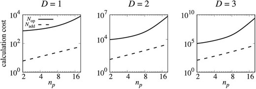
Values of N_add and N_op plotted against n_p. The dashed and solid lines show these values for N_add and N_op. From left to right, the values of D are 1, 2, and 3.

Open in new tab Download slide

3 Numerical experiments

In this section, we present the result of the Sod shock tube test in subsection 3.1 and that for the test of the surface gravity wave in subsection 3.2. We compare the results of fourth-order Hermite schemes and second- and fourth-order Runge–Kutta schemes in the Sod shock tube test, and the results of an fully implicit Hermite-scheme, the implicit fourth-order Runge–Kutta scheme, and the backward-Euler scheme in the surface gravity wave test.

3.1 Sod shock tube

In this section, we present the result of the Sod shock tube test (Sod 1978). We assume that fluid is an ideal gas with γ = 1.4. The computational domain is −0.5 ≤ x < 0.5 with a periodic boundary, and the initial boundary of two fluids are at x = −0.5 and 0. In this test, we used equal-mass particles. The initial velocity is given by |$v$|_x = 0. The density is smoothed by a C⁵ polynomial, and is given by

\begin{eqnarray} \rho (x) = \left\lbrace \begin{array}{ll}\rho _{\rm h} & -0.25 \le x < -x_0, \\ \frac{\rho _{\rm h} - \rho _{\rm l}}{2}\sum _{m=0}^5 b_m x^{2m+1} + \frac{\rho _{\rm h} + \rho _{\rm l}}{2} & -x_0 \le x < x_0,\\ \rho _{\rm l} & x_0 \le x \le 0.25, \end{array} \right.\nonumber\\ \end{eqnarray}

(49)

where (b₀, b₁, b₂, b₃, b₄, b₅) = (−693/256, 1155/256, −693/128, 495/128, −385/256, 63/256), and ρ_h and ρ_l are the values of initial density in the high- and low-density regions. We used ρ_h = 1 and ρ_l = 0.25. The parameter x₀ represents the width of the smoothing region, and we used two values of x₀. One is an initial condition with x₀ = 0.006, and the other is a smooth initial condition with x₀ = 0.03. We set the initial condition for 0.25 ≤ x < 0.5 to mirror that of 0 < x ≤ 0.25, and −0.5 ≤ x ≤ −0.25 as mirroring −0.25 ≤ x ≤ 0. The positions of particles in the smoothing region are determined so that position x_i of particle i satisfies

\begin{eqnarray} \int ^{x_i}_{x_{i-1}} \rho (x) dx = \frac{1}{2N_{\rm h}}, \end{eqnarray}

(50)

where N_h is the number of particles in the high-density region and the right-hand side of equation (50) is the mass of a particle. The smoothed pressure is given by

\begin{eqnarray} P(x) = \left\lbrace \begin{array}{ll}P_{\rm h} & -0.25 \le x < -x_0, \\ \frac{P_{\rm h} - P_{\rm l}}{2}\sum _{m=0}^5 b_m x^{2m+1} + \frac{P_{\rm h} + P_{\rm l}}{2} & -x_0 \le x < x_0,\\ P_{\rm l} & x_0 \le x \le 0.25, \end{array} \right. \end{eqnarray}

(51)

where P_h and P_l are the values of initial pressure in the high- and low-density regions. We used P_h = 1 and P_l = 0.1795. We used equations (31) and (32) for the artificial viscosity with h_AV = 2.375 × 10⁻³. We used a sixth-order interpolation with the value of interpolation polynomial at the position of particle |$\boldsymbol{x}_i$| fixed to the actual value. Therefore, |$\boldsymbol{\delta }$| given by equation (36) and |$\boldsymbol{p}_{ij}$| given by equation (36) are

\begin{eqnarray} \boldsymbol{\delta } &=& \left(1, \nabla _x, \frac{1}{2!}\nabla _x^2, \frac{1}{3!}\nabla _x^3, \frac{1}{4!}\nabla _x^4, \frac{1}{5!}\nabla _x^5 \right)^{T}, \end{eqnarray}

(52)

\begin{eqnarray} \boldsymbol{p}_{ij} &=& \left(1,x_{ij}, x_{ij}^2, x_{ij}^3, x_{ij}^4, x_{ij}^5\right)^{T}. \end{eqnarray}

(52)

The kernel function is the fourth-order Wendland function (Wendland 1995). The kernel length is given by

\begin{eqnarray} h_i &=& \eta \left(\frac{\tilde{m}_i}{\rho _i}\right)^{1/D}, \end{eqnarray}

(54)

\begin{eqnarray} \tilde{m}_i &=& \rho _{t=0,i} \Delta V_{t=0,i}, \end{eqnarray}

(55)

where ρ_{t = 0, i} and ΔV_{t = 0, i} are the density and geometric volume, respectively, of a particle i at t = 0. We set η = 3.8.

We calculated the L1-norm error of density at t = 0.1 to verify the spatial order of the schemes and to compare the accuracy of the schemes;

\begin{eqnarray} \epsilon _{\rho } = \sum _{n=1}^{N_x}\frac{1}{N_x} \frac{|\rho _n - \rho _{n}^{\mathrm{hres}}|}{\rho _{n}^{\mathrm{hres}}}, \end{eqnarray}

(56)

where |$\rho _{n}^{\mathrm{hres}}$| is the result of a high-resolution test in which the number of particles, N_x, is 8000 and dt = 10⁻⁶. When we derived equation (56), we calculated ρ_n of particles rearranged at the same positions as those of the high-resolution test. The time integrator for high-resolution test is the Hermite scheme of the P(EC)² form. For the test of the time order of the scheme for the test with N_x = N₀, |$\rho _{n,\Delta {t}}^{\mathrm{hres}}$| is the result of a high-resolution test in which N_x is N₀ and dt = 10⁻⁶. The time integrator for the high-resolution test is the same as that for ρ_n. In this case we define the error as

\begin{eqnarray} \epsilon _{\rho ,\Delta {t}} = \sum _{n=1}^{N_x}\frac{1}{N_x} \frac{|\rho _n - \rho _{n,\Delta {t}}^{\mathrm{hres}}|}{\rho _{n,\Delta {t}}^{\mathrm{hres}}}. \end{eqnarray}

(57)

We compare results with PEC, PECE, and P(EC)² forms of Hermite schemes, and Heun’s scheme (hereafter RK2) and the classical fourth-order Runge–Kutta scheme (hereafter RK4). The numbers of particles, N_x, are 1000, 2000, and 4000. Calculation codes used in this study were developed using FDPS (Iwasawa et al. 2016).

Figure 2 shows density profiles at t = 0.1 for the tests with N_x = 1000 and dt ≃ dt_max/4, where dt_max is the maximum time-step in the stability region, with the PEC form of the Hermite scheme. Note that the results for all schemes are similar to that for the PEC form of the Hermite scheme. We can see that the shock wave can be captured. However, the post-shock oscillation is strong for x₀ = 0.006. Figure 3 is the same as figure 2, but for N_x = 4000. Note that the results are independent of the time-integration scheme used and the results for N_x = 2000 are similar to those for N_x = 4000. We can see that the shock wave can be captured clearly even if the initial condition is not smooth. Therefore, if the initial condition is not smooth, the resolution of time and space should be higher.

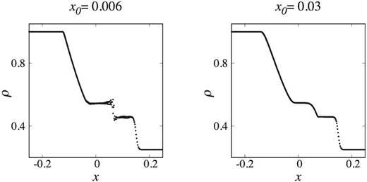
Results of the Sod shock tube tests with Nx = 1000. The density profiles at t = 0.1 are shown. The left- and right-hand panels show the results for x0 = 0.006 and x0 = 0.03.

Fig. 2.

Results of the Sod shock tube tests with N_x = 1000. The density profiles at t = 0.1 are shown. The left- and right-hand panels show the results for x₀ = 0.006 and x₀ = 0.03.

Open in new tab Download slide

Fig. 3.

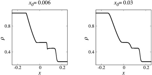
Same as figure 2, but for N_x = 4000.

Open in new tab Download slide

Now we check the spatial order of the scheme. We used the sixth-order shape function and then the first and second derivatives are fifth and fourth orders in space. Therefore, if the result converges to an exact solution following the order of the method, the order of the scheme should be larger than or equal to 4, and thus ε_ρ should be given by |$\epsilon _{\rho } \propto N_x^{-m}$| where m is larger than or equal to 4. Figure 4 shows that ε_ρ for the P(EC)² form of the Hermite scheme for runs with dt = 10⁻⁶ plotted against |$N_x^{-1}$|⁠. The results are independent of the time-integration scheme used. The value of ε_ρ for runs with x₀ = 0.006 is proportional to |$N_x^{-4}$|⁠. The value of ε_ρ in the large N_x region for runs with x₀ = 0.03 is proportional to |$N_x^{-1}$| since, in this region, the round-off error dominates the total error. In the other region, ε_ρ is proportional to |$N_x^{-4}$|⁠. From these results, we can conclude that the spatial order of the scheme is consistent with theoretical expectation.

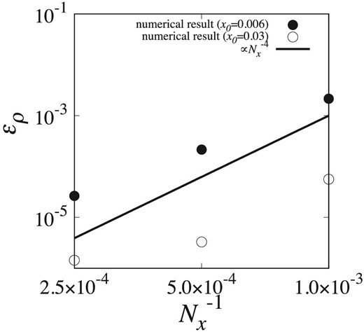
$ερ at t = 0.1 for the tests with x0 = 0.006 and x0 = 0.03 plotted against $N_x^{-1}$. Filled and open circles show results for x0 = 0.006 and 0.03, and the solid curve shows the theoretical models for the error.$

Fig. 4.

ε_ρ at t = 0.1 for the tests with x₀ = 0.006 and x₀ = 0.03 plotted against |$N_x^{-1}$|⁠. Filled and open circles show results for x₀ = 0.006 and 0.03, and the solid curve shows the theoretical models for the error.

Open in new tab Download slide

Let us look at the time orders of the schemes. Figures 5 and 6 show ε_{ρ, Δt} for the tests with x₀ = 0.006 and x₀ = 0.03 plotted against dt_ic, where dt_ic is dt divided by the number of interaction calculations per time step. We can see that the errors of RK2 and RK4 are |$\mathcal {O}(dt^2)$| and |$\mathcal {O}(dt^4)$|⁠, respectively, and that of the Hermite schemes is |$\mathcal {O}(dt^2)$|⁠.

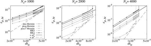
ερ, Δt at t = 0.1 for the tests with x0 = 0.006 plotted against dtic. From left to right, panels show the results for the Nx = 1000, 2000 and 4000. Triangles, squares and crosses show the results for Hermite schemes in PEC, PECE, P(EC)2 forms, and open and filled circles show the results for RK4 and RK2. Solid and dashed curves show the theoretical models for the error of second- and fourth-order schemes.

Fig. 5.

ε_{ρ, Δt} at t = 0.1 for the tests with x₀ = 0.006 plotted against dt_ic. From left to right, panels show the results for the N_x = 1000, 2000 and 4000. Triangles, squares and crosses show the results for Hermite schemes in PEC, PECE, P(EC)² forms, and open and filled circles show the results for RK4 and RK2. Solid and dashed curves show the theoretical models for the error of second- and fourth-order schemes.

Open in new tab Download slide

Same as figure 5, but the results for x0 = 0.03.

Fig. 6.

Same as figure 5, but the results for x₀ = 0.03.

Open in new tab Download slide

In the following we explain the reason why the order of the Hermite scheme is |$\mathcal {O}(dt^2)$| for fixed |$N_x^{-1}$|⁠. In a particle-based method, the calculated spatial derivatives contain discretization errors, and therefore the time derivative contains errors. In the case of RK schemes, this error causes the solution in the limit of dt → 0 to converge to a solution that is different from the exact solution, but the rate of the convergence is the order of the time-integration scheme, since we can regard the space-discretized differential equations as the set of ordinal differential equations. However, in the case of the Hermite scheme, we construct the second time-derivatives of physical quantities from the original equations and high-order spatial derivatives, and these spatial derivatives contain discretization errors. Thus, both the first and second time-derivatives contain the errors due to space discretization errors, and therefore the second time-derivatives are not exactly the time derivatives of the first time-derivatives. For simplicity, let us illustrate this behaviour for the integration of velocity in one dimension. Here, we rewrite the correctors by substituting equations (6) and (7) to equation (9). Note that we set dt = Δt in equation (4):

\begin{eqnarray} {v}_c &=& {v}_n + \frac{1}{2}({a}_{n} + {a}_{n+1})\Delta t + \frac{1}{12}({j}_{n} - {j}_{n+1})\Delta t^2. \end{eqnarray}

(58)

If we use sixth-order polynomial fitting for deriving spatial derivatives, |$v$|_c containing the spatial errors is given by

\begin{eqnarray} {v}_c = {v}_n + \frac{1}{2}\left({A}_{n} + {A}_{n+1}\right)\Delta t + \frac{1}{12}\left({J}_{n} - {J}_{n+1}\right)\Delta t^2, \end{eqnarray}

(59)

where A_n and A_{n + 1} are accelerations at n and n + 1 steps and J_n, and J_{n + 1} are jerks at n and n + 1 steps, all given by sixth-order polynomial fitting for deriving spatial derivatives. Therefore, J is not equal to the time derivative of A:

\begin{eqnarray} J = \frac{dA}{dt} + \epsilon _{J}, \end{eqnarray}

(60)

where ε_J is the error. Here, we integrate equation (59) from t = 0 to t = T,

\begin{eqnarray} {v}_{c,(t=T)} &=& {v}_{(t=0)} + \sum _{n=0}^{N_t}\left[\frac{1}{2}\left({A}_{n} + {A}_{n+1}\right)\Delta t\right] \nonumber \\ && + \sum _{n=0}^{N_t}\left[\frac{1}{12}\left({J}_{n} - {J}_{n+1}\right)\Delta t^2\right] \nonumber \\ &=& {v}_{(t=0)} + \sum _{n=0}^{N_t}\left[\frac{1}{2}\left({A}_{n} + {A}_{n+1}\right)\Delta t\right] \nonumber \\ && + \sum _{n=0}^{N_t}\left[\frac{1}{12}\left(\frac{dA_n}{dt} + \epsilon _{J,n} - \frac{dA_{n+1}}{dt} - \epsilon _{J,n+1}\right)\Delta t^2\right],\nonumber \\ \end{eqnarray}

(61)

where N_t is given by N_t = T/Δt. Here, we can assume that

\begin{eqnarray} \frac{dv}{dt} = \lim _{\Delta t = 0} A. \end{eqnarray}

(62)

Therefore, equation (61) becomes

\begin{eqnarray} {v}_{(t=T)} &=& {v}_{A}(T) + \mathcal {O}(\Delta t)^4 + \frac{1}{12}\left[\epsilon _{J,(t=0)} - \epsilon _{J,(t=T)}\right] \Delta t^2, \end{eqnarray}

(63)

where |$v$|_A(T) is the analytical solution for the velocity which satisfies equation (62). We can see that the time order of a Hermite scheme is equal to two. From these results, we can conclude that the time orders of the schemes are consistent. The fact that the apparent error order of the Hermite scheme is 2 does not imply it is a second-order scheme, because when we simultaneously shrink the interparticle distance and time step, the error will be |$\mathcal {O}(dt^4)$| as expected. The second-order behaviour occurs only when the spatial error dominates the total error.

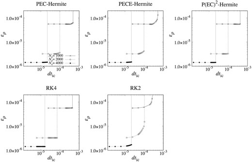
Figure 7 shows errors for tests with x₀ = 0.006 plotted against dt_ic. The result shows that the accuracy of fourth-order Hermite schemes is similar to those of RK2 and RK4, since the errors of spatial differentiation approximation determines the overall error.

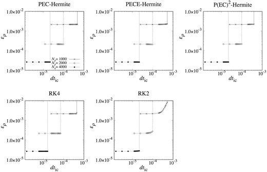
ερ at t = 0.1 for the tests with x0 = 0.006 plotted against dtic. From left to right in the upper panels, the results for the PEC-, PECE- and P(EC)2 forms of the Hermite schemes are shown. The lower left-hand and middle panels show the results for the second and fourth Runge–Kutta schemes. Crosses and open and filled circles show results for Nx = 1000, 2000, and 4000.

Fig. 7.

ε_ρ at t = 0.1 for the tests with x₀ = 0.006 plotted against dt_ic. From left to right in the upper panels, the results for the PEC-, PECE- and P(EC)² forms of the Hermite schemes are shown. The lower left-hand and middle panels show the results for the second and fourth Runge–Kutta schemes. Crosses and open and filled circles show results for N_x = 1000, 2000, and 4000.

Open in new tab Download slide

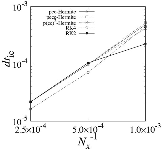
Figure 8 shows maximum dt_ic in the numerical stable region for tests with x₀ = 0.006 plotted against |$N_x^{-1}$|⁠. We can see that the regions of stability of fourth-order Hermite schemes are larger than or equal to those of RK2 and RK4. Hence, we can use larger time-steps with the Hermite schemes. Therefore, we can conclude that Hermite schemes, especially in PEC and PECE forms, are better than Runge–Kutta schemes for simulations of fluid with shock and contact discontinuity, even when the initial condition has a sharp jump.

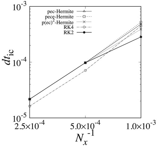
$Maximum dtic in the numerical stable region for tests with x0 = 0.006 plotted against $N_x^{-1}$. Triangles, squares, and crosses show the results for Hermite schemes in PEC, PECE, and P(EC)2 forms, and open and filled circles show the results for RK4 and RK2.$

Fig. 8.

Maximum dt_ic in the numerical stable region for tests with x₀ = 0.006 plotted against |$N_x^{-1}$|⁠. Triangles, squares, and crosses show the results for Hermite schemes in PEC, PECE, and P(EC)² forms, and open and filled circles show the results for RK4 and RK2.

Open in new tab Download slide

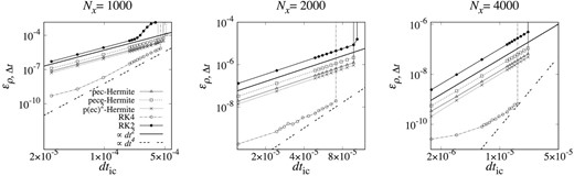
Figure 9 shows errors for x₀ = 0.03 plotted against dt_ic. As in the case of x₀ = 0.006, the results show that the accuracy of fourth-order Hermite schemes is similar to those of RK2 and RK4, since the errors of the spatial differentiation approximation determine the overall error.

Fig. 9.

Same as figure 7, but for x₀ = 0.03.

Open in new tab Download slide

Figure 10 shows maximum dt_ic in the numerical stable region for tests with x₀ = 0.03 plotted against |$N_x^{-1}$|⁠. As in the case of x₀ = 0.006, the results for the regions of stability of fourth-order Hermite schemes are larger than or equal to those of RK2 and RK4. Therefore, we can conclude that Hermite schemes, especially in PEC and PECE forms, are better than Runge–Kutta schemes for simulations of fluid with shock and contact discontinuity. We can conclude that Hermite schemes are more computationally efficient than Runge–Kutta schemes for calculation shocks.

Fig. 10.

Same as figure 8, but for x₀ = 0.03.

Open in new tab Download slide

3.2 Surface gravity wave test

The surface gravity wave test is useful for the investigation of the capability of numerical schemes to handle two-dimensional fluid dynamics with high accuracy and small dissipation. The initial condition is the same as those in Antuono et al. (2011) and Yamamoto and Makino (2017), but sound velocity given by equation (29) is 10 times smaller than that of Yamamoto and Makino (2017). We assume that fluid is weakly compressible with an equation of state given by equation (28) with ρ_air = 10³ and P_air = 10⁵ and sound velocity given by equation (29) with g = −10 and the height of fluid H = 1. The computational domain is 0 ≤ x < 1, 0 ≤ y ≤ 1. We applied a periodic boundary at x = 0, |$v$|_y = 0 at y = 0 and P = P_air for particles initially at y = 1 as boundary conditions. Initial density is

\begin{eqnarray} \rho (y) = \rho _{\mathrm{air}}e^{g(H-y)/c_0^2}. \end{eqnarray}

(64)

Initial velocity is

\begin{eqnarray} v_x &=& A\frac{|g|k}{\omega }\frac{\cosh (ky)}{\cosh (kH)}\sin (kx), \end{eqnarray}

(65)

\begin{eqnarray} v_y &=& -A\frac{|g|k}{\omega }\frac{\sinh (ky)}{\cosh (kH)}\cos (kx), \end{eqnarray}

(66)

where A, k, and ω are the amplitude, the wavenumber, and its frequency. We set A = 0.01, k = 2π, and |$\omega =\sqrt{|g|k\tanh (kH)}$|⁠. In this test, we do not use artificial viscosity to clarify the origin of the error. We used a fifth-order interpolation with the value of the interpolate polynomial at the position of particle |$\boldsymbol{x}_i$| fixed to the actual value.

Therefore, |$\boldsymbol{\delta }$| given by equation (36) and |$\boldsymbol{p}_{ij}$| given by equation (36) are

\begin{eqnarray} &&\boldsymbol{\delta } = \left(1, \nabla _x, \frac{1}{2!}\nabla _x^2, \nabla _x\nabla _y, \frac{1}{2!}\nabla _y^2, \dots , \frac{1}{2!3!}\nabla _x^2\nabla _y^3,\right.\nonumber\\ &&\left.\qquad\quad \frac{1}{4!}\nabla _x\nabla _y^4, \frac{1}{5!}\nabla _y^5 \right)^{T}, \end{eqnarray}

(67)

\begin{eqnarray} \boldsymbol{p}_{ij} &=& \left(1,x_{ij}, y_{ij}, x_{ij}^2, x_{ij}y_{ij}, y_{ij}^2, \dots , x_{ij}^2y_{ij}^3, x_{ij}y_{ij}^4, y_{ij}^5\right)^{T}. \end{eqnarray}

(68)

The kernel function is the fourth-order Wendland function (Wendland 1995). We used equation (54) as the kernel length and set η = 3.8.

We calculate the absolute error of |$v$|_x at (x, y) = (0.4, 1) and t = 0.2T where T is the period given by 2π/ω for checking the spatial order of the schemes and comparing the accuracy of the schemes.

\begin{eqnarray} \epsilon _{v_x} = {|v_{x} - v_{x}^{\mathrm{hres}}|}, \end{eqnarray}

(69)

where |$v_{x}^{\mathrm{hres}}$| is the result of the high-resolution test in which the number of particles, N, is 128 × 129 and dt = T/1024. The time integrator for high-resolution test is the implicit Hermite scheme. For checking the time order of the scheme for the test with N = N₀, |$v_{x,\Delta {t}}^{\mathrm{hres}}$| is the result of a high-resolution test in which N is N₀ and dt = T/512. The time integrator for a high-resolution test is same as |$v$|_x. We calculated |$v$|_x and |$v_{x,\Delta {t}}^{\mathrm{hres}}$| of the particles initially at (x, y) = (0.3125, 1). In this case we define the error as

\begin{eqnarray} \epsilon _{v_x, \Delta {t}} = {|v_{x} - v_{x,\Delta {t}}^{\mathrm{hres}}|}. \end{eqnarray}

(70)

We compare results of runs with the implicit Hermite scheme, the backward-Euler scheme (hereafter IRK1) and the Gauss–Legendre scheme (hereafter IRK4). The numbers of particles, N, are 16 × 17, 32 × 33, and 64 × 65.

Figure 11 shows the time evolution up to t = 0.75T with the implicit Hermite scheme, N = 16 × 17 and dt ≃ dt_max/4. Figure 12 shows y of the particle initially at (x, y) = (0, 1) with the implicit Hermite scheme, N = 16 × 17 and dt ≃ dt_max/4. Note that the results are independent of the time-integration scheme used and N.

Fig. 11.

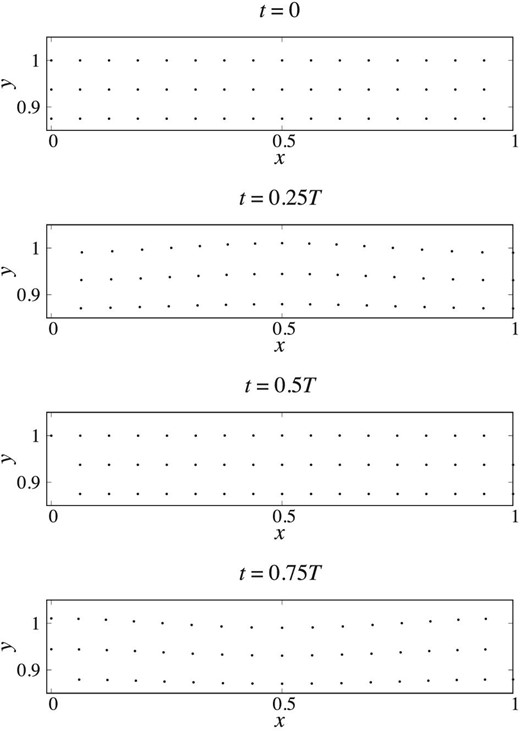
Results of the surface gravity wave tests with N = 16 × 17; from top to bottom, the snapshots at t = 0, 0.25T, 0.5T, and 0.75T are shown.

Open in new tab Download slide

Fig. 12.

Time-evolution of the y-coordinate of the particle initially at (x, y) = (0, 1) in the surface gravity wave test with N = 16 × 17.

Open in new tab Download slide

Now we check the spatial order of the scheme. We used the fifth-order shape function and then the first and second derivatives are fourth and third orders in space. Therefore, if the result converges to an exact solution following the order of the method, the order of the scheme should be larger than or equal to 3, and thus |$\epsilon _{v_x}$| should be given by |$\epsilon _{v_x} \propto N_x^{-m}$| where m is larger than or equal to 3 and N_x is the number of particles in the x-direction. Figure 13 shows |$\epsilon _{v_x}$| for the implicit Hermite scheme with dt = T/512 plotted against |$N_x^{-1}$|⁠. We can see that the error |$\epsilon _{v_x}$| is proportional to |$N_x^{-4}$|⁠. Therefore, the error in acceleration determines the overall error. The results are independent of the time integration used. From the result, the spatial order of the scheme is consistent.

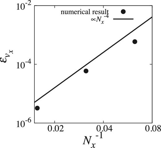
$$\epsilon _{v_x}$ at t = 0.2T plotted against $N_x^{-1}$. Filled circles show numerical results and solid curves show the theoretical models for the error.$

Fig. 13.

|$\epsilon _{v_x}$| at t = 0.2T plotted against |$N_x^{-1}$|⁠. Filled circles show numerical results and solid curves show the theoretical models for the error.

Open in new tab Download slide

Let us now look at the time order of the scheme. Figure 14 shows |$\epsilon _{v_x, \Delta {t}}$| plotted against dt_ic. We can see that the errors of the implicit Hermite scheme, IRK4, and IRK1 are |$\mathcal {O}(dt^2)$|⁠, |$\mathcal {O}(dt^4)$|⁠, and |$\mathcal {O}(dt)$|⁠, respectively. As described in subsection 3.1, the time order of the Hermite scheme is equal to 2. From these results, we can conclude that the time orders of the schemes are consistent.

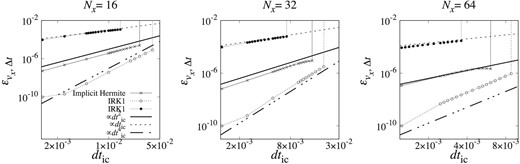
$$\epsilon _{v_x, \Delta {t}}$ plotted against dtic. From left to right, panels show the results for the Nx = 16, 32 and 64. Crosses and open and filled circles show the results of the implicit Hermite scheme, IRK4, and IRK1. Dashed, solid and treble-dot–dashed curves show the theoretical models for the error of second-, first-, and fourth-order schemes.$

Fig. 14.

|$\epsilon _{v_x, \Delta {t}}$| plotted against dt_ic. From left to right, panels show the results for the N_x = 16, 32 and 64. Crosses and open and filled circles show the results of the implicit Hermite scheme, IRK4, and IRK1. Dashed, solid and treble-dot–dashed curves show the theoretical models for the error of second-, first-, and fourth-order schemes.

Open in new tab Download slide

Figure 15 shows errors plotted against dt_ic. The result shows that the accuracy of the implicit Hermite scheme is similar to that of IRK4 and smaller than that of IRK1 with large N.

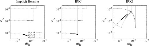
$$\epsilon _{v_x}$ plotted against dtic. Left-hand, middle and right-hand panels show the results for the implicit Hermite scheme, IRK4, and IRK1. Crosses and open and filled circles show results for Nx = 16, 32, and 64.$

Fig. 15.

|$\epsilon _{v_x}$| plotted against dt_ic. Left-hand, middle and right-hand panels show the results for the implicit Hermite scheme, IRK4, and IRK1. Crosses and open and filled circles show results for N_x = 16, 32, and 64.

Open in new tab Download slide

Figure 16 shows the maximum dt_ic in the numerical stable region plotted against |$N_x^{-1}$|⁠. We can see that the region of stability of the implicit Hermite scheme is wider than those of IRK1 and IRK4. Hence, we can use larger time-steps with the implicit Hermite scheme. Therefore, we can conclude that the Hermite scheme is better than Runge–Kutta schemes for simulations of fluid with the surface and gravity wave.

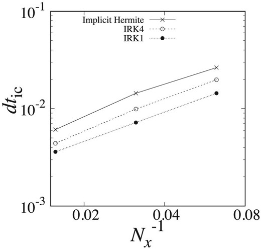
$dt ic in the numerical stable region for tests with x0 = 0.006 plotted against $N_x^{-1}$. Crosses and open and filled circles show the results of the implicit Hermite scheme, IRK4, and IRK1.$

Fig. 16.

dt _ic in the numerical stable region for tests with x₀ = 0.006 plotted against |$N_x^{-1}$|⁠. Crosses and open and filled circles show the results of the implicit Hermite scheme, IRK4, and IRK1.

Open in new tab Download slide

4 Summary

If we use multi-stage integration schemes, such as Runge–Kutta schemes, with mesh-free methods we need to perform the interaction calculation, which is the most expensive part of the calculation, multiple times per time step. We constructed a Hermite scheme for a high-order mesh-free method. The accuracy of fourth-order Hermite schemes is at least similar to those of Runge–Kutta schemes and the region of stability of Hermite schemes is better than those of Runge–Kutta schemes. Therefore, we can use a large time-step with the Hermite scheme compare to that for the Runge–Kutta scheme for the same accuracy. We conclude that Hermite schemes are more computationally efficient than commonly used Runge–Kutta schemes for a high-order mesh-free method.

Acknowledgements

We would like to thank the referee for his or her insightful comments and suggestions. We also thank the editor for his or her assistance. We thank Masaki Iwasawa, Keigo Nitadori and Daisuke Namekata for discussions about Hermite schemes and Runge–Kutta schemes. This research was supported by RIKEN Junior Research Associate Program and MEXT as “Exploratory Challenge on Post-K computer” (Elucidation of the Birth of Exoplanets [Second Earth] and the Environmental Variations of Planets in the Solar System).

References

Antuono

M.

,

Colagrossi

A.

,

Marrone

S.

,

Lugni

C.

2011

,

Comput. Phys. Commun.

,

182

,

866

Crossref

Search ADS

Aoki

T.

1997

,

Comput. Phys. Commun

.,

102

,

132

Crossref

Search ADS

Iwasawa

M.

,

Tanikawa

A.

,

Hosono

N.

,

Nitadori

K.

,

Muranushi

T.

,

Makino

J.

2016

,

PASJ

,

68

,

54

Crossref

Search ADS

Makino

J.

1991

,

ApJ

,

369

,

200

Crossref

Search ADS

Makino

J.

,

Aarseth

S. J.

1992

,

PASJ

,

44

,

141

Sod

G. A.

1978

,

J. Comput. Phys.

,

27

,

1

Crossref

Search ADS

Wendland

H.

1995

,

Adv. Comput. Math.

,

4

,

389

Crossref

Search ADS

Yamamoto

S.

,

Makino

J.

2017

,

PASJ

,

69

,

35

Crossref

Search ADS

This article is published and distributed under the terms of the Oxford University Press, Standard Journals Publication Model (https://dbpia.nl.go.kr/journals/pages/open_access/funder_policies/chorus/standard_publication_model)

Download all slides

Month:	Total Views:
December 2018	2
January 2019	9
February 2019	15
March 2019	4
April 2019	4
May 2019	5
June 2019	1
August 2019	2
September 2019	5
October 2019	6
November 2019	1
December 2019	3
January 2020	1
March 2020	1
June 2020	3
August 2020	1
September 2020	1
January 2021	9
February 2021	10
March 2021	7
April 2021	8
May 2021	7
June 2021	4
July 2021	6
August 2021	5
September 2021	8
October 2021	10
November 2021	3
December 2021	3
January 2022	7
February 2022	5
March 2022	21
April 2022	7
May 2022	10
June 2022	3
July 2022	9
August 2022	9
September 2022	15
October 2022	10
November 2022	3
December 2022	5
January 2023	11
February 2023	8
March 2023	3
April 2023	9
May 2023	8
June 2023	8
July 2023	2
August 2023	12
September 2023	6
October 2023	10
November 2023	7
December 2023	13
January 2024	15
February 2024	6
March 2024	10
April 2024	13
May 2024	5
June 2024	10
July 2024	12
August 2024	16
September 2024	10
October 2024	10
November 2024	2
December 2024	5
January 2025	11
February 2025	9
March 2025	5
April 2025	5
May 2025	3

Article Contents

Hermite integrator for high-order mesh-free schemes

Abstract

1 Introduction

2 Derivation of the high-order scheme

2.1 Hermite scheme

2.2 Derivation of high-order time-derivatives for hydrodynamical equations

2.3 Calculation cost for high-order time-derivatives

3 Numerical experiments

3.1 Sod shock tube

3.2 Surface gravity wave test

4 Summary

Acknowledgements

References

Citations

Views

Altmetric

Email alerts

Astrophysics Data System

Citing articles via

Latest

Most Read

Most Cited

Article Contents

Hermite integrator for high-order mesh-free schemes Free

Abstract

1 Introduction

2 Derivation of the high-order scheme

2.1 Hermite scheme

2.2 Derivation of high-order time-derivatives for hydrodynamical equations

2.3 Calculation cost for high-order time-derivatives

3 Numerical experiments

3.1 Sod shock tube

3.2 Surface gravity wave test

4 Summary

Acknowledgements

References

Citations

Views

Altmetric

Email alerts

Astrophysics Data System

Citing articles via

Latest

Most Read

Most Cited

This Feature Is Available To Subscribers Only

Hermite integrator for high-order mesh-free schemes