


Abstract
Archival NuSTAR data of the magnetar 4U 0142+61, acquired in 2014 March for a total time span of 258 ks, were analyzed. This is to reconfirm the 55 ks modulation in the hard X-ray pulse phases of this source, found with a Suzaku observation in 2009 (Makishima et al., 2014, Phys. Rev. Lett., 112, 171102). Indeed, the 10–70 keV X-ray pulsation, detected with NuSTAR at 8.68917 s, was found to be also phase-modulated (at >98% confidence) at the same ∼55 ks period, or half that value. Furthermore, a brief analysis of another Suzaku data set of 4U 0142+61, acquired in 2013, reconfirmed the same 55 ks phase modulation in the 15–40 keV pulses. Thus, the hard X-ray pulse-phase modulation was detected with Suzaku (in 2009 and 2013) and NuSTAR (in 2014) at a consistent period. However, the modulation amplitude varied significantly; A ∼ 0.7 s with Suzaku (in 2009), A ∼ 1.2 s with Suzaku (in 2013), and A ∼ 0.17 s with NuSTAR. In addition, the phase modulation properties detected with NuSTAR differed considerably between the first 1/3 and the latter 2/3 of the observation. In energies below 10 keV, the pulse-phase modulation was not detected with either Suzaku or NuSTAR. These results reinforce the view of Makishima et al. (2014, Phys. Rev. Lett., 112, 171102); the neutron star in 4U 0142+61 keeps free precession, under a slight axial deformation due probably to ultra-high toroidal magnetic fields of ∼1016 G. The wobbling angle of precession should remain constant, but the pulse-phase modulation amplitude varies on time scales of months to years, presumably as asymmetry of the hard X-ray emission pattern around the star’s axis changes.
1 Introduction
In Paper I (see figure 3b therein) and Makishima (2016), we interpreted the above Suzaku results in the following way.
- The NS in this system is axially symmetric; its moment of inertia I3 around the symmetry axis |$\hat{x}_3$| (to be identified with the magnetic dipole axis) differs slightly from that in orthogonal directions, I1. The deformation is specified by asphericity, defined as(2)\begin{equation} \epsilon \equiv (I_1 - I_3)/I_3. \end{equation}
The NS, being axisymmetric, undergoes free precession. The |$\hat{x}_3$| axis rotates around the constant angular momentum |$\boldsymbol{L}$| with the precession period Ppr ≡ 2πI1/L, keeping a constant wobbling angle α to |$\boldsymbol{L}$|. At the same time, the NS rotates around |$\hat{x}_3$| with the rotation period Prot ≡ 2πI3/L. The observed pulse period should be identified with Ppr rather than Prot.
- The beat between Ppr and Prot defines a long period atwhich is called the slip period. Substituting equation (1) for this T, and assuming cos α ≈ 1, we obtain(3)\begin{equation} T \equiv \left[(1/P_{\rm rot} - 1/P_{\rm pr}) \cos \alpha \right]^{-1} = P_{\rm pr}/( \epsilon \cos \alpha ) , \end{equation}(4)\begin{equation} \epsilon =P_{\rm pr}/(T \cos \alpha ) \approx P_{\rm pr}/T =1.6 \times 10^{-4}. \end{equation}
If the emission pattern is axially symmetric around |$\hat{x}_3$|, we would detect periodicity at neither Prot nor T. This condition is thought to apply to the SXC pulsation, of which the pulse phase is not modulated.
If the X-ray emission pattern, in contrast, breaks symmetry around |$\hat{x}_3$|, the pulse arrival times (and hence the pulse phase) become modulated at T. This is thought to explain the behavior of the HXC pulses. If the degree of this asymmetry varies, the modulation amplitude A will differ among observations, even though α should remain constant.
- We regard the deformation as prolate (ε > 0), in which case the free precession should develop spontaneously. Such a prolate deformation as equation (4) can in turn be caused by strong toroidal MF Bt hidden inside the NS, as(Cutler 2002; Ioka & Sasaki 2004). Hence the NS in 4U 0142+61 is suggested to harbor Bt ∼ 1016 G, which exceeds by two orders of magnitude its nominal dipole MF of Bd = 1.3 × 10¹⁴ G (Gavriil & Kaspi 2002).(5)\begin{equation} \epsilon \sim 1\times 10^{-4} (B_{\rm t}/10^{16}\:\mbox{G})^2 \end{equation}
The Suzaku discovery deserves further studies, because the effect potentially provides vital information on the internal MF of magnetars, which is otherwise difficult to measure. Actually, we have discovered a second example, the highly variable and fastest-rotating magnetar 1E 1547.0−5408. In this case, the Suzaku data obtained in its 2009 January outburst revealed that the hard X-ray pulses with Ppr = 2.0721 s are phase-modulated at a period of T = 36 ks (Makishima et al. 2016, hereafter Paper II). Again assuming cos α ∼ 1, equation (3) yields ε = 0.6 × 10⁻⁴, which is of the same order as equation (4) for 4U 0142+61.
Since the above results have all been obtained with Suzaku, we evidently need to study this intriguing phenomenon using other X-ray observatories. Actually, Tendulkar et al. (2015), hereafter TEA15, searched the NuSTAR data of 4U 0142+61 acquired in 2014 March for the same phase-modulation effects, and found no evidence over a range of T = 45–65 ks. However, as already suggested by the multiple Suzaku data (item 5 above), A would vary as the anisotropy of the HXC emission pattern changes (with α kept constant). It is hence important to re-examine the NuSTAR data for evidence of pulse-phase modulation, at a period consistent with equation (1), but allowing for different values of A. With these in mind, we re-analyze the same NuSTAR data as TEA15 used.
2 Observation
As described by TEA15, 4U 0142+61 was observed with NuSTAR in 2014 March in two successive pointings. The first, shorter, one (ObsID 30001023002) was from 2014 March 27 UT 13:35 to March 28 UT 00:45, for a gross exposure of 41 ks and a net exposure of 24 ks. The second and longer one (ObsID 30001023003) immediately followed the first one, and lasted from March 28 UT 00:45 to March 30 UT 13:01. The achieved gross and net exposures are 217 and 144 ks, respectively.
In the present work, the two data sets are co-added for our analysis, to cover an overall time span of 258 ks (a net exposure of 168 ks). The events taken with the two focal-plan modules, FPMA and FPMB, are also co-added together. We accumulated on-source events within a circle of radius 60′ around the image centroid, because the signal-to-noise ratio of the source was maximized at a radius of 60′ to 70′ in the 20–70 keV range, which plays an important role in our study. Then, subtracting the background and applying dead-time and vignetting corrections, the object was detected at a 4–70 keV count rate of 1.009 ± 0.002 counts s−1 for FPMA+FPMB. Finally, like in TEA15, the event arrival times were photon-by-photon converted to those to be measured at the solar system barycenter; this utilized the source position of (αJ2000.0, δJ2000.0) = (|${01{^\rm{h}}46{^\rm{m}}22{^\rm{s}_{.}}41}$|, 61°|${45^{\prime}03{^{\prime\prime}_{.}}2}$|), as well as the spacecraft orbital information.
3 Data analysis and results
3.1 Basic analyses
3.1.1 Light curves
Figure 1 shows dead-time-corrected but background-inclusive light curves of 4U 0142+61 with 5 ks binning. Here and hereafter, the overall energy range is subdivided into three; 4–10 keV, 10–20 keV, and 20–70 keV, to be called L, M, and H bands, respectively. The energy range below 4 keV (down to the nominal lower bound of 3 keV) was discarded to avoid any possible drifts in the detector’s lower threshold. Similarly, we discard the highest energy interval of 70–78 keV, because of the reduced effective area therein. The L band covers the SXC, whereas M and H mainly represent the HXC. Using the 60′ event accumulation radius, the background amounts to approximately 1.2%, 5.2%, and 32% of the total counts in L, M, and H, respectively.
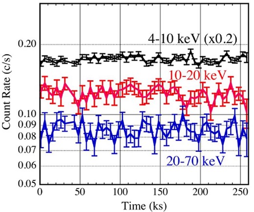
Background-inclusive light curves in the 4–10 keV (L; black), 10–20 keV (M; red), and 20–70 keV (H; blue) bands, all binned into 5 ks. Error bars are ±1σ. The L-band data are multiplied by a factor of 0.2 for presentation. (Color online)
In figure 1, the assumption of a constant count rate gives χ2/ν = 1.52, 1.21, and 1.12 in the L, M, and H bands, respectively, all for ν = 50. Therefore, some intrinsic intensity variations are suggested in the L band (with a null hypothesis probability of 1%), and possibly in the M band (7.5%) as well, but the H band variations are dominated by Poisson fluctuations.
3.1.2 Hardness ratios
In figure 1, the M and H count rates show a hint of anti-correlation, even though their intrinsic variations are not so significant (sub-subsection 3.1.1). This is suggestive of changes in the HXC slope. We hence produced time histories of two hardness ratios, (M + H)|$/$|L and H/M, which can be seen in figure 2. The former, i.e., the HXC vs. SXC intensity ratio shown in green, is found to be consistent with being constant within errors. The latter, representing the HXC slope, in contrast exhibits more noticeable variations. Actually, after applying the 3-bin running average (25%, 50%, and 25% weights for three consecutive data points), it yields χ2/ν ∼ 2.0 (ν ∼ 25) against the constant-value hypothesis, with an implied null-hypothesis probability of ∼0.2%. Here, we considered that the employed running average approximately halves both the total noise power and the effective degrees of freedom. Thus, the HXC slope exhibits statistically significant variation, in agreement with the M vs. L anti-correlation suggested by figure 1.
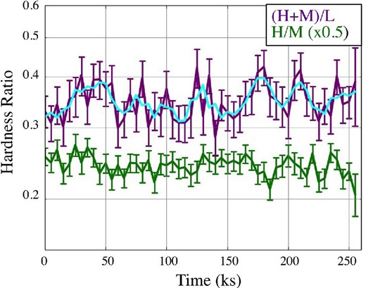
Time histories of the two hardness ratios, (M + H)/L (green) and M/H (purple), with ±1σ error bars. The former is halved for presentation. The cyan curve superposed on the latter shows the result of 3-bin running average. (Color online)
The variations in the H|$/$|M ratio seen in figure 2 are not only significant, but also appear rather periodic, with a period of 5–6 bins (25–30 ks). We hence Fourier-analyzed the two hardness ratios in figure 2, as well as the three-band light curves in figure 1. The obtained five power spectra are presented in figure 3. Thus, in the H|$/$|M power spectrum (purple), the power reaches ∼14.48 at a wavenumber of q = 9, or a period of ∼258/q ∼ 28.7 ks, which is consistent with just half the period of equation (1). In addition, some power enhancements are seen at q ∼ 5 (period of ∼52 ks) which could be a subharmonic. To evaluate the significance of the q = 9 peak, we must consider the fact that the average of the H|$/$|M power spectrum (excluding k = 0) reaches 4.14, which is 2.07 times higher than the value of 2.0 expected for a purely Poisson-dominated case. Therefore, the source is varying in the H|$/$|M ratio. Regarding the value of 4.14 as a quadratic sum of the Poissonian fluctuations and this intrinsic source variation, and assuming the latter to have a white spectrum, we renormalized the power at q = 9 to 14.48/2.07 = 7.00, to obtain a chance probability of 1.5% for this peak. The probability becomes rather high, ∼38%, when multiplied by the overall wave numbers of 25 to take into account so-called “look-elsewhere effects”. However, if we limit our search to the first two (fundamental and the second) harmonics and the 1/2 subharmonic of equation (1), the probability still remains ∼4.5%, and hence the peak is significant at a confidence of ∼90% or higher. A related further discussion on this point is given in subsection 3.3.
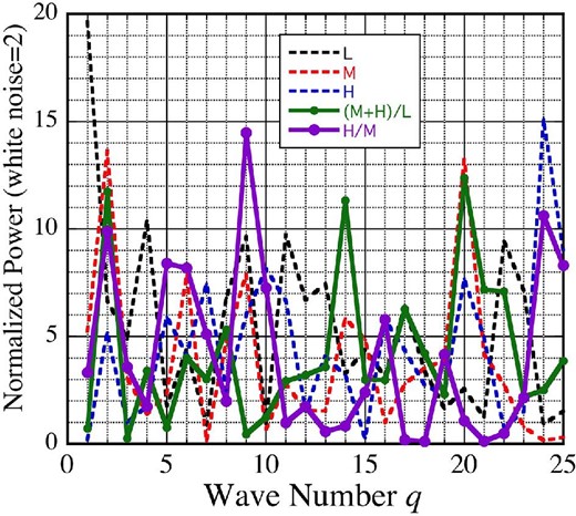
Fourier power spectra, calculated from the three light curves in figure 1 and the two hardness ratios in figure 2. They are all normalized so that the power becomes 2.0 when the statistical white noise dominates. Their colors are the same as in figure 1 and figure 2. The wavenumber q has a period of 258/q ks. (Color online)
We hence conclude that the HXC of 4U 0142+61 observed with NuSTAR exhibits some evidence of spectral-slope variations at a period that is consistent with half the period of equation (1).
3.1.3 Pulsations
In the present study, we search the data for periodicities using the |$Z_N^2$| analysis (Buccheri et al. 1983; Brazier 1994; Enoto et al. 2011; Paper I; Paper II; see also sub-subsection 3.2.1). By applying this method to the background-inclusive 10–70 keV events, with the harmonic number set at N = 3 (see below), the 8.69 s source pulsation was detected throughout the observation. Since the local pulse period obtained from the first 6 ks (gross) of data could be inconsistent with (shorter than) those from the other intervals, we exclude, unless otherwise stated, this first 6 ks from the subsequent data analysis throughout the present study, although the origin of this effect is unclear. Our major results remain unchanged even if this time range is retained.
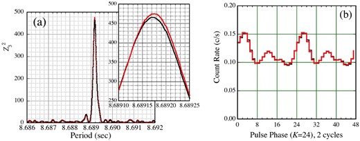
(a) |$Z_3^2$| pulse periodogram of 4U 0142+61, calculated using the background-inclusive 10–70 keV NuSTAR data. Black and red are before and after the demodulation analysis, and the inset gives a blow-up around the peak. (b) Folded 10–70 keV pulse profile, before (black) and after (red) the demodulation, smoothed with 3-bin running average. The background is inclusive, and the count rate is corrected for neither deadtime nor vignetting. The statistical 1 σ error is about ±0.003 counts s−1. (Color online)
The black trace in figure 4b shows the background-inclusive 10–70 keV pulse profile, folded at equation (6). Here and hereafter, the present work employs the time origin as 2014 March 27, UT 13:36:18.551, before the barycentric correction is applied. The profile is double-peaked, with the primary and secondary peaks, in agreement with TEA15. Since the two peaks are separated in phase by about 0.37 cycles, rather than 0.5, the profile must include harmonics higher than N = 2. In fact, by Fourier-transforming the profile, we found that the power in the fundamental (N = 1), the second (N = 2), the third, and the fourth harmonics carry about 32%, 53%, 9%, and 2% of the total power (including the Poissonian noise), respectively. Therefore, below we basically adopt N = 3, even though N = 4 was used in Paper I.
3.2 Demodulation analysis
The study has now come to the stage of examining whether the periodicity of equation (1), found with Suzaku, is also present in the NuSTAR data. For this purpose, we apply the demodulation analysis, developed in Paper I and Paper II, to the NuSTAR data.
3.2.1 Procedure
First, we select a trial value of T, and sort the 10–70 keV events (including background) into a two-dimensional array C(j, k); here, j = 1, 2, .., J − 1 specifies the phase in T, J is the total phase number in T, k = 1, 2, .., K − 1 is the pulse phase variable (i.e., the time modulo P), and K is the overall pulse-phase bin number. After an appropriate exposure correction, {C(j, k); k = 0, 1, .., K − 1} gives the folded pulse profile at the jth phase of the period T. This procedure may be called double folding.
3.2.2 Results in 10–70 keV
The analysis described above has been applied to the 10–70 keV NuSTAR data, where the search scans were performed over T = 20–120 ks with a step of 0.2–2 ks, A = 0–0.25 s with a 0.01 s step, and ψ0 = 0°–360° with a 5°–10° step; P was scanned over the error range of equation (6) with a 5-μs step. We employed the Z2 harmonic number of N = 3 (sub-subsection 3.1.3), and large values of J = 90 and K = 360 to make the results in equation (8) insensitive to J and K. Unless ambiguous, |$Z_N^2$| is hereafter abbreviated as Z2.
The derived results are summarized in figure 5, which is the same plot as figure 2 of Paper I and figure 4 of Paper II except for some stylistic changes. The solid purple curve in panel (a), to be called a demodulation periodogram (as distinguished from pulse periodograms such as figure 4a) displays the maximum value of Z2, obtained at each T while scanning in P, A, and ψ0 over the specified ranges. At T ∼ 55 ks, which is of our prime interest, we indeed observe a clear peak. As indicated by the dashed green trace in the same panel (a), the modulation amplitude that maximizes Z2 also increases to A ∼ 0.17 s around this modulation period. These results suggest that the pulse-phase modulation effects detected with Suzaku are also present in the NuSTAR data, although the amplitude is much reduced.
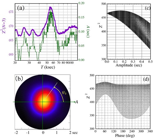
Results of the demodulation analysis on the 10–70 eV (M + H) NuSTAR data using N = 3, where |$Z_{\,3}^{\,2}$| is abbreviated as Z2. (a) The maximum value of Z2 (purple, left-hand ordinate) found at each T. The dashed green trace (right-hand ordinate) shows the values of A that maximized Z2. (b) A color-scale presentation of Z2 on the (A, ψ0) polar coordinates, for a particular period of T = 55 ks. The phase ψ0 is measured anti-clockwise from due right. (c) The projection of panel (b) on to the A axis, which is shown by a green arrow in panel (b). (d) That on the phase (ψ0) axis, which is indicated in panel (b) in yellow. (Color online)
In figure 5a, we also observe a few smaller Z2 enhancements, including those at T ∼ 110 ks and T ∼ 27 ks, which are just twice and half the 55 ks period, respectively. They are also accompanied by some increases in A. Hereafter, the 55 ks and 27 ks humps seen in these demodulation periodograms are called Zp55 and Zp27, respectively.
Parameters of the 55 ks and 27 ks humps in the 10–70 keV |$Z_N^2$| periodograms.
| Zp55 (= hump at T ∼ 55 ks) | Zp27 (= hump at T ∼ 27 ks) | |||||||||||
|---|---|---|---|---|---|---|---|---|---|---|---|---|
| Time range | N * | (Z2)0 | T (ks) | Z 2 | ΔZ2 | A (s) | ψ0 (°) | T (ks) | Z 2 | ΔZ2 | A (s) | ψ0 (°) |
| 3 | 465.94 | 54.8 ± 5.3 | 476.83 | 10.89 | 0.17 ± 0.08 | 60 ± 30 | 26.2 ± 1.7 | 469.55 | 3.61 | 0.10 ± 0.05 | 330 ± 60 | |
| All | 7 | 474.50 | 54.3 ± 5.1 | 483.67 | 9.17 | 0.15 ± 0.09 | 50 ± 30 | 25.4 ± 2.1 | 480.28 | 5.78 | 0.14 ± 0.07 | 340 ± 60 |
| 3m | 398.18 | 56.6 ± 4.6 | 415.96 | 17.78 | 0.24 ± 0.09 | 50 ± 30 | 26.4 ± 2.5 | 406.55 | 8.37 | 0.14 ± 0.05 | 300 ± 60 | |
| 3 | 143.40 | — | — | — | — | — | 26.4 ± 3.1 | 148.01 | 4.61 | 0.20 ± 0.12 | 300 ± 40 | |
| TR-1 | 7 | 149.36 | — | — | — | — | — | 25.4 ± 2.6 | 173.98 | 24.62 | 0.39 ± 0.17 | 310 ± 30 |
| 7m | 137.41 | — | — | — | — | — | 26.4 ± 2.9 | 166.36 | 28.95 | 0.38 ± 0.18 | 310 ± 30 | |
| 3 | 331.45 | 54.5 ± 6.2 | 343.91 | 12.46 | 0.20 ± 0.11 | 60 ± 50 | — | — | — | — | — | |
| TR-2 | 7 | 341.40 | 54.4 ± 7.6 | 352.76 | 11.36 | 0.22 ± 0.11 | 80 ± 50 | — | — | — | — | — |
| 3m | 282.82 | 55.0 ± 7.3 | 299.85 | 17.03 | 0.24 ± 0.10 | 50 ± 60 | — | — | — | — | — | |
*The Z2 hadmonic number, with “m” meaning that the secondary pulse peak is masked out as described in subsection 3.5.
When the demodulation is carried out, the 10–70 keV pulse periodogram and the folded pulse profile changed as shown in red in figure 4a and figure 4b, respectively. The difference between “before” and “after” is however very small, reflecting the rather small increment ΔZ2.
The demodulation analysis was repeated by chaining N from 3 upwards. Generally, the |$\Delta Z_N^2$| value for Zp55 did not change very much. However, that for Zp27 increased up to |$\Delta Z_{10}^2 \sim 8$| at N ∼ 10, beyond which the Poisson noise started to affect the demodulation periodogram. This intriguing effect is further studied in sub-subsection 3.2.4. As representative cases of higher N, the parameters derived with N = 7 are given in the second row of table 1.
3.2.3 Visualization of the pulse-phase modulation
Even though Zp55 is observed rather clearly in figure 5a, the rather small increment in Z2, namely, ΔZ2 = 10.89 ≪ (Z2)0, might cast some doubts on its reality. Thus, to visualize the suggested effect, figure 6a shows the 10–70 keV double-folding map C(j, k) (sub-subsection 3.2.1) in a gray scale. It was produced using Ttot = 252 ks, T = 55 ks, and P0 of equation (6), and is presented with J = 6 and K = 30 after applying the 3-bin running average to the k (abscissa) dimension. We have chosen these particular values of K and J as a compromise between sufficient statistics and adequate time resolution. There, the double-peaked pulse profile (figure 4b) appears as two ridges per cycle, running almost vertically. In addition, the phase modulation is observed as a slight wiggling of the primary (brighter) ridge by ±1 bin, corresponding to A ∼ ±P0/30 = ±0.29 s. This map is to be compared with the soft X-ray result in figure 11 to be presented later, wherein no pulse-phase modulation is observed at T ∼ 55 ks.
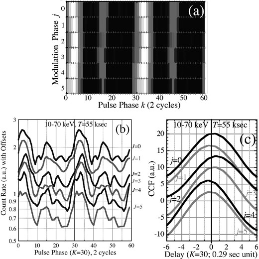
Visualization of the 10–70 keV pulse-phase modulation. (a) A gray-scale count-rate map C(j, k) obtained by double-folding the 10–70 keV data using T = 55 ks, P0 of equation (1), J = 6, and K = 30. Abscissa shows the pulse phase k for 2 cycles, and ordinate represents the 55 ks modulation phase j, from top to bottom, for one cycle. (b) The 10–70 keV folded pulse profiles for different j, shown in semi-logarithmic scale with vertical offsets. (c) CCFs of the pulse profiles for j = 0, 1, ... 5, from top to bottom. They were calculated as described in text, and are shown in arbitrary units with vertical offsets. Abscissa is the time lag in units of P0/30 = 0.29 s, where positive values mean delays behind the template.
Figure 6b shows the pulse profiles {C(j, k): k = 0, 1, 2, ..,} at individual modulation phases j; it is just another way of presenting panel (a). To make the primary and secondary peaks both visible, the ordinate utilizes a logarithmic scale. We reconfirm that the primary pulse peak is modulated, as a function of j, by approximately the same amount as in panel (a).
At each j, we cross-correlated the profile in panel (b), against an average pulse profile (summed over j) which is shown in red in figure 4b. The same J = 6 and K = 30 as panels (a) and (b) were used. The obtained cross-correlation functions (CCFs) are presented in figure 6c, where the smoothing method described in Paper I was incorporated. Again, the correlation peak moves back and forth, by ∼±0.5 unit in this presentation, or A ∼ ±0.15 s, which is consistent with equation (12). However, it is smaller than the amplitude, A ∼ 0.3 s, visible in figure 6a and figure 6b. This issue is further considered in subsection 3.5.
3.2.4 Time evolution of the modulation effects
It is known that the pulse profiles of 4U 0142+61 (Enoto et al. 2011; Archibald et al. 2017) and of some other magnetars (e.g., Kuiper et al. 2012; Coti Zelati et al. 2017) change on a time scale of a day or longer. To see whether the demodulation periodogram changed across the three days covered by the present observation, we divided the gross time span of 252 ks into two time ranges, the first 1/3 (about 80 ks in gross after removing the first 6 ks) to be called Time Range 1, hereafter TR-1, and the latter 2/3 (about 172 ks) to be called Time Range 2 or TR-2. Thus, TR-1 and TR-2 cover the first day and the latter two days, respectively. This particular time division is justified later.
In figure 7a, the solid lines in red and blue give the N = 3 demodulation periodograms derived from TR-1 and TR-2, respectively. They were calculated over T = 10–100 ks, because of the shorter data span. Surprisingly, Zp55 seen in figure 5a appears only in TR-2 (blue solid line), whereas Zp27 appears mainly in TR-1 (red solid line). The parameters of these humps are summarized in table 1. We ignore the structures at ∼12 ks, which could be instrumental because they are close to twice the orbital period (5.8 ks) of NuSTAR.

Demodulation analyses applied to the two time ranges, TR-1 and TR-2. (a) The 10–70 keV demodulation periodograms from TR-1, with N = 3 (solid red) and N = 7 (dashed orange), and those from TR-2, with N = 3 (solid dark blue) and N = 7 (dashed cyan). (b) The folded 10–70 keV pulse profiles from TR-1. The black one is before demodulation, whereas the red one is after demodulation using the corresponding parameters given in table 1 with T = 55 ks. Unlike figure 4, ordinates are truncated below 0.08 counts s−1. (c) The same as panel (b), but for TR-2.
Given the possible N-dependence of Zp27 (sub-subsection 3.2.2), we repeated the same time-divided analysis by changing N. Then, as shown in figure 7a by a dashed orange line, Zp27 in TR-1 became drastically stronger, until it saturated at ΔZ2 = 24.62 with N = 7. As given in table 1, the amplitude also became considerably larger than in equation (12). In contrast, as shown by a dashed cyan line in figure 7a, Zp55 in TR-2 did not change significantly over N = 3–7. The widths of these Z2 humps generally satisfy equation (10). For reference, table 1 also lists the Zp55 and Zp27 information when the N = 7 demodulation is applied to the total 252 ks of data.
The different N-dependences in TR-1 and TR-2, as found above, and rather unexpectedly, suggest that the 10–70 keV pulse profile in TR-2 is smoother, whereas that in TR-1 is more structured, with rich, higher harmonic structures that have been smeared out through the pulse-phase modulation. To examine this inference, we present in panels (b) and (c) of figure 7 the folded pulse profiles derived separately from the two time ranges. The raw profile from TR-2 [black in panel (c)] is similar to the time-averaged one in figure 4, and changes only slightly (blue) after the demodulation using the Zp55 parameters given in table 1 (row with TR-2 and N = 3). Here and hereafter, the demodulation procedure employs T = 55.0 ks for Zp55 and T = 27.5 ks for Zp27 as fiducial numbers, considering the latter as half the former. In contrast, the pulse profile from TR-1 [black in panel (b)] has a more square-wave like shape, and its edges become sharper (the red profile) via demodulation using the Zp27 parameters in table 1 (row with TR-1 and N = 7). These results agree with the expectation from figure 7a.
The time-evolution effects are further visualized in figure 8, where the double-folding maps, like figure 6a, are presented separately for TR-1 (left two panels) and TR-2 (right two panels). The TR-2 data, when folded at T = 55 ks [panel (c)], approximately reproduce the phase modulation seen in figure 6a, but such effects are not observed when folded at T = 27.5 ks [panel (d)] at least in the primary pulse. The TR-1 data, in contrast, shows a clear phase modulation at T = 27.5 ks [panel (b)], which appears also as a hint of two-cycle modulation in panel (a) where T = 55 ks is employed. These results reconfirm figure 7.
![Same double-folding results of the 10–70 keV photons as figure 6a, but derived from TR-1 [panels (a) and (b)] and TR-2 [panels (c) and (d)]. Panels (a) and (c) employ the folding period of T = 55 ks in the ordinate direction, whereas panels (b) and (d) use T = 27.5 s.](https://oup.silverchair-cdn.com/oup/backfile/Content_public/Journal/pasj/71/1/10.1093_pasj_psy129/3/m_pasj_71_1_15_f12.jpeg?Expires=1749222562&Signature=XzQIeJq7-Si3DLK5Iztmkyh1~oRDshcrAjMlNcFtEvxuCB~9SLXBvlq94vOx3pOo8NRpTUZAQXoLmSVILSJ0f54nIZ4ZskJQp0IfyeubB8NNGhif9ELfuQopx0cHfQ7UnSooQEKp~X4G5FMEzQis8dS4RefkYOL3sxI-xHqGHvAhYDkidyNA4sv36NGa9XAgRhjZruVuEHcn0vsKnsKyUeIbTIfh5Lr9LAWLqiIPMZ5~KRjef4fTw28tDqAiJaszSgQDIjDagMfYhQbRbOreug1HnFi5G2CVNkoG2v46hcXKfT5Lz9XWrBHotzXvGb~ksViZ59K8dero61xJOPX6GA__&Key-Pair-Id=APKAIE5G5CRDK6RD3PGA)
Same double-folding results of the 10–70 keV photons as figure 6a, but derived from TR-1 [panels (a) and (b)] and TR-2 [panels (c) and (d)]. Panels (a) and (c) employ the folding period of T = 55 ks in the ordinate direction, whereas panels (b) and (d) use T = 27.5 s.
The phase-modulation properties thus changed rather drastically from TR-1 to TR-2, accompanied by some changes in the pulse profile. Nevertheless, a comparison between panels (b) and (c) of figure 7 reveals no significant difference in the average 10–70 keV intensity, or the pulse fraction.
3.3 Significance of the phase modulation
Although we have so far obtained evidence that the 10–70 keV pulses are phase-modulated at 55 ks, or just half that value, the increments ΔZ2 in table 1 could be due simply to statistical fluctuations, because Z2 would fluctuate through equation (8) via different superpositions of the Poisson noises on all pixels of C(j, k). To examine this issue, we may adopt a null hypothesis that the pulse phase is intrinsically not modulated at a given period T beyond Poissonian fluctuations, and estimate the statistical chance probability |${\cal P}_{\rm dem}$| for such noise superpositions to make ΔZ2 at that T higher than a specified value.
Since our aim is to confirm the Suzaku results rather than to discover a new modulation period (cf. sub-subsection 3.1.2), the estimation of |${\cal P}_{\rm dem}$| can be made for a single value of T, neglecting the look-elsewhere effects, unlike the cases of Paper I and Paper II. This is because the range of T in equation (12) is represented by a single wavenumber as q = 4.6 ± 0.4 (for Ttot = 252 ks), and hence is effectively covered by a single independent value of T in reference to equation (10). With this in mind, below we estimate |${\cal P}_{\rm dem}$| for Zp55 in two different ways, both using the actual data themselves. Monte Carlo simulations are not employed, because we encounter difficulties in properly modeling the intrinsic intensity variations (figure 1) and the known pulse-profile changes (Enoto et al. 2011).
As the first attempt, we performed the N = 3 demodulation analysis, over a range of T = 0.7–5.0 ks, which is much longer than P0 but shorter than the NuSTAR’s orbital period, 5.8 ks. This control study utilized the entire data length (but the first 6 ks), and the same scan procedures in P, A, and ψ0 as in figure 5. The scan steps in T were chosen to follow equation (10), to make the results with different T mutually independent. We thus conducted 300 steps in T, and confirmed that the ΔZ2 values from adjacent sampling points of T are uncorrelated. As a result, |$\Delta Z_3^2$| exceeded the target value of |$\Delta Z_3^2=10.89$| (table 1) in four realizations among the 300 trials; this yields |${\cal P}_{\rm dem} \sim 1.3\%$|. More quantitatively, figure 9a shows the upper probability integral of the 300 values, derived by integrating their distribution from the largest towards smaller values. The probability at first decreases as ∝ exp (−ΔZ2/2.0) (the dashed line), as expected for a chi-square distribution of any degree of freedom (Paper II) at ΔZ2 ≪ (Z2)0, and then it starts exhibiting some excess at ΔZ2 > 3, presumably reflecting the source variability. This plot yields |${\cal P}_{\rm dem} \sim 2\%$|, which agrees with the above simple-minded calculation.
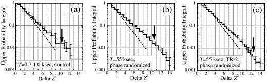
Estimated upper probability integrals for ΔZ2 of equation (11) in 10–70 keV. The dashed line indicates the slope expected for a chi-square distribution at ΔZ2 ≪ (Z2)0, and the vertical arrow shows ΔZ2 given in table 1. (a) An estimation based on 300 independent control trials over T = 0.7–5 s. (b) That based on 3000 independent trials, all employing T = 55 ks, and incorporating the phase randomization (see text). (c) The same as panel (b), but for Zp55 in the N = 3 demodulation periodogram from TR-2.
As the second attempt, we followed Paper II, and repeated the N = 3 demodulation analysis of the 252 ks data, employing the same (P, A, ψ0) volume and the same parameter steps, but fixing the value T = 55 ks and ignoring the look-elsewhere effect. Furthermore, in each trial, we performed a random permutation as {j = 0, 1, .., J − 1} → {j′ = 0, 1, .., J − 1}, and replaced {C(j, k)} with {C(j′, k)} (i.e., a random permutation of rows in figure 6a), before equation (8) and equation (9) are executed. Different trials employed different realizations of the permutation, all with J = 90. This phase randomization would bring any possible intrinsic phase modulation at T to a level that is consistent with Poissonian fluctuations. Furthermore, all these permutations must be statistically equivalent, because the Poisson noise in different pixels of C(j, k) should be independent (Paper II). As a result, we can study the behavior of Z2 under the null hypothesis presented above. We have thus executed 3000 trials, and found 42 cases in which |$\Delta Z_3^2$| exceeded |$\Delta Z_3^2=10.89$|. More quantitatively, figure 9b shows the upper probability integral, thus derived from the 3000 trials. It indicates |${\cal P}_{\rm dem} \sim 2\%$|, in a good agreement with the first evaluation. We also confirmed that |${\cal P}_{\rm dem}$| is unchanged even employing different but similar values of T (e.g., 50 ks).
The latter of the above two evaluations was applied also to TR-2, again with T = 55 ks fixed and N = 3. The results, shown in figure 9c, imply |${\cal P}_{\rm dem} \sim 0.5\%$| for Zp55 in this time range [blue curve in figure 7a]. The more stringent value of |${\cal P}_{\rm dem}$| obtained here is mainly due to the higher target value of |$Z_3^2=12.46$|, because the upper probability curve is more or less similar to that in panel (b).
Finally, the same randomization analysis, but with N = 7, was applied to the TR-1 data, to evaluate the significance of Zp27 seen in figure 7a. Since the modulation period in this case is less well known in advance, we scanned over T, from 25.0 to 28.5 ks with a step of 0.5 ks. Then |$\Delta Z_7^2$| exceeded the target value of 24.62 in only four out of the 3000 trials. We hence obtain |${\cal P}_{\rm dem} \sim 0.1\%$|, which is rather conservative (due to the T scan) but still sufficiently small because of the very prominent Zp27 in the N = 7 demodulation periodogram from TR-1.
In summary, Zp55 has a chance probability of |${\cal P}_{\rm dem} \sim 2\%$| if the entire data are used, and |${\cal P}_{\rm dem} \sim 0.5\%$| if TR-2 is concerned. Furthermore, Zp27 in TR-1 has a considerably lower chance probability as |${\cal P}_{\rm dem} \sim 0.1\%$|. All these values assume that the modulation period is known in advance from the Suzaku result.
3.4 Energy-dependent effects
3.4.1 Data in the 10–17.5 and 17.5–70 keV bands
To examine the phase-modulation phenomenon for possible energy dependence, we subdivided the 10–70 keV band into two bands, one at 10–18 keV (called M’) and the other at 18–70 keV (called H’). Choosing the boundary at 18 keV, instead of 20 keV, is simply to make the pulse significance in terms of Z2 about the same between M’ and H’; the results described below do not change very much if using the original M and H bands.
The demodulation analysis in the M’ and H’ bands, using the 252 ks data length and N = 3, yielded the results presented in figure 10a in red and blue, respectively. Thus, Zp55 is seen in both demodulation periodograms, and is stronger in H’. Within errors, the hump centers in M’ and H’ are both consistent with equation (12). In contrast, Zp27 is seen only in M’. Instead, the H’ band data exhibits some other enhancements, at 22 ks, 33 ks, and 42 ks. Among them, the 22 ks feature is likely to be caused by background variations, because it appears just at 4 times the NuSTAR’s orbital period, and is much stronger in H’ than in M’. The 33 ks peak can be interpreted as a beat between Zp55 in the data, and the one-day periodicity which dominates the data-sampling window; i.e., 1/55 + 1/86.4 = 1/33.6. Finally, the one at 42 ks is probably a beat between Zp55 and two days (172.8 ks). The 33 ks and 42 ks features are also stronger in H’ than in M’, probably because these beat effects can be enhanced when Poisson fluctuations of comparable strengths are added in quadrature to the intrinsic beat signal.
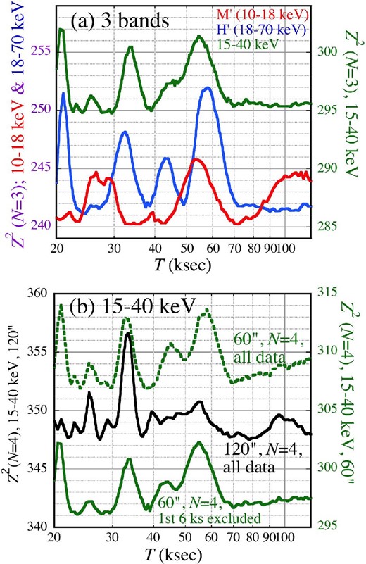
(a) Demodulation periodograms obtained from 10–18 keV (M’; red, left-hand abscissa), 18–70 keV (H’; blue, also left-hand abscissa), and 15–40 keV (green, right-hand abscissa), all using the same analysis conditions as in figure 5a. (b) Detailed comparison with TEA15, in the 15–40 keV range. The solid green curve (right-hand abscissa) is the same as that in panel (a), but using N = 4 instead of N = 3. The result changes as in the dotted green curve, when the first 6 ks is restored. Black (left-hand abscissa) shows the N = 4 result in 15–40 keV using the event accumulation radius of 120′, to reproduce the condition of TEA15. (Color online)
3.4.2 Consistency with Tendlukar et al. (2015)
Analyzing the same NuSTAR data over the 15–40 keV range (the same conditions as in Paper I), TEA15 found no evidence for the pulse-phase modulation at any period between 45 ks and 65 ks, including in particular 55 ks. To cross-check their report, we applied the demodulation analysis to the 15–40 keV data, using the same analysis conditions and the same parameter search steps (including 0.01 s in A) as in figure 5. The result is shown in green in figure 10a. There, we still find Zp55, though with a reduced height due presumably to the narrower energy range.
Although the above finding might appear inconsistent with TEA15, our analysis conditions still differ from those of TEA15 in several points. In fact, TEA15 used N = 4 instead of our N = 3, and they did not discard the first 6 ks. More importantly, they used the event accumulation region of 120′ radius (vs. ours of 60′), so their data have larger background contributions, which are estimated to be 16% in M and 64% in H. To progressively better reproduce the conditions employed by TEA15, we first changed from N = 3 to N = 4, and obtained the solid green curve in figure 10b. Its behavior is very similar to the case of N = 3 in panel (a), except for a systematic increase in Z2 by 1.5–2, which is reasonable. Next, we restored the first 6 ks of the data, and obtained the dotted green periodogram in panel (b). Thus, the inclusion/exclusion of the first 6 ks systematically changes the |$Z^2_3$| values by ∼12, but no other significant differences are noticed. Finally, we extracted FPMA + FPMB events within 120′ of the image centroid, instead of 60′, and applied the demodulation analysis to the 15–40 keV data with N = 4. Then, as shown in black in figure 10b, the Z2 values generally increased by 35–40 due to the increased signal photons, but Zp55 became no longer visible, probably buried by increased statistical fluctuations. Instead, the beat at 33 ks (which was outside the range searched by TEA15) increased significantly, presumably again due to a coupling between the intrinsic 55 ks periodicity and larger background fluctuations. Under such conditions, a beat could sometimes dominate over the original signal.
We have thus reproduced the essential point by TEA15, and confirmed the consistency between the two studies. The overall comparison can be interpreted in the following way. In the Suzaku observation, the signal-to-noise ratio of the demodulation periodogram was optimized by selecting a relatively limited energy band (15–40 keV) to reduce background, because the HXD is a non-imaging device, and yet the modulation amplitude was rather large (A ∼ 0.7 s; Paper I) on that occasion. In the present case, in contrast, the difficulty in confirming the 55 ks modulation lies primarily in the very small value of A. In addition, the sensitivity with NuSTAR, being an imaging instrument, would be optimized by widening the signal-acceptance energy band, and by choosing a narrow event accumulation region to suppress the background.
3.4.3 Analysis of lower-energy data
It is important to examine whether Zp55 and Zp27 are also present in the SXC, which dominates the energies below ∼10 keV. We hence performed the same demodulation analysis with N = 3, using the 4–6.1 keV photons. This particular energy range was chosen because the value of (Z2)0 = 477.40 therein is close to that in the 10–70 keV range, enabling an easy comparison. The result, given in figure 11a, shows no evidence of significant Z2 increase at T ∼ 55 ks, although some structures are observed at T ∼ 27 ks and ∼31 ks. Tentatively, an upper limit of A < 0.1 s may be assigned, where 0.1 was taken as an average of errors in A in table 1, and also considering the behavior of A in 4–6.1 keV at T ∼ 55 ks. We obtain essentially the same result even when expanding the energy band into 4–10 keV, where we find Z2 ∼ 785 on average.
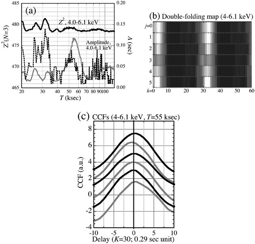
Results obtained from low-energy bands. (a) The N = 3 demodulation periodogram in 4–6.1 keV (solid curve), and the behavior of A (dashed curve). The 10–70 keV result, the same as in figure 5a, is superposed in gray. (b) The same double-folded map as figure 6a, but for the 4–6.1 keV signals. (c) The same CCFs as figure 6c, derived in the 4–6.1 keV range.
Panels (b) and (c) of figure 11 provide the same information as figure 6a and figure 6c, respectively, for the 252 ks of 4–6.1 keV signals. Because the pulse profile is nearly single-peaked in low energies (e.g., TEA15), a single ridge per cycle is observed in panel (b). No clear evidence of sinusoidal phase modulation at T = 55 ks is observed, either in panel (b) or (c), although the CCFs suggest some higher harmonic effects as already seen in figure 11a. This is possibly in line with figure 10, where it is suggested that Zp27 is softer than Zp55.
In short, the result obtained here agrees with the finding made in Paper I from 4U 0142+61 (and that in Paper II from 1E 1547−5408), that the phase modulation is seen only in the HXC.
3.5 The primary and secondary pulse peaks
The pulse profiles of 4U 0142+61 above 10 keV are double-peaked, consisting of primary and secondary peaks (figures 4b and 7). The demodulation results so far obtained for the HXC are considered to reflect mainly the behavior of the primary peak, because it is significantly stronger. To confirm this inference, we conducted the same analysis, but masking out the secondary peak; that is, after processing the data with equation (8) and equation (9), the pulse profile D(k) from k = 10 to k = 23 (for K = 30) in figure 6b (from 120° to 270° in the pulse phase) is replaced by the pulse-phase average of D(k), and then the Fourier transform is executed to calculate Z2. As listed again in table 1, this analysis has given results that are rather similar to figure 5 and figure 7. We therefore confirm that the results obtained in subsection 3.2 mainly reflect the behavior of the primary pulse peak.
On a closer look at table 1, both ΔZ2 and A of Zp55 are found generally to increase by masking out the secondary pulse peak. Therefore, the secondary pulse peak is likely to be free from the phase-modulation effects, and is partially canceling out the modulation specified by the primary peak. This may explain why the values of A of Zp55, which is ∼0.17 s from the demodulation periodogram in figure 5a and ∼0.15 s from the CCF in figure 6c, are smaller than those visually suggested by figure 6a and figure 6b.
For further examination, we tried to mask out the primary pulse peak, namely, k = 26 to k = 40 (for K = 30) in figure 6b. However, the reduced statistics did not allow us to obtain meaningful results.
4 Discussion
4.1 Summary of the NuSTAR results
Analyzing the NuSTAR data of 4U 0142+61 acquired in 2014, we have obtained the following results.
As in figure 5, the HXC pulses are phase-modulated, at a period of ∼55 ks [equation (12)] which is consistent with the Suzaku period of equation (1). When only the range of equation (1) is considered, employing N = 3, this peak, Zp55, is significant at 98% confidence if using the entire NuSTAR data, and at 99.5% if the time region is limited to TR-2 (subsection 3.3).
The phase-modulation amplitude associated with Zp55 is rather small, A ∼ 0.17 s, or A/P ∼ 0.02.
The data also exhibit Zp27 (figure 7a), i.e., an indication of HXC pulse-phase modulation at a period that is consistent with just half the value of equation (12) and equation (1).
From TR-1 to TR-2, neither the average 10–70 keV intensity nor the pulse fraction changed significantly. Nevertheless, Zp27 and Zp55 appeared essentially only in TR-1 and TR-2, respectively, involving some changes in the HXC pulse shapes (sub-subsection 3.2.4).
Particularly in TR-1, the Zp27 significance increased with N, from |$\Delta Z_3^2=4.61$| to |$\Delta Z_7^2=24.62$|, the latter implying 99.9% confidence. In contrast, the Zp55 significance depends little on N.
The 27 ks periodicity appears also in the power density spectrum of the H/M ratio, at a wavenumber q = 9 (figure 3). This q = 9 peak is significant at a confidence level of ∼90% or higher, if the look-elsewhere effects are ignored.
The negative detection of these effects by TEA15, using the same NuSTAR data, can be attributed primarily to the rather small value of A, augmented by the narrower energy band and the wider data accumulation radius they employed (sub-subsection 3.4.2).
While the primary peak of the HXC pulse is phase modulated, the secondary peak is probably not (subsection 3.5).
Below 10 keV where the SXC dominates, the pulse phase is modulated at neither ∼55 ks nor ∼27 ks, with a typical upper limit of A < 0.1 s (sub-subsection 3.4.3).
4.2 Brief (re-)analysis of the Suzaku data
To complement the results from NuSTAR, we conducted two brief (re-)analyses of the Suzaku data of 4U 0142+61.
One is a re-analysis of the 2009 Suzaku data, because the N = 4 demodulation periodogram in figure 2d of Paper I covered only 30 ≤ T ≤ 70 ks, without information at ∼27 ks. We hence repeated the same demodulation analysis as in Paper I, again using the 15–40 keV HXD data from 2009 with N = 4, but scanning T over a wider range of 20–120 ks and with a finer step of 0.2–2 ks than in Paper I; these parameters match those in the present NuSTAR study. The other parameters were scanned in the same way as in Paper I, namely, A = 0–1.2 s with a 0.1 s step, ψ0 = 0°–360° with a 10° step, and P = 8.68894–8.688904 s with a 5 μs step. The obtained results, shown in figure 12a, reproduce the data points in figure 2d of Paper I, and reconfirm the 55 ks peak, the parameters of which are summarized in table 2. We also notice a hint of a peak at T ∼ 27 ks, although its significance is not obvious.
![Suzaku results on the 15–40 keV pulse-phase modulation, obtained in 2009 [panel (a)] and 2013 [panel (b)], with the former updating figure 2d of Paper I. The solid curves show the $Z_4^2$ perodograms (left-hand ordinate), and the dashed curves the value of A (right-hand ordinate) that maximizes $Z_4^2$ at each T. The associated parameters are given in table 2.](https://oup.silverchair-cdn.com/oup/backfile/Content_public/Journal/pasj/71/1/10.1093_pasj_psy129/3/m_pasj_71_1_15_f4.jpeg?Expires=1749222562&Signature=DQjn6nbUpKO7dOjD16DBYFfmSiIiCmdMqvvHLKo0AHhrSQuDm9xOj1vfpI87tFGcdDvYLiRXkhw9hWwiEiNbA3nzVKtEBAKLO9DG514HaHTau1dmiZldnO4DwveSK20pndTFfljmSxj0gKHVgrGAWmVC6Ul9jALoV942iB20OFjImJrIyW7U-2DDao3VM5CZAq8~xWEeTiOMP2w7uLwL1T-TtMYoso-ESP8~rKlbkp~6EIfBcQQz2m59yaYde7ffnQjQ97qfZmsk5CIWeO0~sZh12j8OEUG1AZVQKApleXHBcDVka72oiRWalHyNT0d62NtPPpJbusTcBIlSbrNmtQ__&Key-Pair-Id=APKAIE5G5CRDK6RD3PGA)
Suzaku results on the 15–40 keV pulse-phase modulation, obtained in 2009 [panel (a)] and 2013 [panel (b)], with the former updating figure 2d of Paper I. The solid curves show the |$Z_4^2$| perodograms (left-hand ordinate), and the dashed curves the value of A (right-hand ordinate) that maximizes |$Z_4^2$| at each T. The associated parameters are given in table 2.
Parameters of the 55 ks peak in the demodulation periodograms from the four data sets.
| Data set | Exp. (ks) | Energy | N | Period* | |${(Z_N^2)_0}^\dagger$| | T | |$\Delta Z_N^2$| | A |
|---|---|---|---|---|---|---|---|---|
| Gross/Net | (keV) | (s) | (ks) | at T | (s) | |||
| Suzaku 2007 August‡ | 204/101 | 15–40 | 4 | 8.68878 | 52.01 | —|$^{\S}$| | —|$^{\S}$| | (|$<0.9)^{\S}$| |
| Suzaku 2009 August‡‖ | 186/102 | 15–40 | 4 | 8.68899 | 13.87 | 55 ± 4 | 25.63 | 0.7 ± 0.3 |
| Suzaku 2013 July–August‖ | 192/95 | 15–40 | 4 | 8.68914 | 16.36 | 54 ± 3 | 22.17 | 1.2 ± 0.4 |
| NuSTAR 2014 March | 258/168 | 10–70 | 3 | 8.68917 | 465.94 | 54.8 ± 5.3 | 10.89 | 0.17 ± 0.08 |
The other analysis concerns the Suzaku data of 4U 0142+61 obtained in 2013. Below, we concisely describe the observation and the obtained results, leaving further details to a later publication. Aiming to reconfirm the discovery described in Paper I, this follow-up Suzaku observation was conducted from 09: 46: 00 UT on 2013 July 31 to 15: 00: 00 UT on August 2, for exposures as given in table 2. The observing conditions and the source intensity were very similar to those in 2009. The pulsation was detected with the XIS at P = 8.68914 ± 0.00003 s, and the demodulation analysis was applied to the background-inclusive 15–40 keV HXD data with N = 4. We employed the same parameter search conditions as in figure 12a, except using a wider range of the amplitude scan: A = 0–1.5 s. The results are presented in figure 12b in the same manner as figure 12a and figure 5a, and the derived parameters are summarized in table 2. Thus, the 55 ks peak is clearly confirmed, with a slightly smaller ΔZ2 and a possibly larger A than in 2009. Furthermore, we observe a clear |$Z_4^2$| peak at T ∼ 27 ks. Like in 2009, the 1–10 keV pulses showed no evidence of phase modulation at 55 ks or 27.5 ks, with upper limits of A < 0.3 s considering the low time resolution of the XIS (Paper I).
4.3 Comparison with the Suzaku results
We are now ready to examine the nine items in subsection 4.1, through their comparison with the Suzaku results given in Paper I and subsection 4.2. First of all, item 1 on Zp55 agrees with the Suzaku achievements in 2009 and 2013. In fact, the value of T ∼ 55 is fully consistent among the three observations (table 2), and the three demodulation periodograms (figures 5a, 12a, and 12b) are strikingly similar, even though A is different. Another common property of the three data sets is the absence of these effects in the SXC (item 9). We hence conclude that the 55 ks pulse-phase modulation is not a Suzaku-specific artifact, but is an intrinsic property of 4U 0142+61 that is also observed with NuSTAR. The phenomenon is absent (or much weaker) in the SXC.
In Paper I, the chance probability was calculated as <1% for the 55 ks peak with |$\Delta Z_4^2=25.63$| (figure 12b, table 2) to appear at any period over T = 30–70 ks in the 2009 Suzaku data. In the present work, that of finding the 55 ks peak with ΔZ2 = 10.89 (table 1, table 2) in the NuSTAR data, at a consistent period, has been estimated as ≲2% (subsection 3.3). An evaluation similar to that in figure 9 yields a chance probability of ∼1 × 10⁻⁴ for the 2013 Suzaku data to show the Z2 peak with ΔZ2 = 22.17 (table 2) at the same period (figure 12b). Multiplying these three numbers, the overall chance probability to observe the 55 ks HXC pulse-phase modulation in the three observations can be reduced to ∼2 × 10⁻⁸.
Item 2 provides the largest difference of the present NuSTAR results, compared with those from Suzaku. Indeed, the value of A has decreased by 4 and 7 times from the 2009 and 2013 Suzaku observations, respectively, the latter only in less than a year from 2013 August to 2013 March (the present NuSTAR observation). The change of A, however, had already been noticed in Paper I, because the HXC pulse-phase modulation was absent in the Suzaku data acquired in 2007 (Enoto et al. 2011), when the observing conditions and the source intensity were both similar to those in 2009 and 2013. The results from the 2007 Suzaku observation are quoted in table 2.
In this regard, the present NuSTAR data resemble those of Suzaku in 2007, in which the HXC pulsation was detected significantly with |$(Z_4^2)_0=52.01$| for N = 4 (table 2), through the simple period search (Enoto et al. 2011) without considering the pulse-phase variations. In contrast, the HXC pulsation in the 2009 and 2013 Suzaku data was rather insignificant if employing such a conventional analysis, with |$(Z_4^2)_0=13.87$| (upper probability of 8.5%) in 2009 and |$(Z_4^2)_0=16.38$| in 2013 (3.7%). It was only after the application of the demodulation procedure that the HXC pulsation in these data sets were detected significantly, with Z2 > 38 (table 2), at the same period as the SXC pulsation. We thus conclude that A can vary considerably, on a time scale of months to years; sometimes A is so large as to smear out the HXC pulses (2009 and 2013), but on other occasions the effect is undetectable (in 2007) or detectable only through a very careful analysis of high-quality data, just as in the present case.
Another important effect found with NuSTAR is item 3, i.e., the appearance of Zp27 at about half the period of Zp55. Although this issue was not considered in Paper I, the reanalysis in figure 12a suggests its hint in the 2009 Suzaku data. Moreover, it is much more clearly seen in those of 2013 (figure 12b). The 27 ks periodicity is further supported by item 6, because the q = 9 peak in the power spectrum of the H|$/$|M ratio (figure 3) has a period which is consistent with T ∼ 27 ks. We hence conclude that the periodicity at ∼27 ks is another intrinsic property of this magnetar, and regard Zp27 as the second harmonic (in terms of frequency) of Zp55, even though the relation between the H|$/$|M variation and the pulse-phase modulation is not obvious.
Still more intriguing findings are item 4, i.e., the switching between Zp27 and Zp55, and item 5, i.e., the strong N-dependence of Zp27. Just as A of Zp55 is variable, the amplitude of Zp27 would also vary, either independently of that of Zp55, or in a mutually exclusive manner. Although we searched the 2009 and 2013 Suzaku data for similar effects, the results were inconclusive due to insufficient statistics.
4.4 Possible origins of the modulation
Our discussion has so far been purely empirical. Before conducting more physical interpretations in terms of free precession of a rigid body (subsection 4.5), we survey, once again, other possible explanations of what has been observed.
As argued in Paper I, the pulse-phase modulation with T = 55 ks and A = 0.7 s (the 2009 Suzaku parameters) could have been explained in the most natural way if the source formed a binary with a companion which has a mass 0.12 M⊙/sin i, where M⊙ is the solar mass and i the inclination. However, this interpretation is clearly ruled out, by the drastic change in A in 8 months, and the absence of the same modulation in the SXC. This conclusion, already derived in Paper I, has been much reinforced by the present study.
Supposing that 4U 0142+61 is an isolated NS, it could still be powered by accretion from a fall-back disk (e.g., Zezas et al. 2015). Then, a long periodicity could arise via precession of the assumed disk. As the disk precesses, the materials may be caught by different magnetic field lines of the NS, so that the accretion columns (emitting the HXC) could be slightly displaced, to produce a periodic shift in the pulse phase. Fluctuations of the disk conditions could change A. If, in addition, the SXC arises from the heated NS surface, its pulses would be free from phase jitters. In this way, major observational results could be explained. However, such a disk without binary perturbation should precess on a time scale longer than a few years (Grimani 2016), and the precession period would fluctuate. Moreover, under such a condition, the X-ray intensity would vary at the same period. To test this possibility, we folded the 10–70 keV NuSTAR data at 55 ks and 27.5 s, into 8 phase bins, but the folded profiles were quite flat, with chi-squared of 7.46 and 5.90 for 7 d.o.f., respectively. This is consistent with the absence of noticeable power in the red and blue power spectra in figure 3 at q ∼ 9 or q ∼ 4.5. Thus, the disk precession view is disfavored. A similar study using the Suzaku data was inconclusive, due to the higher background.
Evidently, magnetars are more likely to be powered by their magnetic energies (Thompson & Duncan 1995; Mereghetti 2008; Enoto et al. 2010), which are somehow released into radiation at regions probably near their magnetic poles, as evidenced by their pulsed X-ray emission. Since the pulse profiles of 4U 0142+61 are variable (Enoto et al. 2011; Archibald et al. 2017), these regions responsible for the energy release and photon emission will change in their positions or beaming directions (Paper I). This will generate some phase noise in their pulses, which might have concentrated by chance at 55 ks and/or 27 ks. However, the overall chance occurrence probability of ∼2 × 10⁻⁸, derived in subsection 4.3, remains still valid even considering systematic errors caused by the phase noise, because the phase-randomization process employed in subsection 3.3 should conserve the phase noise, assuming it to be approximately white. Therefore, it is difficult to attribute the observed results to an accidental concentration of the phase noise.
4.5 Interpretation in terms of free precession
As argued above, the HXC pulse-phase modulation is regarded as a regular phenomenon, arising in an isolated NS which can be treated, on the relevant time scales, as a rigid body. This brings us back to our original idea of free precession (section 1), because it is the simplest and the most basic regular behavior (except the rotation) of an axi-symmetric rigid body. Specifically, the pulses are expected to show phase modulation at the slip period T of equation (3), when the following three symmetry-breaking conditions are all satisfied (Paper II); the star should be deformed to have ε ≠ 0 in equation (2); the wobbling angle (section 1) should be α ≠ 0 as will be spontaneously realized when the deformation is prolate (ε > 0); and the HXC emission pattern should be asymmetric around the star’s symmetry axis. We hence infer that the NS in 4U 0142+61 keeps free precession with ε ≠ 0 and α ≠ 0 kept constant, as neither would vary in several years, but the asymmetry of the HXC emission pattern changed considerably, so that it was larger in 2009 and 2013 while smaller in the NuSTAR observation and in 2007.
4.5.1 Assumed configuration
Along the above consideration, together with Paper I and Paper II, let us consider a configuration illustrated in figure 13a. There, the plane of the sheet, to be named Πobs, is chosen to contain the angular momentum vector |$\boldsymbol {L}$| fixed to the inertial frame, and the line of sight of the observer located to the left. The three principal axes of the NS are denoted as |$(\hat{x}_1, \hat{x}_2, \hat{x}_3)$|, with |$\hat{x}_3$| being the axis of symmetry which we identify with the dipolar magnetic axis. The plane defined by |${\boldsymbol L}$| and |$\hat{x}_3$| will be denoted as Π3, and the angle from Πobs to Π3 as φ. Since Π3 rotates with respect to Πobs at the period Ppr, the observed pulse phase is identified with φ (item 2 of section 1).
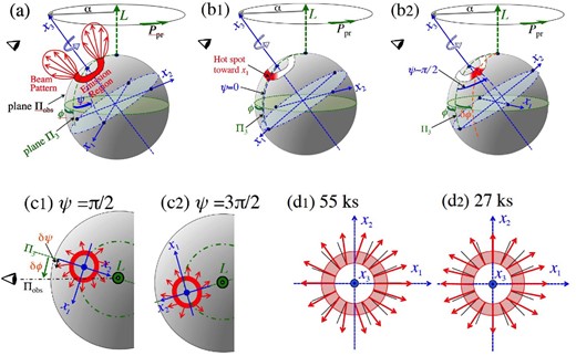
Toy model to explain the pulse-phase modulation phenomenon of 4U 0142+61. (a) The assumed basic geometry of an axi-symmetric star, where |$\boldsymbol {L}$| is the angular-momentum vector fixed to the inertial frame, |$(\skew4\hat{x}_1,\skew4\hat{x}_2,\skew4\hat{x}_3)$| denote the principal axes of the body, Πobs (= the plane of the sheet) is the plane containing |$\boldsymbol {L}$| and the observer’s line-of-sight, Π3 is that defined by |$\boldsymbol {L}$| and |$\skew4\hat{x}_3$|, α is the wobbling angle, φ is the pulse phase, and ψ is the slip phase; see text for details. A ring-shaped emission region in red is assumed, together with a sketch of the beaming pattern. (b1) The case wherein the ring-shaped region has a hot spot at an azimuth of |$+\skew4\hat{x}_1$|, and the slip phase is ψ = 0. (b2) The same as panel (b1) but for ψ ∼ π/2. (c1) A top view on to |$\boldsymbol {L}$|, illustrating the case when the beaming direction is tilted along the ring just one cycle per 2π, and the slip phase is ψ ∼ π/2. (c2) The same as panel (c1), but for ψ ∼ 3π/2. (d1) The same beaming patterns as in panels (c1) and (c2), but drawn on a plane perpendicular to |$\skew4\hat{x}_3$|, where arrows indicate the projected beaming direction. The tilt changes one cycle over the 2π azimuth. The black ticks indicate the radial directions. (d2) The same as panel (d1), but the tilt angle changes two cycles. (Color online)
The angle of |$\skew4\hat{x}_1$| measured from Π3 shall be denoted as ψ. It is identical to 2πt/T in equation (7), with ψ0 just its initial value, and changes with the period T to specify slip phase. Assuming a prolate deformation (ε > 0; Paper I), the precession is prograde, so ψ increases in the same direction as φ, though some 104 times more slowly [equation (3)].
In a double-folding map like figure 6a, we can identify φ and ψ with 2πk/K (abscissa) and 2πj/J (ordinate), respectively, except a constant initial value. In addition, (φ, α, ψ) provide the three Euler angles to describe the NS’s attitude with respect to the inertial frame.
4.5.2 Emission geometry for the Suzaku results
In figure 13a, a toy model for the hard X-ray emission is also illustrated. There, the HXC is thought to be emitted from a ring-like source (shown in red), located at one of the two magnetic poles. The emission is assumed to be moderately collimated towards the direction normal to the local NS surface. We do not consider the emission from the other pole, because its contribution, probably in the form of the secondary pulse peak, is weak and free from the phase modulation effect (subsection 3.5). For the same reason, neither do we require that the third symmetry breaking should take place simultaneously in both poles.
The source brightness is first assumed, as in panel (a), to be constant along the ring azimuth, and hence the emission is symmetric around |$\hat{x}_3$|. Then, the observed data are evidently insensitive to ψ, and the pulsation will be exactly periodic at Ppr. Because the source is extended and the beaming is assumed to be not too strong, the pulse profile is expected to have a single broad peak at φ = 0, if the line-of-sight makes a moderate inclination to |$\boldsymbol {L}$|. (If the inclination is more pole-on, the pulse peak could split into two.) A double-folding map such as figure 6a will be characterized by a straight vertical ridge. This case is considered to explain the SXC pulses, which are free from phase modulation.
Next, assume that the source brightness is non-uniform along the ring, and is concentrated, as in panels (b1) and (b2), to form a hot spot towards the |$+\hat{x}_1$| direction. The pulse profile will become sharper than in panel (a), because the source size has effectively diminished. At the slip phase ψ = 0 [panel (b1)], the pulse peak will still reach us at φ = 0 with no phase shifts, because the hot spot then lies on Π3. In contrast, at the slip phases ψ ∼ π/2 when the configuration is as in panel (b2), the hot spot will cross Πobs slightly before Π3 coincides with Πobs. The pulse peak will hence arrive by a small amount (δφ) earlier than the expected (φ = 0). The pulse-phase shift will return to 0 at ψ ∼ π, and at ψ ∼ 3π/2, the peak will be delayed by −δφ. Thus, the pulse phase becomes dependent on ψ.
Supposing that α takes an intermediate value (e.g., ∼45°), and the assumed ring has a relatively small half-cone angle β (say, β ∼ 10°), the amplitude of pulse-phase modulation would be at most A/T = δφ/2π ≲ β/360° ∼ 0.03. However, A can become larger if the direction of the maximum emissivity, or beaming direction, is titled outwards from the local normal to the NS surface, so that it points away from |$\hat{x}_3$|. This is the configuration considered in Paper I, to explain the sinusoidal pulse-phase modulation with a relatively large amplitude of A/T ∼ 0.08 as measured with the Suzaku HXD in 2009.
Strictly speaking, the pulse intensity will also be modulated, to become maximum and minimum at ψ = 0 and ψ = π, respectively, although this effect was not clear with the Suzaku data due to the limited statistics (subsection 4.4). A search for this effect is one of our future tasks (subsection 4.7).
4.5.3 Emission geometry for the NuSTAR results
So far, non-uniform brightness distributions of the ring-shaped emission source, possibly augmented by a tilt in the beaming direction, were invoked to break the symmetry around |$\hat{x}_3$|, or equivalently, in ψ. Although this has been successful for the 2009 and 2013 Suzaku data, it may not afford an adequate explanation for the NuSTAR results. In fact, trying to explain the emergence of Zp27, the ring might be assumed to have two symmetric hot spots, at azimuths towards |$\hat{x}_1$| and |$-\hat{x}_1$|. Then, on a double-folding map, the two hotspots would each wiggle one cycle per T, crossing a common vertical line in an anti-symmetric way. This would modulate, twice per T, the width of the vertical ridge in the plot, but would not produce such periodic displacements of the brightness centroid, twice per cycle, as seen in figure 8a.
As an alternative idea to break the symmetry around |$\hat{x}_3$|, we may assume that the brightness is rather uniform, but the beaming direction is tilted from the local normal, this time azimuthally in the ±ψ direction, and this tilt angle depends on ψ (Paper I). As in panels (c1) and (c2), let us assume that the beaming direction is most forward-tilted by δψ > 0 at the azimuth |$-\hat{x}_2$|, and most backward-tilted by −δψ at |$+\hat{x}_2$|, so that the overall emission axis (usually parallel to |$\hat{x}_3$|) is inclined towards |$\hat{x}_1$|. Then, at a slip phase of ψ ∼ π/2 [panel (c1)] and ψ ∼ 3π/2 [panel (c2)], the pulse peak will reach the observer slightly before and after the prediction (φ = 0), respectively. The amount of this pulse-phase shift is expressed as δφ = fδψ, were f is a form factor (0 < f < 1) which depends on the beaming strength and approaches unity if the beaming is very strong. Since we expect A/P ∼ δφ/2π = fδψ/2π, a tilt by δψ ∼ 30° and a moderate value of f ∼ 0.2 would be adequate to explain the observed amplitude of A/P ∼ 0.02. This condition is thought to explain Zp55 of the present NuSTAR data.
The above case assumed that the tilt angle of the beaming direction changes by one cycle along the ring azimuth. This condition is reproduced in panel (d1), in the form of projection on to the plane perpendicular to |$\hat{x}_3$|. In contrast, panel (d2) depicts the case wherein the beam tilt angle changes twice over the 2π azimuth, so that the emission is stronger in the |$\hat{x}_1$|–|$\hat{x}_3$| plane than in the |$\hat{x}_2$|–|$\hat{x}_3$| plane. Then, the pulse-phase shift is expected to have a period of T/2 instead of T, in a qualitative agreement with the appearance of Zp27. The relative azimuths of panel (d1) and panel (d2) has actually been selected to meet the observed relation between ψ0 ∼ 60° for Zp55 and ψ0 ∼ 300° for Zp27 (table 1). Finally, a configuration like panel (d2) may also bring about fine structures in the pulse profile, and could explain the N-dependence of Zp27 (item 5 in subsection 4.1).
In summary, the assumed ring-shaped emission region model can explain, by invoking non-uniform brightness distributions and an outward tilt in the beaming direction, the relatively large values of A/P found with Suzaku in 2009 and 2013. The model can also explain, in terms of radiation-beam tilt in azimuthal directions, the NuSTAR (and possibly the 2007 Suzaku) results with the very small A/P ratio and the prominent Zp27 feature. These two modes of symmetry-breaking effects are likely to be taking place more or less simultaneously, because Zp27 was observed in the 2013 Suzaku data as well (figure 12b).
4.6 Comparison with 1E 1547−5408
To generalize the results from 4U 0142+61 to the knowledge of the magnetars as a class, comparison with 1E 1547−5408 is valuable, because a very similar hard X-ray pulse-phase modulation was detected at |$T=36.0^{+4.5}_{-2.6}\:$|ks with Suzaku from this fastest rotating magnetar (Paper II). Here we briefly update our discussion made in Paper II.
The two magnetars both exhibit pulse-phase modulations, with two important similarities. One is that the asphericity implied by equation (2) is similar, ε = 1.6 × 10⁻⁴ for 4U 0142+61 and ε = 0.6 × 10⁻⁴ for 1E 1547−5408, both assuming cos α ≈ 1. The other is that the effect is seen only in the HXC, and is absent (or much weaker) from the SXC. In contrast to these similarities, the two objects differ considerably in their values of A/P, as 1E 1547−5408 has A/P ∼ 0.25 (reaching a quarter pulse phase), which is much larger than those of 4U 0142+6, A/P ≲ 0.08. Thus, the relative amplitude A/P is likely to exhibit a variety of behavior, among different magnetars, as well as among different observations of the same objects.
In Paper II, the 36 ks phase modulation of 1E 1547−5408 was explained by invoking a fan-beam like emission pattern. This is because its pulse profile was double-peaked, and the phase modulation appeared primarily as periodic intensity interchanges between the two pulse peaks. However, this concept is not much different from the ring-shaped emission region assumed in figure 13, because such a ring-shaped region is expected to have a conical emission pattern, which will become a fan-beam configuration as the outward tilt of the beaming direct gets larger. This suggests a possibility of constructing a more generalized model that can explain the behavior of the two sources, in terms of differences in the model parameters including α, the viewing inclination, the ring half-cone angle β, and the outward/azimuthal tilts of the beaming directions.
4.7 Future works
Before concluding the paper, we should touch on several future works to be performed. The most obvious one is a more systematic re-analysis of the three Suzaku data sets (2007, 2009, and 2013) of 4U 0142+61, plus another shorter one (gross 80 ks) acquired in 2011 September as a follow-up to a transient brightening of this magnetar.
Although the toy model of figure 13 appears to explain the Suzaku and NuSTAR observations of 4U 0142+61 in a consistent manner, it is still rather primitive. We clearly need to make it more quantitative, via numerical modeling of the geometry and beaming properties of the assumed emission region, to examine whether the model can actually explain the pulse-phase modulation in the data, as well as the observed pulse profiles and possible ψ-dependent intensity changes. Furthermore, as mentioned in subsection 4.6, we need to generalize the model so that it can account for not only the four observations of 4U 0142+61, but also the behavior of 1E 1547−5408. Through such a modeling, we will be able to obtain some estimates on α of the two objects, which remain at present only coarsely constrained to be neither ≈0 nor ≈90° (Paper II). These are also left for our future studies.
An even more important future work is to find physical grounds to the toy model of figure 13, and investigate mechanisms which can explain the switch between Zp55 and Zp27 (item 4 in subsection 4.1). Similarly, the transition between the large-amplitude modulation seen in 2009/2013 and the small-amplitude cases as in 2007/2014 need to be accounted for. Here, we only mention that the HXC could be produced via a quantum-electro-dynamical process called photon splitting (e.g., Enoto et al. 2010), where some input gamma-ray photons keep splitting towards softer photons, as they propagate along the MF lines that are stronger than the critical field value of |$B_{\rm c} \equiv m_{\rm e}^2 c^2 /e \hbar = 4.4 \times 10^{9} T = 4.4 \times 10^{13}\:$|G; here, me, c, e, and ℏ are the electron mass, the light velocity, the elementary charge, and the Dirac constant, respectively. Then, the phenomena considered in figure 13 could emerge as a result of incessant changes in the magnetic field configuration near the magnetic poles, where multi-pole structure may be involved. Conversely, further studies of the present phenomenon will give valuable clues to the emission mechanism of the HCX.
Finally, we need to increase the number of magnetars that exhibit the same phenomenon, in addition to 4U 0142+61 and 1E 1547−5408. This will allow us to examine whether magnetars are all axially deformed, and if so, how their ε (and hence the toroidal MF strengths) depends on their parameters including the age, the pulse period, and the dipole MF strengths. At the same time, a comparison of the same object at different intensity levels would be of great value, because 4U 0142+61 remained at a relatively similar intensity level through the four observations.
5 Conclusion
As confirmed consistently with the 2009 and 2013 Suzaku data sets, and those from NuSTAR obtained in 2014, the 8.69 s hard X-ray pulsation of 4U 0142+61 is phase modulated at a period of 55 ks, whereas its soft X-ray pulsation is not.
The modulation amplitude varies by a factor of 4–7 on time scales of months to years, and sometimes the second harmonic of the 55 ks periodicity appears at about half that period.
The scenario proposed in Paper I has been reconfirmed: the pulse-phase modulation is interpreted as caused by free precession of the neutron star, which is deformed to ε ∼ 1.6 × 10⁻⁴, possibly due to internal magnetic fields reaching ∼1016 G.
Major properties of the pulse-phase modulation are understood if the hard X-ray source has a certain geometry, and exhibits a variable degree of asymmetry in its position and/or beaming direction around the star’s axis.
The similarity between 4U 0142+61 and 1E 1547.0−5408, discussed in Paper II, remains valid. Namely, both objects are likely to be axially deformed to ε ∼ 10−4, and undergo free precession.
Acknowledgments
The authors thank Toshio Nakano and Yoshihiro Furuta for their help in data analysis and participation in discussion. This work was supported partially by the Ministry of Education, Culture, Sports, Science and Technology Grant-in-Aid for Scientific Research (C), Grant No. 18K03694.
References
