


Abstract
The Subaru Strategic Program (SSP) is an ambitious multi-band survey using the Hyper Suprime-Cam (HSC) on the Subaru telescope. The Wide layer of the SSP is both wide and deep, reaching a detection limit of i ∼ 26.0 mag. At these depths, it is challenging to achieve accurate, unbiased, and consistent photometry across all five bands. The HSC data are reduced using a pipeline that builds on the prototype pipeline for the Large Synoptic Survey Telescope. We have developed a Python-based, flexible framework to inject synthetic galaxies into real HSC images, called SynPipe. Here we explain the design and implementation of SynPipe and generate a sample of synthetic galaxies to examine the photometric performance of the HSC pipeline. For stars, we achieve 1% photometric precision at i ∼ 19.0 mag and 6% precision at i ∼ 25.0 in the i band (corresponding to statistical scatters of ∼0.01 and ∼0.06 mag respectively). For synthetic galaxies with single-Sérsic profiles, forced CModel photometry achieves 13% photometric precision at i ∼ 20.0 mag and 18% precision at i ∼ 25.0 in the i band (corresponding to statistical scatters of ∼0.15 and ∼0.22 mag respectively). We show that both forced point spread function and CModel photometry yield unbiased color estimates that are robust to seeing conditions. We identify several caveats that apply to the version of HSC pipeline used for the first public HSC data release (DR1) that need to be taking into consideration. First, the degree to which an object is blended with other objects impacts the overall photometric performance. This is especially true for point sources. Highly blended objects tend to have larger photometric uncertainties, systematically underestimated fluxes, and slightly biased colors. Secondly, >20% of stars at 22.5 < i < 25.0 mag can be misclassified as extended objects. Thirdly, the current CModel algorithm tends to strongly underestimate the half-light radius and ellipticity of galaxy with i > 21.5 mag.
1 Introduction
Wide-field, multi-band imaging surveys have stepped on to the central stage of modern astrophysics and cosmology over the past decade. These efforts will soon be replaced with even more ambitious programs such as the Large Synoptic Survey Telescope (LSST),1 the Wide-Field Infrared Survey Telescope (WFIRST: Dressler et al. 2012; Spergel et al. 2015),2 and the Euclid project (Laureijs et al. 2012).3 Among many ongoing efforts, the Subaru Strategic Program (SSP: Aihara et al. 2018b),4 which uses the Hyper Suprime-Cam (HSC: Miyazaki et al. 2012) on the prime focus of the Subaru telescope, is the most efficient in terms of etendue.5 Surveys such as HSC, and others to follow, will provide stringent constraints on the cosmological model, characterize the evolution of galaxies, map out the stellar structure of our Milky Way, and are poised to discover a large number of interesting transient objects.
Before we can tackle outstanding scientific questions, we must first learn how to handle the large amounts of data generated by these projects while satisfying strict requirements for high-quality image processing with accurate measurement for the magnitudes and shapes of stars and galaxies.6 Data handling becomes increasingly challenging in the age of modern imaging surveys as we aim to characterize and account for subtle effects related to charge-coupled devices (CCDs). Cameras are made up of multiple CCDs, each with slightly different characteristics, and have large fields-of-view (FoVs) over focal planes that are not perfectly flat. During observations, the seeing and background conditions display spatial and temporal variations across the FoV. The full-depletion, thick CCDs selected for HSC enable long exposure times and have excellent red-sensitivity, but they also suffer from the so-called “brighter-fatter” effect (Antilogus et al. 2014; Guyonnet et al. 2015), which means that brighter stars have larger point spread functions (PSFs) than fainter stars. These variations and effects make accurate astrometric and photometric calibration, background subtraction, and PSF modeling intrinsically difficult (e.g., Schlafly et al. 2012). Furthermore, as surveys reach to increasingly deeper detection limits (e.g., the SSP Wide layer reaches a 5σ point source detection limit of ∼26.4 mag in the i band), the number of objects per unit area increases. Hence, deep surveys become more sensitive and subject to the effects of blending. The challenge of modern imaging surveys calls for photometric measurement methods that are more powerful and precise than those used in previous, shallower surveys.
These challenges are not merely technical details; their resolution is crucial to achieving key scientific goals. For instance, weak gravitational lensing (WL: Kaiser & Squires 1993; Bartelmann & Schneider 2001) is a powerful tool for measuring the large-scale distribution of dark matter. However, WL measurements critically depend on our ability to measure the shape and photometric redshifts of background galaxies with high precision. Photometric redshifts (e.g., Benítez 2000; Bolzonella et al. 2000; Ilbert et al. 2009) are fundamentally important for studying the evolution of galaxies, and the “drop-out” method is critical for selecting high-redshift galaxies (e.g., Steidel et al. 1996). However, both of those methods rely on the availability of accurate multi-band photometric measurements. With increasingly large surveys, and with more stringent requirements on data quality, quality control also becomes a pressing issue.
In this paper, we present a Python-based software package called SynPipe that injects synthetic objects into HSC images and which interfaces with the HSC data reduction pipeline (hscPipe). Among other applications, SynPipe can be used to perform quality control and to characterize the performance and limitations of hscPipe. Several tools with similar goals have been developed (e.g., Chang et al. 2015; Suchyta et al. 2016) for the Dark Energy Survey (DES: The Dark Energy Survey Collaboration 2005).
In section 2, we briefly introduce the HSC survey and the current status of data reduction. In section 3, we explain SynPipe design and implementation. In section 4, we demonstrate SynPipe usage via straightforward tests, and we show the main results for the general photometric quality of synthetic stars and galaxies in section 5. We demonstrate other applications of SynPipe in section 6 and provide more discussions in section 7. We then summarize the results in section 8.
Throughout this work, all magnitudes are in the AB system (Oke 1974). Signal–to–noise ratio (S/N) is defined as the ratio between a flux measurement using a specific algorithm (e.g., PSF, CModel) and its corresponding flux uncertainty from hscPipe [Flux/σ(Flux)]. A 5σ detection is equivalent to a flux measurement with S/N = 5 using PSF photometry. The same definitions are adopted in other work using HSC-SSP data (e.g., Bosch et al. 2018; Aihara et al. 2018b). The code for SynPipe, along with documentation and examples, is made available on GitHub.7
2 Hyper Suprime-Cam Subaru strategic program (HSC Survey)
2.1 Status of the survey
Taking advantage of the new prime focus camera on the 8.2 m Subaru telescope, the ambitious HSC survey consists of three layers: Wide, Deep, and UltraDeep. The Wide layer will map a total of ∼1400 deg2 of sky in five broad bands (grizy: Kawanomoto et al. 2017). The Deep (four separated fields; ∼27 deg2) and UltraDeep (two separated fields; ∼3.5 deg2) layers use a few additional narrow-band filters and employ a slightly different surveying strategy. Aihara et al. (2018a) describes the HSC survey in more detail, and identifies the HSC collaborators.
The HSC camera (Miyazaki et al. 2012) is made up of 124 full-depletion thick CCDs: 112 for science and another 12 for guiding and focusing. The camera has a circular FoV with a 1|${^{\circ}_{.}}$|5 diameter. Each CCD contains 2048 × 4096 pixels and the sizes of pixels are 0|${^{\prime\prime}_{.}}$|168. For more details about the HSC camera, please see Miyazaki et al. (2018).
In 2017 February, the HSC collaboration released the first 1.7 years of data to the public (DR1: Aihara et al. 2018b).8 For our work, we focused on data from the Wide layer as they relate to key scientific goals of the HSC survey, which include weak lensing cosmology, galaxy evolution, and studies of galaxy clusters. The Wide layer data in DR1 correspond to ∼108 deg2 spread over six fields (XMM-LSS, GAMA09H, WIDE12H, GAMA15H, HECTOMAP, and VVDS).9 Except for the HECTOMAP field, the regions are all close to the equator. In the Wide layer, the g and r bands have 10 min exposures broken into four dithers. The i, z, and y bands have 20 min exposures broken into six dithers. The survey prioritizes the observations so that the i band has the best seeing conditions to improve galaxy shape measurements for weak lensing science. The i band data in the Wide layer reach a 5σ point source limiting magnitude of i ∼ 26.4 mag and have a median seeing with FWHM ∼ 0|${^{\prime\prime}_{.}}$|6 in the i band. Aihara et al. (2018b) provides details on the first data release and data status.
2.2 The HSC data reduction pipeline
The HSC data are reduced using a pipeline that builds on the prototype pipeline being designed for the LSST’s Data Management system (Ivezic et al. 2008; Axelrod et al. 2010; Jurić et al. 2015) and is described in Bosch et al. (2018). To enhance the flexibility and modularity of the pipeline, hscPipe is written using a combination of C++ and Python. All computationally intensive pixel-level operations are performed in C++, while high-level connections between routines and the user interface are written in Python. DR1 data are reduced by hscPipe v4.0.5. Because SynPipe is intrinsically connected to the complex data reduction processes in hscPipe, we briefly introduce the main steps below, along with a few key HSC/LSST terms.
Single-visitprocessing: Each individual exposure is called a visit and is assigned an even integer. After initial data screening (considering the background level, seeing, and transparency; Furusawa et al. 2018), hscPipe subtracts overscan, bias, and dark frames, and performs flatfielding to the single CCD images. During this step, hscPipe also generates variance and mask images, subtracts the background, and provides initial astrometric and photometric calibrations. The photometric calibration is based on data from the Panoramic Survey Telescope and Rapid Response System (Pan-STARRS) 1 imaging survey (Schlafly et al. 2012; Tonry et al. 2012; Magnier et al. 2013). SynPipe uses the spatially varying PSF models, photometric zeropoints, and the World Coordinate System (WCS: Greisen & Calabretta 2002; Calabretta & Greisen 2002) corrected for optical distortion provided by hscPipe.
Multi-visitprocessing: After single-visit processing, hscPipe warps and mosaics the reduced CCD images into much deeper coadd images while improving the astrometric and photometric calibrations via processes similar to the über-calibration in the Sloan Digital Sky Survey (SDSS) (Padmanabhan et al. 2008). SynPipe will use these improved calibrations. hscPipe organizes these coadd images into equiareal rectangular regions, or tracts, which are predefined as iso-latitude tessellations. One tract covers approximately 1|${^{\circ}_{.}}$|7 × 1|${^{\circ}_{.}}$|7 and adjacent tracts overlap each other by ∼1΄. Each tract is further divided into 9 × 9 Patches. A Patch is a 4200 × 4200 pixel rectangular region, and adjacent Patches overlap each other by 100 pixels.
Multi-band measurements: To achieve consistent photometry across all filters, hscPipe first detects and deblends objects on coadd images in each band independently (the unforced measurements). The collection of above-threshold pixels for each object is referred to as a footprint. hscPipe merges the footprints and flux peaks in the different bands and then selects a reference band for each object based on its S/N in each band (usually this corresponds to the i band). Centroids, shapes, and other non-amplitude parameters are then fixed to the values from the reference band. hscPipe then performs forced photometry using these fixed quantities. The goal of the forced photometry step is to generate accurate colors.
HSC photometry: The multi-band catalogs generated by hscPipe contain various types of photometric measurements (see Aihara et al. 2018b for details). Here, we focus on characterizing the the forced psf and CModel photometry. Both the PSF and CModel photometry algorithms take the PSF convolution effect into account, and hence can provide consistent forced photometry across all bands and maximize S/N. Although their accuracy depends on the accuracy of the PSF model and choice of a model, they still provide the most useful flux information for stars and galaxies, especially for objects with low-S/N. Please see section 4 and appendix 2 of Bosch et al. (2018) for detailed descriptions of these algorithms.
Details of the HSC PSF photometry can be found in sub-subsection 4.9.5 of Bosch et al. (2018). In short, hscPipe uses matched-filter method to derive PSF magnitude with the centroid fixed. The algorithm matches the image of a star with the PSF model multiplied by an amplitude. This amplitude parameter is estimated via the inner product of the image and PSF model after shifting the model to the centroid of the star, then divide by the effective area of the PSF model. It considers the per-pixel variance information when estimating the flux error. Flux uncertainty due to the uncertainty of centroid is ignored since it is subdominant even when the S/N is low.
Details about the HSC CModel photometry can be found in sub-subsection 4.9.9 and appendix 2 of Bosch et al. (2018). It is based on the algorithm used for the SDSS CModel magnitude (Lupton et al. 2001; Abazajian et al. 2004). It fits an object using elliptical models with an exponential profile and de Vaucouleurs profile with free amplitudes and shapes, then fits a linear combination of both models to the image while only allowing the amplitude of each component to change. The last step provides the CModel flux and flux error used in this work. This CModel flux can be roughly seen as the linear interpolation between exponential and de Vaucouleurs models. Although these models are often not the most appropriate models for real galaxies, this method is shown to be robust and efficient, especially for poorly–resolved and/or low S/N galaxies. Star–galaxy classification is also now performed based on the difference between psf and CModel magnitudes.
DR1 data quality has been vetted in Aihara et al. (2018b) by cross-checking with the Pan-STARRS 1 imaging survey to examine the behavior of the stellar sequence. Generally speaking, the PSF photometry is accurate at the 1%–2% level for bright stars, and the astrometry is accurate to ∼10 and 40 mas internally and externally.
3 SynPipe overview
3.1 Design
hscPipe is a complex data reduction pipeline that still faces many challenges and is under active development. Unlike other publicly available photometric pipelines that focus on the low-level reduction processes such as detrending and calibrating the images, hscPipe involves high-level reduction processes that produce not only deep coadd images but also a series of science-ready catalogs. To perform tests of the data products that result from hscPipe, SynPipe is designed to satisfy a few basic standards:
Realistic images: Instead of using a fully generative approach to simulate full HSC-like images from the ground up (e.g., Chang et al. 2015), SynPipe injects synthetic objects into real HSC images so that all the realistic features of the real data (e.g., blended objects; proximity to bright objects, bleeding trails, other optical artifacts) can be included in the test. The impact of these features can be important for studies that care about completeness and the selection function. In SynPipe, point sources are simulated using the HSC PSF model, and a realistic galaxy model is created by the modular galaxy image simulation toolkit, GALSIM (Rowe et al. 2015).10
Authentic data processing: To follow the data reduction process as realistically as possible, we choose to start from the single-visit images instead of directly putting synthetic objects on the final coadd images (e.g., Suchyta et al. 2016). Through this approach, subtle effects like seeing differences among visits and small errors in astrometric calibration can be taken into account. Every synthetic object will experience all the steps we would use for a real object: detection, deblending, stacking, and measurement. This can be important for challenging tasks like WL measurements or the detection of high-z galaxies. The downside of this choice is that it slows down the overall run-time because we need to inject synthetic objects into all the visits that contribute to a tract.
Flexible capabilities: SynPipe is designed to be flexible enough to be useful for HSC users with a range of scientific goals. We provide default catalogs to generate samples of synthetic stars and galaxies with realistic magnitudes and color distributions along with tools to help the user work on HSC DR1 data. However, the users can also supply their own input catalogs best suited for their applications. SynPipe is already being used in a wide range of scientific topics (see section 8 for details).
SynPipe works as a special user interface to hscPipe. It will keep developing along with the hscPipe (and LSSTpipe in the future). Since both hscPipe and GALSIM use Python as their high-level language, we also choose to use Python for SynPipe to make the frequent interactions among them easy and straightforward. Most of the computationally expensive tasks are handled by low-level algorithms in hscPipe and GALSIM that are written in C++. As a result, the fact that high-level routines are written in Python does not affect the overall efficiency of SynPipe.
3.2 SynPipe Implementation
In this section, we describe the SynPipe test implementation illustrated in figure 1.
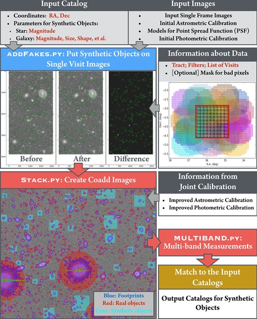
Illustration of the workflow of SynPipe. Gray boxes indicate required inputs at different stages. The blue box identifies the addFakes.py step, when SynPipe injects synthetic objects into single-frame images. Below the blue box, we show an HSC image before and after the insertion of synthetic galaxies. The positions of synthetic objects are highlighted with green circles. Red boxes depict the image coadding and multi-band measurement steps using stack.py and multiBand.py. At the bottom left, we show a coadd image which contains synthetic galaxies. On the right-hand side, we show the spatial relation between tracts, patches, and visits. The red colored box corresponds to one tract which has an area of about 1.5 deg2. Large colored circles are visits (also commonly known as “pointings”) with small rectangles representing CCDs. patches are represented by black dashed lines. One tract typically contains 81 patches. (Color online)
3.2.1 Preparation
To create a catalog of synthetic objects, the user first needs to select which HSC data and which input synthetic galaxy catalog to use.
Information about the data. This corresponds to the location of HSC images and a list of visits to be used. SynPipe can also help the user identify all the visits that contribute to one tract in any given band. SynPipe also provides tools to create an optional bad-pixel mask (e.g., bright object, bleeding trails) for a specific tract so that the user can avoid putting synthetic objects on problematic regions.
Input catalog. This is a catalog in FITS (Flexible Image Transport System) format that contains the coordinates, magnitudes, and model parameters of synthetic objects. The positions of synthetic galaxies can be specified via the input catalog; they can be distributed randomly over a given region, or on an evenly-spaced grid (the grid option is useful in that it avoids blends between synthetic objects, e.g., see R. Murata et al. in preparation).
Synthetic objects can be one of the following:
Point source: SynPipe simply uses the PSF model from hscPipe as the model for a point source (stars and/or quasi-stellar objects). hscPipe uses a special version of PSFEx (Bertin 2011, 2013) to characterize PSF as a function of position and the PSF model can be reconstructed for any location on the image. To inject point sources, the user only needs to specify a catalog of coordinates and magnitudes.
Sérsicmodels: SynPipe uses GALSIM v1.4 (Rowe et al. 2015) to simulate galaxies. GALSIM is an image simulation tool that was designed for the GRavitational lEnsing Accuracy Testing 3 (GREAT3) challenge (Mandelbaum et al. 2014). Currently, SynPipe allows synthetic galaxies to be modeled by a single or a double Sérsic (1963) profile.11 The Sérsic profile is flexible enough to describe the overall flux distributions of galaxies near and far, both early-type or late-type. A double-Sérsic model can simulate a galaxy with even more realistic structural details (e.g., bulge + disk). For each Sérsic component, the user needs to provide the magnitude, effective radius (Re, in units of arcseconds), Sérsic index (nSer), axis ratio (b/a), and position angle (PA). External shear can also be applied to a synthetic galaxy (g1 and g2, see Rowe et al. 2015 for more details). To generate a synthetic image of a Sérsic or double-Sérsic galaxy model with a high level of numerical accuracy, the pixel integration (especially for central pixels) and image rendering process must be carefully handled. Details about these can be found in sections 5 and 6 of Rowe et al. (2015), with validation of numerical accuracy also shown in that paper.
Galaxies from the GREAT3 challenge: SynPipe also allows users to choose from parametric models or real high-resolution galaxy images used in the GREAT3 WL challenge. Real galaxy images are drawn from the HST/ACS F814W (I band) images of galaxies in the COSMOS field (e.g., Scoville et al. 2007; Leauthaud et al. 2007). Instead of using real galaxy images, the users may also use models of COSMOS galaxies to IAuto ≤ 25.2 mag via a method developed by Lackner and Gunn (2012). Parametric models of COSMOS galaxies include a single-Sérsic and the Sérsic bulge + Exponential disk model. The parameter values for these models are stored in the GalSim.COSMOSCatalog() catalog. To access them, the user can provide the ID number of COSMOS galaxies in the input catalog, or can simply opt to let SynPipe randomly select galaxies from the COSMOS input catalog.
3.2.2 Injection of synthetic objects into single-visit images
With the input catalog and test data information in hand, SynPipe injects synthetic objects into single-exposure images (step addFakes.py; see the middle panel of figure 1). SynPipe goes through individual CCD images that belong to each visit and decides which synthetic objects from the input catalog need to be injected. SynPipe uses the initial astrometric calibration of each single visit to convert the input coordinates into locations on the CCD image. For each synthetic object, SynPipe uses the reconstructed PSF for each exposure. The photometric zeropoint from the single-visit calibration is used to convert input magnitudes of synthetic objects into fluxes.
With the help of the GALSIM module, SynPipe simulates the images of synthetic objects.
– For point sources, SynPipe generates a rectangular cutout image of the PSF model with appropriate size and correct total flux.
– For galaxies described by single- or double-Sérsic models, SynPipe passes the input Sérsic index and effective radius to the GALSIM.Sersic function to create a Sérsic component. After stretching and rotating the galaxy to the expected axis ratio and position angle via the shear and rotate methods, SynPipe assigns the correct flux to this component.
– For a double-Sérsic model, SynPipe uses the GALSIM.Add method to combine two Sérsic components.
– For parametric models from the GREAT3 catalog, SynPipe uses the COSMOSCatalog.makeGalaxy method to generate models.
– For galaxies using any parametric model, we also generate rectangular cutout images. The model image can be truncated at N × Re to reduce the size of the cutout and speed up the injection process. In this work, we truncate all Sérsic models at 10 × Re. The results presented here are not sensitive to this choice.
– To inject real HST galaxy images, SynPipe calls the GALSIM.RealGalaxy method.
If necessary, an additional shear (g1 and g2) can be applied to the model at this point. Then, SynPipe passes the reconstructed PSF image into a GALSIMInterpolatedImage object and convolves it with the galaxy model using GALSIM.Convolve. After this, SynPipe uses the GALSIM.drawImage method to render the image of the simulated galaxy. A component with a high Sérsic index (nSer > 4) often requires a large image size to cover all of its flux, so SynPipe allows the user to truncate the model at a given radius (N × Re). SynPipe will also give warning information when a component with nSer > 6 is encountered because it takes much longer to achieve accurate PSF convolution in such a model; and the result is, therefore, not a realistic galaxy model.
After SynPipe creates the image of the simulated galaxy, it then shifts the image according to its location on the CCD on a pixel-by-pixel basis; SynPipe also crops the images when necessary. When that task is complete, SynPipe adds appropriate Poisson noise to the image based on the pixels it covers and the calibration information of the detector, and creates a variance image that reflects the influence of the synthetic object. Since each HSC CCD consists of four amplifiers, each with different characteristics, SynPipe carefully creates a corresponding gain map to provide accurate noise level. The added noise only accounts for the additional flux in the synthetic object, and will thus be subdominant compared to the noise already in the image for faint objects.
In the final step, SynPipe adds the noise-added image and the variance map to the original CCD data while also adding a new FAKE mask bit to the mask plane. The middle panel of figure 1 depicts the result of the addFakes.py step by showing an example CCD image before and after the synthetic objects are injected.
3.2.3 Stacking and multi-band measurements
The newly generated single-visit images have the same format and data structure as real HSC data. To perform stacking and measurements, SynPipe calls standard hscPipe routines.
The stack.py step takes the improved astrometric and photometric calibrations for each visit from the original reduction and creates coadd images that contain synthetic objects. The multiBand.py step then processes these coadd images and provides standard multi-band measurements in FITS catalogs that are grouped by Patch ID.
Using the infrastructure provided by hscPipe, the user can easily perform these steps in parallel. For coadd images that include the same number of single-visit data, the overall efficiency of SynPipe is similar to the real data reduction process under the same computational conditions (e.g., same number of cores). The stack.py and multiBand.py steps take similar amounts of time. The single-visit process is replaced with the injection of synthetic objects. The speed of this step depends on the total number of fake objects injected and the type of the synthetic object (e.g., a fake galaxy using a Sérsic model costs more time than a fake star). For tests with a reasonable density of fake objects per CCD (e.g., the tests in this work), the injection step takes slightly less time than the actual single-visit data processing. The data and catalog volumes are also similar to the original data reduction process.
The final step is to identify synthetic galaxies in the output catalogs. SynPipe can match the input catalog to the output catalog (this contains a mix of real and synthetic galaxies) using a matching radius specified by the user. Each unmatched object from the input catalog is also passed to the results catalog with a unique label. In the case of multiple matches, the user can choose between returning only the closest match or returning all objects within the matching radius (the nearest one is labeled as such).
3.3 Limitations and caveats
The limitations of the current SynPipe include the following:
Aihara et al. (2018b) points out that hscPipe tends to over-subtract the background around bright objects. Unfortunately, SynPipe now takes the original background subtraction on the single-visit image for granted; hence, it lacks the capability to test or help improve this problem.
SynPipe simply adopts the PSF measured by hscPipe and uses it as a model of point source and PSF convolution for a galaxy. Hence, it cannot be used to test how the uncertainty of the PSF modeling affects the photometry and shape measurements. This could be important for regions with exquisite seeing (e.g., FWHM ∼ 0|${^{\prime\prime}_{.}}$|4) that makes the PSF modeling difficult, and for accurate WL measurements (see Aihara et al. 2018b).
SynPipe works in a “unit” of visit for a single-exposure test, and uses a tract to test coadd images. In the case of tests that focus on specific regions that are much smaller than the size of a visit or a tract (e.g., quality of photometry around rich galaxy clusters), using SynPipe often leads to low efficiency.
4 Generation of synthetic dataset
We now describe the generation of the synthetic data set that we use to characterize the performance of hscPipe.
4.1 Data
We use tract = 9699 in the VVDS field (median FWHM = 0|${^{\prime\prime}_{.}}$|449 in the i band; in this paper referred to as goodSeeing) and tract = 8764 in the XMM-LSS field (median FWHM = 0|${^{\prime\prime}_{.}}$|700; badSeeing). tract = 9699 also has better seeing in both the r and z bands than the median conditions in those bands. The seeing conditions in the g and y bands are very similar for both tract = 9699 and tract = 8764. For both tracts, the coadd image in each band includes data from 20–40 visits.12 These two tract are selected because they are not at the edge of a field, do not contain any extremely bright (i < 12 mag) saturated stars, and are representative of both “good” and “bad” seeing conditions in the i band.13
4.2 Input models for stars and galaxies
We use a synthetic star sample built using data from the HST/ACS catalog of Leauthaud et al. (2007). We first select stars from the Leauthaud et al. (2007) catalog (this classification is reliable down to |$I_{\mathit {F814W}} \sim 25.2\:$|mag). We then match this sample against our HSC UltraDeep–COSMOS data (which reaches ∼27.2 mag in the i band). After applying basic quality cuts (see 1), this procedure provides us with five-band HSC PSF photometry for 14472 stars. To increase the sample size, we re-sample the five-band magnitude distributions using the astroML (VanderPlas et al. 2014) implementation of the extreme-deconvolution algorithm developed by Bovy, Hogg, and Roweis (2011) to generate 100000 synthetic stars.14 Figure 2 shows the magnitude and color distributions of real COSMOS stars compared to the resampled distributions in all five bands and in color–color space. It is worth noting that a SynPipe test using synthetic stars can also help determine the detection limit and point source completeness of the HSC data. However, both of those quantities depend on the seeing and background conditions, so their spatial variations must be considered. Doing so requires a higher density of synthetic objects than was used here, and is beyond the scope of this work. Please see subsections 5.6 and 5.7 of Aihara et al. (2018b) for an investigation of this topic for HSC-SSP DR1 using a different method.

Magnitude and color distributions of synthetic stars. Upper panel: five-band magnitude distributions of the COSMOS stars (filled histograms) and resampled stars (dashed lines). Lower panel: color–color distributions (left: g − r v.s. r − i; right: i − z v.s. z − y). Filled contours indicate COSMOS stars and open contours indicate resampled stars. (Color online)
For synthetic galaxies, we use single-Sérsic galaxy models of COSMOS galaxies with |$I_\mathit {F814W} \le 25.2\:$|mag. These are models from Lackner and Gunn (2012) applied to HST/ACS images and are included in GALSIM. Each model is described by a total of five parameters: magnitude, effective radius, Sérsic index, axis ratio, and position angle. It is worth noting that although the single-Sérsic profile is still an oversimplified model compared to the complexity in real galaxies, it is flexible enough to broadly describe the flux distributions of most galaxies, and test the CModel algorithm—which models the galaxy profile in a different way. In addition, the single-Sérsic model is sufficiently simple to serve as a straightforward diagnostic of potential systematic issues of the CModel algorithm. We exclude a tiny fraction (∼4%) of ill-behaved models that have a very high Sérsic index (nSer > 6.0) or a very low central surface brightness (μi < 24.0 mag arcsec−2). We further match this COSMOS sample with the HSC UltraDeep–COSMOS data. After removing objects with problematic photometry (see appendix 1 for details), we obtain a sample of 58210 synthetic galaxies with realistic five-band HSC CModel photometry. As shown in figure 3, the majority of these galaxies are faint (i < 24.0 mag) and barely resolved (Re < 1|${^{\prime\prime}_{.}}$|0). This sample is appropriate to test hscPipe’s general photometric behaviors, but the sample lacks relatively bright galaxies (i < 20.5 mag).
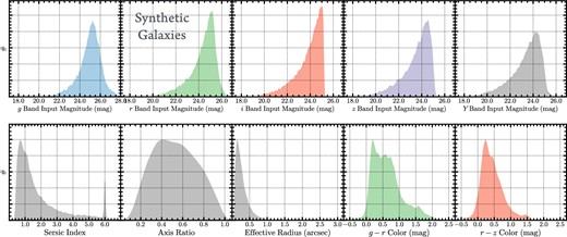
Upper panels show the five-band magnitude distributions of synthetic galaxies. Lower panels show the input parameters of the Sérsic model; from left to right are the input Sérsic index, axis ratio, effective radius in arcsec, the g − r and r − z colors). (Color online)
We spatially distribute synthetic stars and galaxies randomly in our two selected tracts. For stars, we use a number density of 1000 per CCD. For galaxies, we use a number density of 500 per CCD. Given the magnitude distributions of these objects, these numbers are high enough to ensure large sample of useful synthetic objects for the test, and will also not create unrealistic crowded images.
4.3 Generating SynPipe data
We use HSC DR1 data stored at the Kavli Institute for the Physics and Mathematics of the Universe (Kavli IPMU) for these tests. Using 108 cores, the addFakes.py step takes ∼1.5 hr per tract in each band for stars. The same process takes longer for galaxy tests (∼3.0 hr per tract in each band) because the GALSIM simulation is more time-consuming. The stack.py step and multiBand.py step together take ∼3.5 hr per tract.
We match the results with the input catalogs using a 2-pixel matching radius to generate output catalogs for forced and unforced photometry in each band. For our tests, we reject synthetic objects locate within 2 pixels of a real HSC object. These “ambiguously blended” (e.g., Dawson et al. 2016) objects are extreme blends in which multiple objects are detected as a single object, and are not useful for photometric tests.
The detailed log of our runs can be found at their web site.15 The user should be able to reproduce the results presented in this work using this information. It can also serve as a brief manual for generating SynPipe data.
5 Photometric performance results
Here we discuss hscPipe’s general performance, assessed mainly through forced PSF photometry (for stars) and (CModel) photometry (for galaxies). Although hscPipe does provide other options (e.g., aperture and Kron photometry), these two are the only options that consider the effects of the PSF in different bands and are consistent across all bands in terms of position and shape.
5.1 PSF photometry of stars
In hscPipe, the PSF magnitude is derived using a matched-filter method that depends on the best-fitting PSF model and uses third-order Lanczos interpolation to shift the PSF model. The error of the PSF magnitude from hscPipe only considers the per-pixel noise, and does not include centroid uncertainties. hscPipe also estimates aperture correction for PSF photometry. For more details please see Bosch et al. (2018).
We randomly inject ∼100000 stars into each tract in all five bands. Typically, there are ∼80000 stars with iPSF < 26.0 in one HSC tract. Approximately ∼3%–4% of the stars are located within 2 pixels of the centroids of real objects; we remove those stars from the sample to avoid confusion in the comparisons. For matched stars, we select the primary detections (detect.is-primary=True) that have good photometric quality (see appendix 1 for details). This gives us ∼83000 stars in each tract.
Next, we exclude stars that are misidentified by hscPipe as extended objects using the classification. extendedness parameter in each band. The fraction of misclassification is ∼10%–20%, and clearly depends on seeing conditions. For the same reason, the g band has the highest fraction of misclassification, while the i band is recommended for selecting point sources. The star–galaxy separation issue is discussed more in subsection 6.2.
In the following comparisons, we show the results from the goodSeeing and badSeeing tracts separately because it is important to understand how the seeing conditions affects photometric accuracy as well as to test whether hscPipe can deliver unbiased photometry under different seeing conditions.
Besides seeing, the degree to which an object is blended with other objects is another factor that influences photometric accuracy. To quantify the impact of blending effects, we use the “blendedness” parameter, b. This parameter describes how much any given object overlaps with neighboring objects (see appendix 2 and R. Murata et al. in preparation). We divide our sample according to the blendedness parameter. A value of b = 0 corresponds to isolated objects, whereas objects with b = 1 completely overlap with other objects. Here we use b > 0.05 to define highly blended stars (∼4%–9% are blended according to this criterion). The fraction of highly blended stars slightly increases in the badSeeingtract. The impact of blendedness will be discussed more in subsection 6.3.
5.1.1 Relationship between stellar magnitude and S/N
The S/N for PSF photometry is defined as |$\mathrm{Flux}_{\mathrm{PSF}}/ \mathrm{Flux\_Err}_{\mathrm{PSF}}$| in each band. The flux error here is estimated based on the per-pixel variance information that summarizes statistical uncertainties from various sources. However, the flux uncertainty due to the centroid uncertainty is not taken into account, as it should be subdominant even at low-S/N. As mentioned earlier, this definition of PSF S/N is adopted by Aihara et al. (2018b) and Bosch et al. (2018). Figure 4 shows the relationship between stellar magnitude and S/N in the g and i bands. This figure shows the expected S/N of stars as a function of magnitude in the Wide layer. The slopes and scatters of these relations are very similar to the ones using real stars on these two tracts.
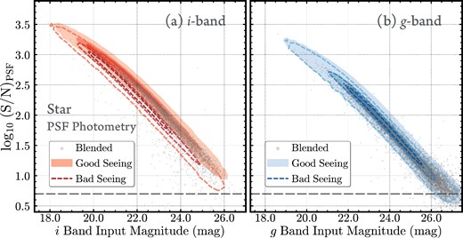
Relation between input magnitudes (left: i band; right: g band) of synthetic stars and the log (S/N) measured by hscPipe PSF photometry. Filled contours and open contours show the distributions for stars in the goodSeeing and badSeeing tracts, respectively. Highly blended stars with b > 0.05 are highlighted using scatter plots. The gray dashed line marks S/N = 5, which is the detection threshold used by hscPipe. Our 5σ point source detection limit is ∼26.5 mag in the i band, however we do not reach these magnitudes with our current synthetic stellar input catalog. (Color online)
Figure 4 shows that seeing conditions impact the S/N of point sources at fixed input magnitude. In the i band, the badSeeing (0|${^{\prime\prime}_{.}}$|70) tract shows systematically lower S/N than the goodSeeing (0|${^{\prime\prime}_{.}}$|45) tract. The S/N is similar for the two g-band tracts because they share similar seeing conditions.
At S/N = 5, HSC Wide can detect stars as faint as ∼26.5 mag in both g and i bands, which is consistent with the values found in Aihara et al. (2018b) for average seeing conditions. However, it is worth reminding HSC data users that the detection limit will exhibit spatial variations due to the seeing conditions. In addition, the image warping process introduces covariance between pixels into coadd images, and leads to slightly underestimated flux errors. Therefore, it is useful to compare the statistical results from our tests with the average PSF flux error at fixed input magnitude.
5.1.2 Precision and accuracy of PSF magnitudes
We now investigate the performance of the PSF photometry in each of the five bands independently. Figure 5 shows the difference between the input magnitude versus the hscPipe forced PSF magnitude (ΔmagPSF) as a function of input magnitude. We separate these stars into seven input magnitude bins. In each bin, we characterize the statistical precision of the PSF magnitude using the standard deviation of the distribution (σΔMag). Meanwhile, we characterize the statistical accuracy of the PSF magnitude via the mean magnitude difference in each bin (〈ΔMag〉). This also informs us whether the PSF photometry is biased at certain input magnitudes.
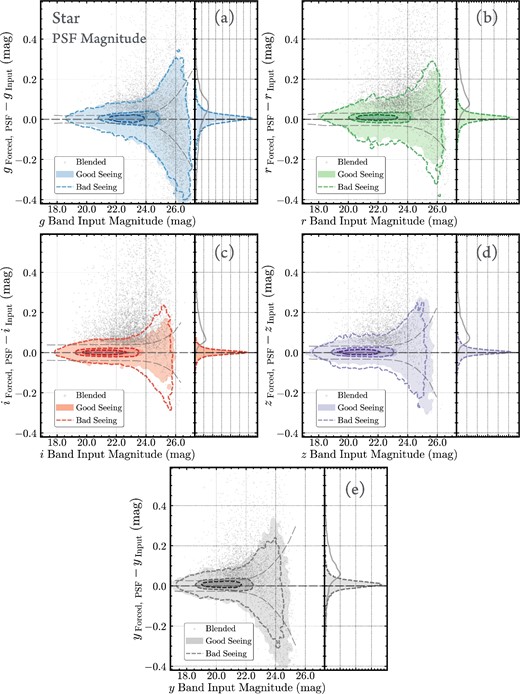
Accuracy of the hscpipe PSF photometry for synthetic stars measured by the difference between input and output forced PSF magnitudes. Plots (a), (b), (c), (d), and (e) show the results for the g, r, i, z, and y band, respectively. The left-hand panel in each plot shows the relation between input magnitude and magnitude difference. Filled and open contours are for the synthetic galaxies from goodSeeing and badSeeing tracts. Highly blended stars with b > 0.05 are highlighted using scattered points. The long-dashed lines mark zero magnitude difference, while the pairs of dashed lines outline the running-median of PSF magnitude errors (including the uncertainties in aperture correction). The right-hand panel in each plot shows the distributions of the magnitude differences for objects in goodSeeing (filled) and badSeeing (solid line) tracts. The dashed lines identify the distribution of highly blended objects. (Color online)
The overall performance of the hscPipe forced PSF magnitude is excellent. The median i-band PSF magnitude precision for the goodSeeing tract is ∼0.014 mag (∼1.3%) at iInput ∼ 19.0 mag. At iInput ∼ 24.0 mag, the precision of the PSF magnitude is at the ∼3% level (∼0.030 mag statistical scatter). At iInput ∼ 25.0 mag, the precision decreases to ∼6% with an average ∼0.062 mag difference.
The precision of PSF magnitude for the badSeeing tract shows similar performance at iInput < 23.5 mag. At fainter magnitudes, the precision slightly degrades. The badSeeing tract has ∼4% precision at iInput ∼ 24.0 mag and ∼11% precision at iInput ∼ 25.0 mag. Aihara et al. (2018b) evaluates the precision of PSF magnitude via external comparisons with the PS1, PV2, and SDSS data at i < 21 mag, and finds it at the 1%–2% level, which is consistent with our results. However, at fainter magnitudes, external comparisons become difficult due to the lack of imaging matched to HSC depths. The results from SynPipe hence provide useful evaluations of the precision of the HSC photometry down to our detection limit.16 In figure 5, we also compare the SynPipe test results with the median PSF magnitude error obtained by hscPipe in each bin after taking into account the uncertainty in the aperture correction (see sub-subsection 4.9.2 in Bosch et al. 2018)—see the pairs of grey long-dashed lines on each plot. We find that, for PSF photometry, the flux errors from hscPipe are very close to what we estimate using SynPipe once the aperture correction error is considered. Without the aperture correction error, it seems that hscPipe underestimates the statistical uncertainties of PSF magnitudes, most likely due to the correlated noise introduced during the image warping and stacking step.
Figure 5 also shows that the precision of the PSF photometry is not filter-dependent. The precision of forced PSF magnitudes in r and z is similar to the results for the i band. For the r band we find 1.5%–4.0% precision at rInput < 24.0 mag and ∼8% precision at rInput ∼ 25.0. For the z band we find 1.0%–5.0% precision at zInput < 24.0 mag and ∼10% precision down to zInput ∼ 25.0 mag).
The precision for the g and y bands becomes slightly worse at the very faint end. For the g band, the precision is 1.5%–7.0% at gInput < 24.0 mag and is ∼13% down to 25.0 mag. For the y band, we find 1.5%–5.0% precision at yInput < 23.0 mag and ∼12% down to 24.0 mag. These differences are however consistent with the differences in the seeing conditions between the filters
The PSF photometry for relatively isolated stars is accurate and unbiased in the i and z bands down to faint magnitudes. For the g, r, and y bands, we find mean ΔmagPSF that are close to the PSF flux errors estimated by hscPipe. hscPipe tends to underestimate the fluxes of stars in these bands by ∼0.01–0.02 mag at <24.0 mag. The exact cause of this offset is unclear but the levels of bias are quite small and not a major concern.
However, figure 5 also shows that blending has a strong impact on photometry. On average, hscPipe systematically underestimates the total fluxes of stars that are subject to blending effects by 0.05–0.10 mag at a fixed input magnitude. We see the same effect in all bands, and the impact of blendedness becomes increasingly significant at fainter magnitudes. It is important to bear this caveat in mind when using PSF photometry for point sources in HSC data.
Finally, we also perform similar tests for the unforced PSF photometry in all five bands, and find similar results. To measure the forced PSF photometry, hscPipe fixes the centroid of the PSF model across all five bands. A difference between forced and unforced PSF magnitudes would therefore be an indication of photometric uncertainties arising from inaccurate astrometric calibrations and PSF modeling across different bands.17 Figure 6 shows the difference between forced and unforced PSF photometry for the g and y bands. The overall differences are small (<0.01 mag). At the very faint end (gInput > 24.0 mag and yInput > 23.5), the unforced photometry slightly overestimates the fluxes of stars compared to the forced photometry.
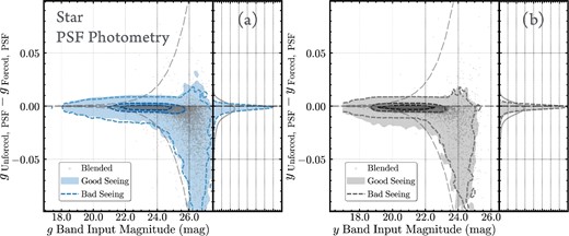
Magnitude differences between the unforced and forced PSF photometry for synthetic stars in the g (left) and y band (right). The lines and contour legends are identical to the plots in figure 5. (Color online)
The precisions and accuracies of forced PSF magnitudes shown here are summarized in table 1.
Summary of forced PSF magnitude.*
| Input | Filter | g | r | i | z | y | |||||
|---|---|---|---|---|---|---|---|---|---|---|---|
| magnitude | FWHM | 0|${^{\prime\prime}_{.}}$|45 | 0|${^{\prime\prime}_{.}}$|70 | 0|${^{\prime\prime}_{.}}$|45 | 0|${^{\prime\prime}_{.}}$|70 | 0|${^{\prime\prime}_{.}}$|45 | 0|${^{\prime\prime}_{.}}$|70 | 0|${^{\prime\prime}_{.}}$|45 | 0|${^{\prime\prime}_{.}}$|70 | 0|${^{\prime\prime}_{.}}$|45 | 0|${^{\prime\prime}_{.}}$|70 |
| (mag) | (mag) | (mag) | (mag) | (mag) | (mag) | (mag) | (mag) | (mag) | (mag) | (mag) | |
| 19.0 | σΔMag | 0.017 | 0.017 | 0.021 | 0.022 | 0.014 | 0.011 | 0.011 | 0.019 | 0.016 | 0.019 |
| 〈ΔMag〉 | 0.008 | 0.006 | 0.011 | 0.009 | 0.002 | 0.001 | 0.002 | 0.003 | 0.006 | 0.007 | |
| 20.0 | σΔMag | 0.018 | 0.018 | 0.023 | 0.025 | 0.015 | 0.012 | 0.012 | 0.020 | 0.017 | 0.019 |
| 〈ΔMag〉 | 0.009 | 0.005 | 0.011 | 0.009 | 0.002 | 0.002 | 0.003 | 0.003 | 0.006 | 0.008 | |
| 21.0 | σΔMag | 0.019 | 0.018 | 0.024 | 0.026 | 0.017 | 0.014 | 0.014 | 0.021 | 0.021 | 0.022 |
| 〈ΔMag〉 | 0.009 | 0.005 | 0.012 | 0.009 | 0.002 | 0.002 | 0.002 | 0.003 | 0.004 | 0.008 | |
| 22.0 | σΔMag | 0.023 | 0.020 | 0.025 | 0.029 | 0.018 | 0.015 | 0.017 | 0.024 | 0.035 | 0.037 |
| 〈ΔMag〉 | 0.009 | 0.005 | 0.011 | 0.009 | 0.002 | 0.002 | 0.003 | 0.004 | 0.006 | 0.006 | |
| 23.0 | σΔMag | 0.031 | 0.026 | 0.029 | 0.031 | 0.021 | 0.022 | 0.025 | 0.039 | 0.076 | 0.079 |
| 〈ΔMag〉 | 0.008 | 0.004 | 0.011 | 0.009 | 0.002 | 0.002 | 0.003 | 0.005 | −0.001 | 0.003 | |
| 24.0 | σΔMag | 0.049 | 0.038 | 0.036 | 0.046 | 0.030 | 0.046 | 0.056 | 0.082 | 0.147 | 0.146 |
| 〈ΔMag〉 | 0.007 | 0.003 | 0.010 | 0.007 | 0.002 | 0.001 | 0.005 | 0.003 | −0.003 | −0.033 | |
| 25.0 | σΔMag | 0.119 | 0.108 | 0.087 | 0.107 | 0.062 | 0.103 | 0.124 | 0.152 | – | – |
| 〈ΔMag〉 | −0.010 | −0.008 | 0.004 | 0.006 | 0.003 | −0.009 | −0.001 | −0.010 | – | – | |
*Summary of precisions and accuracies of forced PSF magnitudes in all five bands and in both goodSeeing (FWHM = 0|${^{\prime\prime}_{.}}$|45) and badSeeing (FWHM = 0|${^{\prime\prime}_{.}}$|70) tracts based on the statistics (standard deviation and mean value) of the difference between output forced PSF magnitude and input value (Δmag) shown in figure 5. Here, the precision is described using the standard deviation of Δmag within a series of input magnitude bins (σΔMag). The accuracy of PSF photometry in the same magnitude bin is described by the mean value of Δmag.
5.1.3 Precision and accuracy of PSF colors
PSF photometry is the most appropriate way to measure colors for point sources; therefore, the accuracy of the PSF color estimates is important to many scientific goals of the HSC survey (e.g., study of the Milky Way structure, selection of unique stellar objects or high-redshift quasars, and accurate star–galaxy separation).
In figure 7, we evaluate the precision and accuracy of the forced (g − i) and (i − y) PSF colors by comparing the differences between input and output colors (ΔColor) with both the input magnitudes and colors. Figure 7 shows that hscPipe provides precise and accurate PSF colors for synthetic stars with realistic color distributions down to very faint magnitudes. The average precision for (g − i) is ∼0.023 mag at iInput ∼ 19.0. The statistical scatter increases to ∼0.16 mag at iInput ∼ 25.0 mag. The (i − y) color displays similar precision. The forced PSF color measurements are not biased through the entire ranges of input magnitudes and colors.
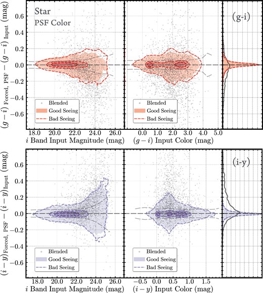
Accuracy of the color measurements for synthetic stars via the differences between input and forced PSF colors. The upper panels and lower panels are for g − i and i − y colors separately. The left-hand column shows the relation between input magnitude and the color difference, and the right-hand column uses the input colors as the x-axis instead. The lines and contour legends are identical to the plot in figure 5. (Color online)
Figure 7 shows that the precision of PSF colors does not depend on the seeing conditions. For instance, the precision of (g − i) for the badSeeing tract is only slightly worse at the very faint end (∼0.18 mag at iInput ∼ 25.0 mag) compared to the goodSeeing tract.
Figure 8 displays the precision of PSF colors by comparing the color distributions of the input sample to the recovered color distributions. Using four different colors and two color–color planes, we show that the forced PSF colors accurately recover the distributions of all four colors and the color–color distributions. On the (i − z)–(z − y) color plane, stars with extreme colors are not well recovered. The fraction of these stars is very low, and their poor recovery could relate to the scattered light in the y band that is still unaccounted for (see sub-subsection 5.8.14 of Aihara et al. 2018b).
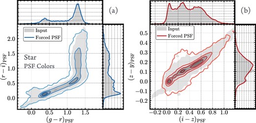
Evaluations of color measurement accuracy for synthetic stars using the color–color distributions. The plot on the left (a) uses (g − r) v.s. (r − i) colors, and the plot on the right (b) uses (i − z) and (z − y) colors. The filled contours and shaded histograms reflect the distributions for input colors. The empty contours and solid-line histograms show the distributions recovered by hscPipe. (Color online)
As for highly blended stars, figure 7 also shows that they have worse precision and accuracy in their colors compared to isolated stars. At fixed input magnitude, the precision in (g − i) is ∼0.1 mag worse for highly blended stars. Unlike PSF magnitudes, where the distributions of magnitude differences for highly–blended stars are clearly biased, the distributions of PSF color differences do peak around zero. However, the long asymmetric tails still indicate severe biases of PSF colors for blended stars: the (g − i) color is clearly biased towards bluer colors, while the (i − y) color shows a bias towards redder values. The performance of PSF magnitudes and colors are still poor for highly-blended stars in the current version of hscPipe. Object deblending becomes much more challenging at the depth of the HSC-SSP, and the current deblending algorithm is known to have limitations (see subsection 4.8 of Bosch et al. 2018) that could cause the problem shown here. The deblending algorithm is also being constantly updated now, and we will keep using SynPipe to evaluate its performance.
The statistical uncertainties of forced PSF colors are summarized in table 2. In figure 7, we also compare the SynPipe results with the uncertainties of the PSF color obtained by hscPipe (pair of grey long-dashed lines). Here, we simply add the magnitude errors from both bands in quadrature. We find that the average uncertainties of PSF color from hscPipe are consistent with the results of the SynPipe test. Again, we emphasize that the uncertainties of the PSF models are not taken into account.
Summary of forced PSF colors.*
| i Input | Color | (g − i) | (i − y) | ||
|---|---|---|---|---|---|
| FWHM | 0|${^{\prime\prime}_{.}}$|45 | 0|${^{\prime\prime}_{.}}$|70 | 0|${^{\prime\prime}_{.}}$|45 | 0|${^{\prime\prime}_{.}}$|70 | |
| (mag) | (mag) | (mag) | (mag) | (mag) | |
| 19.0 | σΔColor | 0.023 | 0.022 | 0.018 | 0.019 |
| 〈ΔColor〉 | 0.007 | 0.003 | −0.004 | −0.006 | |
| 20.0 | σΔColor | 0.028 | 0.024 | 0.019 | 0.019 |
| 〈ΔColor〉 | 0.007 | 0.003 | −0.004 | −0.006 | |
| 21.0 | σΔColor | 0.034 | 0.031 | 0.022 | 0.022 |
| 〈ΔColor〉 | 0.006 | 0.002 | −0.004 | −0.006 | |
| 22.0 | σΔColor | 0.053 | 0.051 | 0.031 | 0.030 |
| 〈ΔColor〉 | 0.004 | 0.001 | −0.004 | −0.005 | |
| 23.0 | σΔColor | 0.079 | 0.086 | 0.057 | 0.058 |
| 〈ΔColor〉 | −0.004 | −0.015 | −0.001 | −0.004 | |
| 24.0 | σΔColor | 0.116 | 0.122 | 0.111 | 0.112 |
| 〈ΔColor〉 | −0.015 | −0.001 | 0.009 | 0.004 | |
| 25.0 | σΔColor | 0.162 | 0.185 | 0.192 | 0.216 |
| 〈ΔColor〉 | 0.044 | −0.018 | 0.097 | 0.097 | |
*Summary of precisions and accuracies of forced PSF colors using (g − i) and (i − y) colors and in both goodSeeing (FWHM = 0|${^{\prime\prime}_{.}}$|45) and badSeeing (FWHM = 0|${^{\prime\prime}_{.}}$|70) tracts based on the standard deviation and mean value of the difference between output forced PSF color and input value (ΔColor) shown in figure 7. Here, we describe the precision and accuracy of PSF color measurements using the standard deviation and mean values of ΔColor in bins of input i-band magnitudes.
5.2 cModel photometry of galaxies
For galaxies, hscPipe uses a CModel photometry algorithm that is an improved version of the SDSS CModel photometry. For details about the CModel algorithm, please see description in subsection 2.2 and Bosch et al. (2018). Despite the limitations of the CModel method (e.g., sensitivity to the background subtraction and to deblending failures), it can deliver robust PSF-corrected fluxes and colors for galaxies.
A typical tract in the Wide layer contains ∼400000 extended objects with iCModel < 25.5 mag. We randomly inject ∼40000 synthetic galaxies (additional ∼10%) into each tract, and will not create an over-crowded situation. Using a similar approach for synthetic stars, we select galaxy samples for photometric comparisons. Synthetic galaxies that are located within 2 pixels of the centroids of real objects are removed from the sample (they represent ∼3%–7% of the input sample). After imposing quality cuts on the recovered synthetic galaxy sample (see appendix 1 for details), we have ∼30000 galaxies in each tract.
We find that hscPipe mis-classifies fewer than 1% of these objects as point sources in the goodSeeing tract. However, the fraction of misclassified galaxies increases to 4% in the goodSeeing tract. We will discuss star/galaxy separation further in subsection 6.2.
We define a sample of highly-blended galaxies by imposing the cut b > 0.05.18 Due to the extended nature of galaxies, the b distribution of synthetic galaxies is more skewed toward high values (especially for the badSeeingtract) compared to the b distribution of stars. About 7%–9% of synthetic galaxies are highly blended, with b > 0.05. The fraction is slightly higher in the badSeeing tract, and therefore the g band also has higher fraction of highly-blended galaxies. In our plots, we will highlight highly-blended galaxies and will discuss blending effects further in subsection 6.3.
5.2.1 Input magnitude and the S/N of CModel photometry
Figure 9 shows the relation between the input magnitudes and the S/N of synthetic galaxies. The S/N is the ratio of the CModel flux and the flux error measured by hscPipe. For an extended object with a wide variety of light profiles, the definition of S/N is not as straightforward as for point sources. Here the adopted S/N corresponds to the average S/N over the entire footprint. The center of the galaxy typically has higher S/N than this value. We adopt this definition, as the main purpose here is to demonstrate the overall “significance” of the galaxy detections down to a certain magnitude.
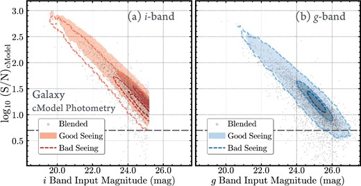
Relation between input magnitudes (left: i band; right: g band) of synthetic galaxies log (S/N) as measured by hscPipe CModel photometry. Lines and contours are similar to figure 4. The truncation in the i-band input magnitude is caused by the magnitude limit of COSMOS galaxies used in this test. (Color online)
Figure 9 shows that the CModel photometry displays a well-behaved relation between input magnitude and output S/N. Compared to stars, the S/N from CModel for synthetic galaxies shows a larger scatter at fixed input magnitude. This is likely due to the fact that galaxies have a wider range in sizes and shapes than point sources. In the i band, a typical 25.2 mag galaxy has S/N ∼ 20 from CModel, but there are also galaxies at the same magnitude which have S/N below 5. The HSC Wide layer can detect galaxies as faint as i ∼ 26.0 mag but the sample becomes incomplete at these faint magnitudes. This also introduces a selection bias if galaxies with certain structural properties (e.g., more extended and lower surface brightness) are harder to detect than others. HSC survey data users who want to select flux-limited galaxy samples, or who intend to study the population of faint (e.g., high-z) galaxies should keep this in mind. Finally, we also find that a worse seeing leads to a lower S/N at fixed magnitude (see figure 4 for the i band).
The CModel flux error also only considers statistical uncertainties provided by the variance information. For galaxy photometry based on a 2D model, its quite often that the true error budget is dominated by systematic effects during the fitting process (e.g., choice of model assumption, priors for parameters, uncertainty of PSF model, and uncertainty in background subtraction). Therefore, statistical tests like the one presented here can provide more insights about the accuracy of CModel photometry.
5.2.2 Precision and accuracy of the CModel magnitude
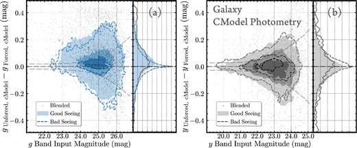
Figure 10 shows the precision (σΔMag) and accuracy (〈ΔMag〉) of CModel magnitude in each band using the same format as figure 5.

Accuracies of the hscPipe CModel photometry for synthetic galaxies measured by the difference between input and output forced CModel magnitudes. Plots (a), (b), (c), (d), and (e) show the results for the g, r, i, z, and y bands, respectively. The lines and contour legends are identical to figure 5. (Color online)
The overall performance of CModel photometry is reasonable down to iInput = 25.2 mag. Compared to the PSF photometry for stars, the statistical uncertainties of CModel magnitudes are larger for galaxies, which is expected given the diversity of galaxy shapes and sizes that adds complexity to the model-fitting process. At the same time, figure 10 shows that the CModel algorithm in hscPipe provides unbiased and consistent photometry for galaxies across different bands and seeing conditions.
The typical precision of the i-band flux using forced CModel is at the ∼10%–14% level in the goodSeeing tract at iInput < 24.0 mag. It moderately degrades to ∼18% at 25.0 mag. The performance is similar in the i band for the badSeeing tract. At 20.0 < iInput < 24.0 mag, the accuracies of forced CModel magnitudes change between + 0.017 mag to −0.023 mag. At 24.0 < iInput < 25.5 mag, 〈ΔMag〉 is around −0.006 mag, which suggest that forced CModel photometry is unbiased down to the very faint end.
It is worth noting that the flux uncertainty from SynPipe are significantly larger than the flux errors from hscPipe, which does not take into account the systematic uncertainties involved in the modeling fitting process. Even though our synthetic galaxy sample is composed of objects with simple single-Sérsic models, the CModel algorithm can only approximate them to a certain accuracy because of the background noise, deblending uncertainties, and priors imposed on model parameters. Given that real galaxies are more complex in structure, our quoted uncertainties should be treated as lower limits.
The precision of forced CModel photometry is consistent across all filters. For the g, r, and z bands, the statistical uncertainties are very similar to i-band results between 20.0 and 25.0 mag. The forced CModel magnitudes are also unbiased for these three filters across the entire input magnitude range. The precision for the y band is slightly worse, ranging from 10% to 17% in the same magnitude bins. In addition, the forced CModel tends to overestimate the total flux in the y band at >24.0 mag. This bias in the y-band flux is equal to −0.07 mag at 24.0 mag to −0.22 mag at 25.0 mag. Worse seeing conditions and a higher background noise level mean that it is more difficult to detect faint objects in the y band. At yInput ∼ 24.0, the average S/N for CModel is already around the detection threshold.
Our synthetic galaxy sample is dominated by faint galaxies (iInput > 24.0 mag) that are crucial to key scientific goals of the HSC survey. However, it also means poor statistics for bright galaxies. We do find that at iInput < 20.0 the forced CModel photometry starts to systematically underestimate total fluxes. Based on external comparisons, the behavior of CModel for bright galaxies may depend on galaxy types (e.g., Aihara et al. 2018b). Also, at the bright end, another known issue is that the current hscPipe over-deblends around bright objects. Inappropriately weighted priors in CModel also lead to poorer photometric quality for bright galaxies. Finally, at the imaging depth of HSC (>29.0 mag arcsec−2 in the Wide layer i band), CModel may simply not be a good choice for modeling bright galaxies (e.g., massive elliptical galaxies; see Huang et al. 2017 for more details).
We also find that highly-blended galaxies tend to have systematically underestimated total fluxes (with an average offset ∼0.1 mag) and higher statistical uncertainties in all five bands. However, the contrast between relatively isolated and highly-blended galaxies in photometric performance is not as stark as for synthetic stars (figure 5).
We also test the unforced CModel photometry in all five bands, and the results suggest similar precision. Figure 11 compares the difference between forced and unforcedCModel in the g and y bands. The main noticeable trend is that galaxies brighter than 24.0 mag in the g band have systematically brighter forced CModel magnitudes, which suggests that the forced CModel is more accurate in the g band as the model parameters are determined using bands with higher S/N.
Magnitude differences between the unforced and forced CModel photometry for synthetic galaxies in the g (left) and y band (right). The lines and contour legends are identical to the plots in figure 6. (Color online)
The precisions and accuracies of forced CModel magnitudes shown here are summarized in table 3. Similar to PSF photometry, here we also compare the average CModel magnitude error provided by hscPipe in each magnitude bin with our SynPipe test results (pairs of grey long-dashed lines on each plot). The CModel magnitude error in hscPipe only considers the statistical uncertainties based on the variance information. Apparently, the CModel flux uncertainties from hscPipe underestimate the true uncertainty of the photometry. Although it is possible that hscPipe is too optimistic about the statistical uncertainties (e.g., correlated noise across pixels), the more likely situation is still that the real error budget of the CModel magnitude is dominated by systematics in the model fitting process. We stress that users of CModel photometry should take this into consideration.
Summary of forced CModel magnitude.*
| Input | Filter | g | r | i | z | y | |||||
|---|---|---|---|---|---|---|---|---|---|---|---|
| magnitude | FWHM | 0|${^{\prime\prime}_{.}}$|45 | 0|${^{\prime\prime}_{.}}$|70 | 0|${^{\prime\prime}_{.}}$|45 | 0|${^{\prime\prime}_{.}}$|70 | 0|${^{\prime\prime}_{.}}$|45 | 0|${^{\prime\prime}_{.}}$|70 | 0|${^{\prime\prime}_{.}}$|45 | 0|${^{\prime\prime}_{.}}$|70 | 0|${^{\prime\prime}_{.}}$|45 | 0|${^{\prime\prime}_{.}}$|70 |
| (mag) | (mag) | (mag) | (mag) | (mag) | (mag) | (mag) | (mag) | (mag) | (mag) | (mag) | |
| 20.0 | σΔMag | 0.111 | 0.137 | 0.197 | 0.167 | 0.173 | 0.154 | 0.171 | 0.168 | 0.179 | 0.169 |
| 〈ΔMag〉 | −0.006 | 0.018 | −0.036 | −0.024 | −0.023 | 0.017 | −0.006 | 0.027 | 0.011 | 0.041 | |
| 21.0 | σΔMag | 0.156 | 0.161 | 0.151 | 0.119 | 0.157 | 0.157 | 0.176 | 0.155 | 0.169 | 0.164 |
| 〈ΔMag〉 | −0.036 | −0.008 | −0.015 | 0.023 | 0.008 | 0.043 | 0.043 | 0.046 | 0.056 | 0.052 | |
| 22.0 | σΔMag | 0.161 | 0.138 | 0.147 | 0.142 | 0.154 | 0.153 | 0.165 | 0.167 | 0.178 | 0.169 |
| 〈ΔMag〉 | −0.004 | 0.029 | 0.033 | 0.050 | 0.004 | 0.040 | 0.038 | 0.045 | 0.044 | 0.048 | |
| 23.0 | σΔMag | 0.152 | 0.147 | 0.167 | 0.168 | 0.168 | 0.174 | 0.182 | 0.185 | 0.197 | 0.194 |
| 〈ΔMag〉 | 0.021 | 0.040 | 0.033 | 0.036 | 0.017 | 0.021 | 0.018 | 0.028 | 0.014 | 0.020 | |
| 24.0 | σΔMag | 0.176 | 0.181 | 0.179 | 0.189 | 0.183 | 0.193 | 0.201 | 0.222 | 0.241 | 0.253 |
| 〈ΔMag〉 | 0.009 | 0.028 | 0.028 | 0.025 | −0.001 | 0.003 | −0.002 | 0.009 | −0.067 | −0.057 | |
| 25.0 | σΔMag | 0.196 | 0.202 | 0.211 | 0.232 | 0.218 | 0.246 | 0.241 | 0.278 | 0.308 | 0.315 |
| 〈ΔMag〉 | −0.005 | 0.012 | 0.012 | 0.022 | −0.006 | −0.013 | −0.012 | −0.034 | −0.224 | −0.299 | |
*Summary of precisions and accuracies of forced CModel magnitudes in all five bands and in both goodSeeing (FWHM = 0|${^{\prime\prime}_{.}}$|45) and badSeeing (FWHM = 0|${^{\prime\prime}_{.}}$|70) tracts based on the standard deviation and mean value of the difference between output forced CModel magnitude and input value (Δmag) shown in figure 10. Other details are the same as in table 1.
5.2.3 Precision and accuracy of the CModel color
Precise and unbiased five-band CModel colors from hscPipe are crucial for photometric redshift estimates and spectral energy distribution (SED) fitting results. They are also key, for example, to the selection of high-z Lyman-break galaxies (LBG).
Figure 12 evaluates the precision and accuracy of forced (g − i) and (i − y) CModel colors using the same format as figure 7. We find that hscPipe provides reliable CModel colors for synthetic galaxies down to iInput ∼ 25.0 mag. For (g − i) colors, the statistical uncertainty at iInput ∼ 20.0 mag is ∼0.07 mag. The statistical uncertainty increases to ∼0.18 mag at iInput ∼ 25.0 mag. The (i − y) colors show similar results, except the precision at iInput > 24.0 mag becomes slightly worse.
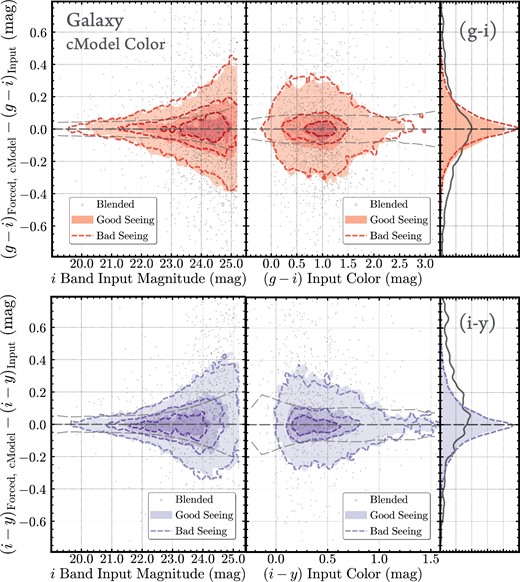
Accuracies of the color measurements for synthetic galaxies via the differences between input and forced CModel colors. The upper panels and lower panels are for g − i and i − y colors separately. The left-hand column shows the relation between input magnitude (x-axis) and the color difference, and the right-hand column uses the input colors as the x-axis. The lines and contour legends are identical to the plot in figure 7. (Color online)
The performance of forced CModel color does not strongly depend on seeing and is unbiased for the entire range of magnitudes and colors that we have tested. The only noticeable feature is that the (i − y) color at iInput > 24.0 is systematically redder than the real values by + 0.05 mag. As mentioned above, this is not surprising given the shallower y-band imaging depth. Highly-blended galaxies are less precise in their forced CModel colors compared to isolated galaxies and on average show slightly bluer (g − i) colors and redder (i − y) colors compared to their input colors.
Figure 13 compares the input color–color distributions with the recovered ones. The general 2D distributions are well-recovered but the precision is not as good as for stars, especially in the (i − z) vs. (z − y) plane. This is expected given the narrow dynamical ranges of these colors in the redder filters. The forced CModel tends to slightly underestimate the (g − r) and (i − z) colors at the very “blue” end, while overestimating the (z − y) color at the very red end. The same y-band scattered light issue also affects the CModel photometry. The background levels are also higher in the z and y bands, which could lead to higher uncertainties from background subtraction. Unfortunately, SynPipe is not yet equipped to test the impact of background subtraction on photometry, and the issues with the (z − y) colors will be investigated later.
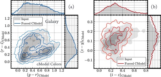
Color–color distributions of synthetic galaxies. The panel (a) uses (g − r) vs. (r − i) colors, and the panel (b) uses (i − z) and (z − y) colors. Filled contours and shaded histograms correspond to the input colors. Empty contours and solid-line histograms show the distributions recovered by hscPipe CModel photometry. (Color online)
We note that our synthetic galaxies do not have color gradients. In reality, color gradients will complicate the situation and hence the statistical uncertainties shown here should be considered as lower limits.
The statistical uncertainties of forced CModel colors are summarized in table 4. We also compare the CModel color uncertainties estimated by hscPipe with our SynPipe results. We still simply add the magnitude error from each band in quadrature. For the (g − i) color, we see that the statistical uncertainties of CModel colors are very similar to the SynPipe results. This is consistent with the design of the forced CModel algorithm, where precisions are expected to be much better for colors than for fluxes themselves (see sub-subsection 4.9.9 of Bosch et al. 2018). For the (i − y) color, we can draw a similar conclusion except for at the faint end (i > 24.0 mag), where the uncertainties from SynPipe test become higher than the statistical uncertainties from hscPipe. This is likely due to the scattered light in the y band that has not been accounted for (see sub-subsection 5.8.14 in Aihara et al. 2018b).
Summary of forced CModel colors.*
| i Input | Color | (g − i) | (i − y) | ||
|---|---|---|---|---|---|
| FWHM | 0|${^{\prime\prime}_{.}}$|45 | 0|${^{\prime\prime}_{.}}$|70 | 0|${^{\prime\prime}_{.}}$|45 | 0|${^{\prime\prime}_{.}}$|70 | |
| (mag) | (mag) | (mag) | (mag) | (mag) | |
| 20.0 | σΔColor | 0.068 | 0.051 | 0.072 | 0.046 |
| 〈ΔColor〉 | 0.013 | 0.002 | −0.006 | −0.001 | |
| 21.0 | σΔColor | 0.080 | 0.059 | 0.062 | 0.040 |
| 〈ΔColor〉 | 0.010 | 0.003 | −0.003 | −0.004 | |
| 22.0 | σΔColor | 0.089 | 0.072 | 0.071 | 0.059 |
| 〈ΔColor〉 | 0.002 | 0.002 | −0.005 | −0.007 | |
| 23.0 | σΔColor | 0.105 | 0.090 | 0.109 | 0.103 |
| 〈ΔColor〉 | −0.018 | 0.001 | −0.002 | −0.005 | |
| 24.0 | σΔColor | 0.136 | 0.127 | 0.175 | 0.170 |
| 〈ΔColor〉 | −0.008 | 0.006 | 0.012 | −0.007 | |
| 25.0 | σΔColor | 0.179 | 0.185 | 0.227 | 0.241 |
| 〈ΔColor〉 | −0.003 | 0.019 | 0.053 | 0.006 | |
*Summary of precisions and accuracies of forced CModel colors using (g − i) and (i − y) colors and in both goodSeeing (FWHM = 0|${^{\prime\prime}_{.}}$|45) and badSeeing (FWHM = 0|${^{\prime\prime}_{.}}$|70) tracts based on the standard deviation and mean value of the difference between output forced CModel color and input value (ΔColor) shown in figure 12. Other details are the same as in table 2.
6 Other performance tests
In this section, we turn our attention to astrometric calibration, star–galaxy separation, blending effects, and galaxy shape measurements.
6.1 Astrometric calibration
We inject synthetic objects into single-visit images using the initial (and less accurate) astrometric calibration. During the image-stacking step, the joint calibration process improves the astrometric solutions. Therefore, differences between the input and output coordinates from SynPipe can help us understand how much the joint calibration step changes the astrometric calibration, and how well hscPipe can measure the central coordinates of stars and galaxies.
Figure 14 shows the distribution of astrometric offsets for synthetic stars and galaxies in goodSeeing and badSeeingtracts. Note that HSC coadd image has pixel size of 0|${^{\prime\prime}_{.}}$|168 per pixel. We find small systematic offsets at the ∼10–20 mas level, which is similar to the uncertainties of astrometric calibration quoted in Aihara et al. (2018b). The two tracts show different systematic offsets, while the synthetic stars and galaxies show coherent offsets in the same tract. This shows that the initial astrometric calibration of HSC has very reasonable accuracy. It also suggests that hscPipe can find the centroids of stars and galaxies with precisions that are consistent with the astrometric calibration uncertainty under moderately different seeing conditions.
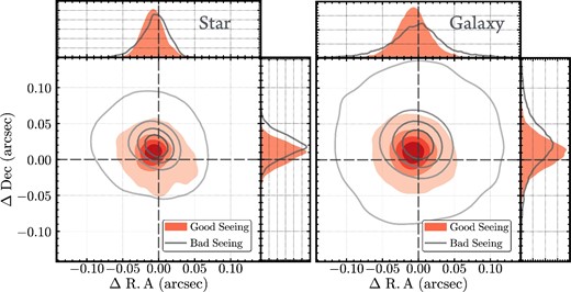
Astrometric accuracy for synthetic stars (left) and galaxies (right). We show the differences between the input RA and Dec and the coordinates measured on the coadd images. HSC coadd image has pixel scale of 0|${^{\prime\prime}_{.}}$|168 per pixel. Filled contours (filled histogram) and open contours (solid-line histogram) are for synthetic objects from tracts with good and bad seeing conditions, respectively. ΔRA = 0 and ΔDec = 0 are marked by dashed lines. This shows that the initial astrometric calibration is already very accurate, and it also suggests that hscPipe can find the centroids of stars and galaxies with precisions that are consistent with the astrometric calibration uncertainty under moderately different seeing conditions. (Color online)
6.2 Star–galaxy separation
Star–galaxy separation becomes increasingly difficult at faint magnitudes (i < 24.0 mag). In hscPipe, the star–galaxy classification primarily depends on the extendedness value, which is measured by the magnitude difference between PSF and CModel photometry in the i band. This method has limitations and only works well down to i ∼ 24 mag (see sub-subsection 4.9.10 of Bosch et al. 2018). For fainter extended objects, the difference between these two magnitudes become seeing- and model-dependent. Moreover, right now, hscPipe simply uses (mPSF − mCModel) > 0.0164 mag to separate star and galaxies.
Figure 15 shows the current status of our star–galaxy classification scheme. Figure 15 shows the difference between PSF and CModel magnitudes as a function of input magnitude. We find that 20% of synthetic stars at iInput > 23.0 mag are misclassified as extended objects, while only a tiny fraction of faint synthetic galaxies (iInput > 24.0) are misclassified as stars. This confirms that the current star–galaxy classification strategy in hscPipe results in a galaxy sample with high completeness and a star sample with high purity. It is also clear that the seeing condition strongly modifies the distributions of iPSF − icModel. Worse seeing conditions make star–galaxy separation more challenging. The completeness and purity of galaxy and star samples at the faint end will depend on seeing conditions. In Aihara et al. (2018b), the star–galaxy separation issue is tested in a small field but under different seeing conditions and imaging depths (see their subsection 5.7). The overall conclusions are the same as ours: the efficiency and accuracy of the current star–galaxy separation algorithm are reasonable at i < 23.0 mag, but depend on both seeing and depth. We should point out that careful evaluation of star–galaxy separation algorithm and the completeness of both types of objects are important to several scientific topics of HSC-SSP. The accuracy of star-galaxy separation should be tested on a larger scale, in a way that covers different observational conditions and with a higher number density of objects. This will be a major effort and is beyond the scope of this work. At the same time, hscPipe will replace the current star–galaxy separation algorithm with a much improved version that provides an actual probability of being star or galaxy (also see sub-subsection 4.9.10 in Bosch et al. 2018). It will be available for the future data release, and will be tested using SynPipe.
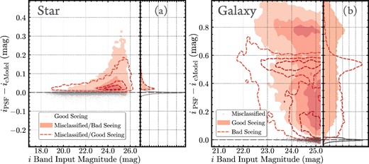
Evaluation of the hscPipe star–galaxy separation scheme. Star–galaxy separation is based on the the magnitude difference between the PSF and CModel photometry. The plot on the panel (a) corresponds to synthetic stars. Filled contours and the filled histogram show distributions of correctly classified synthetic stars in the goodSeeing tract. The scatter plot (dashed-line histogram) and open contours (solid-line histogram) show distributions of synthetic stars that are misclassified as extended objects in tracts with bad and good seeing conditions, respectively. The plot on the panel (b) corresponds to synthetic galaxies. Filled contours (filled histogram) and open contours (solid-line histogram) are for galaxies from goodSeeing and badSeeing tracts, respectively. The scatter plot and dashed-line histogram highlight synthetic galaxies that are misclassified as point sources. (Color online)
6.3 Blending effects
Figure 16 shows the b parameter versus the difference between input and output values for both magnitudes and colors. For both PSF and CModel magnitude distributions, we can see clear trends that total fluxes are systematically underestimated for highly blended (b > 0.05) objects. This effect is particularly strong for stars.
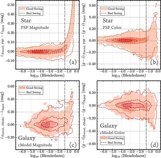
Relation between the log10(Blendedness) parameter and the photometric accuracy of synthetic stars (upper row, a and b) and galaxies (lower row, c and d). Left-hand columns (a and c) show the uncertainties in PSF and/or CModel magnitudes. Right-hand columns (b and d) show the uncertainties in (g − i) colors. Filled contours and open contours show results for goodSeeing and badSeeing tracts, respectively. log10(Blendedness) = −1.0 is marked using a vertical dashed line. (Color online)
As for colors, higher values of b result in higher statistical uncertainties for both stars and galaxies, but the trends are different for each. Highly-blended stars have clearly redder (g − i) colors than the input values. Highly-blended galaxies seem to have (g − i) colors that are bluer than the true values.
Blendedness-related uncertainties are not included in the photometric errors released by hscPipe. We therefore remind HSC users to treat any highly-blended object with greater caution.
6.4 Shape and structural parameters of galaxies
In SDSS, structural parameters like size and shape from CModel are often used to study the evolution galaxies. Although the CModel in hscPipe follows a similar algorithm, its primary goal now is to provide accurate and consistent magnitude and color in all five bands for a vast majority of faint, small galaxies. To improve the stability of CModel for these low-S/N and barely resolved galaxies, hscPipe uses Bayesian priors on galaxy sizes and axis ratios. However, the current implementation of these priors has a serious bug and leads to severely underestimated sizes and ellipticities of galaxies.
Figure 17 demonstrates this issue and compares the input and measured values of the CModel axis ratio. Here, (b/a)CModel is the flux-weighted sum of the axis ratios estimated by exponential and de Vaucouleurs models.
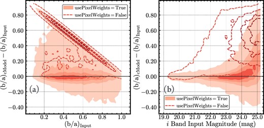
Accuracy of weighted axis ratio estimates for synthetic galaxies using CModel photometry. The left-hand plot (a) shows the relation between the input (b/a) and the uncertainty in (b/a). The right-hand plot (b) shows the relation between input magnitude and the uncertainty in (b/a). Open contours are for the default test with usePixelWeights=False, and filled contours correspond to usePixelWeights=True. (Color online)
Using our SynPipe tests, we discovered that the bug related to the priors only presents when usePixelWeight configuration is set to False during the data reduction. Please see Bosch et al. (2018; sub-subsection 4.4.9 and appendix 2) for more details about the fitting algorithm of CModel. In short, when usePixelWeight is set to True, the CModel algorithm will use the per pixel square root of the variance map for coadd image as weights during the fitting. When usePixelWeight is False, a constant weight will be used instead. As one can see, this leads to significantly overestimated axis ratios for almost all galaxies.19 We repeat the SynPipe run for galaxies with usePixelWeight =True, and this change clearly mitigates the problem. When we use usePixelWeight =True, (b/a)CModel provides an unbiased axis ratio estimation for galaxies with iInput < 24.0 mag. This change is still related to the bug in priors. The actual effect of using per-pixel variance should be very small. The next version of hscPipe will fix this bug, and SynPipe will help evaluate the precisions of shape and size measurements. This is a good example that demonstrates how the SynPipe framework is valuable for quality control and that it can be used to improve hscPipe.
For the current HSC data release, we warn users against using the sizes and shapes from CModel to study the structural properties of galaxies.
7 Discussion
Motivated mainly by observational cosmology and time-domain astrophysics, we are witnessing an exciting time for modern imaging surveys. Increasingly sophisticated observational strategies and complex data reduction processes adopted by these surveys require careful tests to understand the dominant systematic issues and thoroughly evaluate the quality of scientific catalogs. In this work, we present SynPipe, a Python-based framework to test the performance of hscPipe for the HSC-SSP.
Similar tools have been developed for DES (The Dark Energy Survey Collaboration 2005). For instance, Chang et al. (2015) designed a forward-modeling simulation framework to test the “transfer function” (from photons to tabulated photometric measurements) of DES data reduction pipeline using simulated images. In a different effort, Suchyta et al. (2016) developed BALROG, a software that characterizes measurement biases in DES data reduction by injecting fake objects on the coadded DES images. Compared to these studies, the main advantage of SynPipe is that it enables us to conduct tests in real galaxy images using the same pipeline as used for science purposes. It injects synthetic objects to real single-exposure images, and follows the entire data reduction process (including image warping and stacking process) make sure that all realistic features on the image and systematics in each step of data reduction can be taken into account.
Here we focused on characterizing the photometric performance of hscPipe. However, SynPipe is a flexible tool and is being used for a range of other applications. For instance, R. Murata et al. (in preparation) use SynPipe to characterize the level of blending in the HSC Wide layer. Niikura et al. (2017) apply SynPipe to high-cadence HSC observations of M31 HSC images to search for microlensing events. SynPipe is also currently being used to estimate the completeness of high-z LBG and Lyman-α emitters (Ono et al. in preparation; Konno et al. in preparation), to check the completeness of high-z LBG pairs as a function of pair separation (Harikane et al. in preparation), to test the completeness of low surface–brightness dwarf galaxies selections (Greco et al. 2017), and to test magnification effects around nearby clusters (I.-N. Chiu et al. in preparation). Moreover, SynPipe is now being incorporated into the data reduction pipeline for LSST, and will also be used to test its performance in the future.
Both hscPipe and SynPipe are undergoing active development and still face certain limitations. Currently, SynPipe cannot test the impact of background subtraction and PSF modelling on the performance of photometry. For a more comprehensive summary of the current caveats of HSC data, please see subsection 5.8 of Aihara et al. (2018b). In the following section, we summarize the issues with hscPipe that have been identified by our SynPipe tests.
In the near future, we plan to update SynPipe to provide a photometric benchmark for each HSC-SSP data release to help improve hscPipe. At the same time, we are also working on improving the efficiency of SynPipe. Many users are not necessarily concerned with the subtle effects involved in the image stacking process. Hence, a future implementation of SynPipe will include the option of injecting objects directly on to coadd images, which will speed up the generation of synthetic data sets.
8 Summary and conclusion
In February 2017, the HSC survey made its first public data release, and the survey continues to produce increasingly larger amounts of high-quality imaging data. To help achieve the designed goals of the survey and to facilitate scientific investigations, we have developed SynPipe, a flexible framework based on hscPipe that can be used to perform quality control on the HSC pipeline outputs. SynPipe operates by injecting synthetic stars and galaxies into single-visit images. These data are then processed by hscPipe to generate coadd images and to perform photometric measurements. With this approach, SynPipe can be used as an end-to-end and realistic test of the full data reduction process. In this paper, we use two tracts in the HSC Wide layer with representative seeing conditions (goodSeeing with FWHM = 0|${^{\prime\prime}_{.}}$|45 seeing; badSeeing with FWHM = 0|${^{\prime\prime}_{.}}$|70 seeing) to test the general behaviors of HSC photometry for both stars and galaxies. The results shown in this paper demonstrate the utility of the SynPipe framework in order to perform end-to-end quality control on pipeline products to the level of accuracy needed by large panchromatic surveys.
Our main findings are the following:
The forced PSF photometry provides precise and accurate measurements of magnitude and color for isolated stars at 18.0 < i < 25.0. The typical statistical uncertainties of HSC forced PSF photometry for stars ranges from 0.01 mag at i ∼ 18.0 mag to 0.08 mag at i ∼ 25.0 mag (1%–7% precision in the i band). The forced PSF photometry can accurately recover the color–color sequences of stars.
The forced CModel photometry is reliable for synthetic galaxies with realistic distributions of structural parameters and colors at 20.0 < i < 25.0 mag. The statistical uncertainties of forced CModel magnitude ranges from ∼7% at i ∼ 20.0 mag to ∼10% at i ∼ 25.0 mag. The forced CModel colors for galaxies are precise and are consistent across in all five bands. They also do not show biases with input magnitudes and colors.
The forced PSF and CModel photometry are robust against moderate changes in the seeing conditions, despite the fact that worse seeing leads to a lower S/N at fixed input magnitude.
Blending (b > 0.05) has an impact on the accuracy of both PSF and CModel photometry, especially for stars. For highly blended stars, the forced PSF photometry overestimates the magnitudes of stars on average by 0.1–0.2 mag. For galaxies, blending effects typically add an additional 0.05-mag statistical uncertainty in both magnitude and color estimates.
We also highlight several known issues with the current version of hscPipe:
The performance of the current star–galaxy separation algorithm in hscPipe is not perfect, and degrades at fainter magnitudes and with poor seeing conditions. The fraction of stars that are misclassified as extended objects is still quite high. >20% of the synthetic stars at i > 22.5 mag are misclassified.20
The bug in priors on structural parameters and the usePixelWeights=False nominal setting in CModel result in very biased estimates of the shapes and sizes for galaxies. The axis ratio from CModel is highly overestimated and the effective radius is typically underestimated. This issue hence can also affect the accuracy of star–galaxy classification.
The HSC collaboration is working on improving these issues for future versions of hscPipe and for subsequent data releases.
Acknowledgements
The Hyper Suprime-Cam (HSC) collaboration includes the astronomical communities of Japan and Taiwan, and Princeton University. The HSC instrumentation and software were developed by the National Astronomical Observatory of Japan (NAOJ), Kavli Institute for the Physics and Mathematics of the Universe (Kavli IPMU), University of Tokyo, High Energy Accelerator Research Organization (KEK) in Japan, Academia Sinica Institute for Astronomy and Astrophysics (ASIAA) in Taiwan, and Princeton University in the United States. Funding was contributed by the FIRST program from Japanese Cabinet Office; Ministry of Education, Culture, Sports, Science and Technology (MEXT); Japan Society for the Promotion of Science (JSPS); Japan Science and Technology Agency (JST); Toray Science Foundation; NAOJ; Kavli IPMU; KEK; ASIAA; and Princeton University.
This paper makes use of software developed for the Large Synoptic Survey Telescope. We thank the LSST Project for making their code available as free software at 〈http://dm.lsstcorp.org〉.
This work is in part supported by JSPS KAKENHI (Grant Number 26800093, 15H03654, and JP17H01131) as well as a MEXT Grant-in-Aid for Scientific Research on Innovative Areas (Nos. 15H05887, 15H05892, 15H05893, 15K21733). RM is supported by the US Department of Energy Early Career Award Program. RyM is financially supported by the University of Tokyo-Princeton strategic partnership grant and Advanced Leading Graduate Course for Photon Science (ALPS).
Pan-STARRS1 Surveys (PS1) have been made possible through contributions of Institute for Astronomy, University of Hawaii, Pan-STARRS Project Office, Max-Planck Society and its participating institutes (Max Planck Institute for Astronomy, Heidelberg, and Max Planck Institute for Extraterrestrial Physics, Garching), Johns Hopkins University, Durham University, University of Edinburgh, Queen’s University Belfast, Harvard-Smithsonian Center for Astrophysics, Las Cumbres Observatory Global Telescope Network Incorporated, National Central University of Taiwan, Space Telescope Science Institute, National Aeronautics and Space Administration under Grant No. NNX08AR22G issued through Planetary Science Division of NASA Science Mission Directorate, National Science Foundation under Grant No. AST-1238877, University of Maryland, Eötvös Lorand University (ELTE), and Los Alamos National Laboratory.
This research made use of Astropy, a community-developed core Python package for Astronomy (Astropy Collaboration et al. 2013; 〈http://www.astropy.org/〉); astroML, a machine learning library for astrophysics (VanderPlas et al. 2014; 〈http://www.astroml.org/〉); SciPy, an open source scientific tool for Python (E. Jones et al. 2001, SciPy: Open source scientific tools for Python; 〈http://www.scipy.org/〉); NumPy, a fundamental package for scientific computing with Python (van der Walt et al. 2011; 〈http://www.numpy.org/〉); Matplotlib, a 2-D plotting library for Python (Hunter 2007; 〈http://matplotlib.org/〉); and scikit-learn, a machine learning library in Python (Pedregosa et al. 2011; 〈http://scikit-learn.org/〉).
Appendix 1. Quality control of synthetic objects
We apply quality control to the stars and galaxies selected from the HSC UltraDeep COSMOS fields before we match them with the stars and models for galaxies from the HST/ACS COSMOS data. The same quality control criteria are also used to select synthetic stars and galaxies from the SynPipe results before we perform photometric comparisons.
To select synthetic stars and galaxies from the HSC survey data in order to test the photometry, we apply some basic quality control cuts.
The HSC survey defines the full–depth and full–color regions (FDFC) to ensure the data used for science reach the expected number of exposures in each band [|$\mathtt {(\#gri\ \ge \ 4)\ and\ (\#yz\ \ge \ 6)\ and\ (Limiting\ imag> 25.6)}$|; see Aihara et al. (2018b) for details]. Since the two tracts we used in this work are almost entirely covered in the FDFC region, we did not apply this cut.
First, we make sure the object is a “primary” detection (in the inner part of tract and patch; not a parent in the deblending process), is successfully deblended, has reliable centroid, and is not bothered by various optical issues:
detect_is_primary==True
deblend_skipped==False
deblend_nchild=0
[grizy]flags_badcentroid==False
[grizy]centroid_sdss_flags==False
[grizy]flags_pixel_edge==False
[grizy]flags_pixel_interpolated_center==False
[grizy]flags_pixel_saturated_center==False
[grizy]flags_pixel_cr_center==False
[grizy]flags_pixel_bad==False
[grizy]flags_pixel_suspect_center==False
[grizy]flags_pixel_clipped_any==False
[grizy]flags_pixel_bright_object_center==False
For stars, we ensure the selected objects have useful PSF magnitudes:
[grizy]flux_psf_flags==False
For galaxies, we also make sure useful CModel photometry is available:
[grizy]cmodel_flux_flags==False
Appendix 2. b: The blendedness parameter
To evaluate the degree to which an object is blended with others, hscPipe introduces the blendedness parameter: b ([grizy]blendedness_abs_flux). We briefly define b below; please refer to Bosch et al. (2018) and R. Murata et al. (in preparation) for more details.
By definition, the parameter is bound from 0 to 1. When the deblending process is carried out correctly, the b(A) parameter reflects the fraction of fluxes that comes from other objects in the region of A.
The current version of hscPipe contains a bug related to the calculation of the b parameter. For bright objects (e.g., i < 23.0 mag), its effect can be ignored. For fainter objects, it mostly leads to the underestimation of the b parameter by <12%, especially for objects with −3.5 < log10b < −1.5. This bug has been fixed for the future release of hscPipe and HSC survey data. For the SynPipe tests here, it does not qualitatively change the conclusions related to the highly-blended objects or about the relationship between b and photometric precision. Please see R. Murata et al. (in preparation) and Bosch et al. (2018) for more details.
Footnotes
The collecting area multiplied by the field of view.
As of 2017 February, SSP had accumulated ∼300 TB of data products.
A small AEGIS field is also observed for calibration purposes.
More flexible model choices will be added later.
The large number of visits here is due to a large dither pattern. Please see figure 1.
Here, “bad” seeing only suggests that it is worse than the median seeing condition by HSC standards.
Strictly speaking, the precision reported here should be considered as upper limits because SynPipe currently does not consider the systematic uncertainties in PSF modeling. But this effect should be subdominant.
On average, the centroids are more accurate in forced photometry as they are defined using the band with higher S/N.
We already removed the ambiguously blended objects. These objects have high blendedness, but are still distinctive.
It also leads to underestimated half-light radius for the same galaxies.
Note that this does not mean a high fraction of contamination in the galaxy sample. Please see Bosch et al. (2018) for more details.
References
