An optically-selected cluster catalog at redshift 0.1 < z < 1.1 from the Hyper Suprime-Cam Subaru Strategic Program S16A data

Abstract

1 Introduction

Clusters of galaxies are dominated by dark matter, which makes them a useful site for cosmological studies. For example, the abundance of massive clusters and its time evolution, which can well be predicted by N-body simulations, are known to be sensitive probes of cosmological parameters (e.g., Allen et al. 2011; Weinberg et al. 2013). Detailed studies of dark matter distributions in clusters support the so-called cold dark matter paradigm at the non-linear scale (e.g, Oguri et al. 2010, 2012; Okabe et al. 2010, 2013; Umetsu et al. 2011, 2016; Niikura et al. 2015). In addition, clusters of galaxies play an essential role in understanding galaxy formation physics given a possible large environmental effect on galaxy formation and evolution (e.g., Renzini 2006; Kravtsov & Borgani 2012).

Clusters can be identified in various wavelengths, including optical, X-ray, and radio/mm/submm via the Sunyaev–Zel’dovich (SZ: Sunyaev & Zeldovich 1972) effect. While there are advantages and disadvantages for each method, the recent development of wide-field optical imaging surveys makes surveys of clusters in the optical particularly powerful, because they take wide-field images with multiple bands, which is crucial both in selecting clusters of galaxies efficiently from the enhancement of galaxy

number densities as well as in deriving photometric redshifts of clusters (e.g., Gladders & Yee 2000). Indeed, large samples of optically-selected clusters have been constructed in the Sloan Digital Sky Survey (Koester et al. 2007; Hao et al. 2010; Szabo et al. 2011; Wen et al. 2012; Rykoff et al. 2014; Oguri 2014), the Red-Sequence Cluster Survey (Gladders & Yee 2005), the Canada–France–Hawaii–Telescope Legacy Survey (Milkeraitis et al. 2010; Ford et al. 2014; Licitra et al. 2016), the Blanco Cosmology Survey (Bleem et al. 2015), and in Dark Energy Survey (DES) Science Verification data (Rykoff et al. 2016). Because of the depth and wavelength coverage of these optical surveys, the redshift range of most of these clusters are restricted to z ≲ 0.9 at most. Attempts to find clusters at higher redshifts have also been made using infrared data, although with generally smaller areas (e.g., Goto et al. 2008; Wilson et al. 2009; Andreon et al. 2009; Gettings et al. 2012; Rettura et al. 2014).

The Hyper Suprime-Cam (HSC: Miyazaki et al. 2012, 2015) is a new wide-field optical imager installed on the Subaru 8.2-m telescope. The HSC Subaru Strategic Program (hereafter the HSC Survey) is an ongoing wide-field optical imaging survey (Aihara et al. 2018). It consists of three layers (Wide, Deep, and Ultradeep), and the Wide layer is planned to observe the total sky area of ∼1400 deg² with five broadband filters (grizy). With its unique combination of area and depth (i_lim ∼ 26 at 5σ), the HSC Wide layer is expected to revolutionize the optically-selected cluster search by constructing a large sample of massive clusters at z ∼ 1 and beyond.

In this paper, we construct a new optically-selected cluster catalog from the first two years of observation of the HSC Survey, using the CAMIRA (Cluster-finding Algorithm based on Multi-band Identification of Red-sequence gAlaxies) algorithm (Oguri 2014). We construct a catalog of 1921 clusters with richness |$\skew7\hat{N}_{\rm mem}>15$| and redshift range 0.1 < z < 1.1. The catalog is compared with spectroscopic and X-ray data as well as mock galaxy catalogs to check its validity.

This paper is organized as follows. In section 2 we describe the HSC data and the cluster-finding algorithm used in the paper. Section 3 presents the cluster catalog and discusses the accuracy of photometric redshifts of the clusters. We compare the HSC cluster catalog with the SDSS CAMIRA cluster catalog in section 4, and X-ray cluster catalogs in section 5. We present an analysis of mock galaxy catalogs in section 6. We summarize our results in section 7. Throughout the paper we assume a flat Λ-dominated cold dark matter model with Ω_M = 0.28, |$\Omega _\Lambda =0.72$|⁠, h = 0.7, Ω_b = 0.044, n_s = 0.96, and σ₈ = 0.82. Magnitudes in this paper are in the AB magnitude system, and are corrected for Galactic extinction (Schlegel et al. 1998).

2 Data and method

2.1 HSC wide data

In this paper we use the S16A internal data release of the HSC Survey, which was released in 2016 August. The S16A release contains imaging data taken between 2014 March and 2016 April, containing 174 deg² of the HSC Wide data taken in all five broadbands at full depth. The area that covers all five broadbands but without full depth exceeds 200 deg². The HSC data are reduced with the HSC Pipeline, hscPipe (Bosch et al. 2018), which is based on the Large Synoptic Survey Telescope pipeline (Ivezic et al. 2008; Axelrod et al. 2010; Jurić et al. 2015). The Pan-STARRS1 data (Tonry et al. 2012; Schlafly et al. 2012; Magnier et al. 2013) are also used for astrometric and photometric calibrations.

We create an input galaxy catalog from the HSC database. We select galaxies that were observed in all five broadbands, by imposing cuts in the number of visits for each object using the countinputs parameter, which indicates the number of images used to create a coadd image for each galaxy. Specifically, we set |${{\tt countinputs}}\ge 2$| for gr-bands and |${{\tt countinputs}}\ge 4$| for izy-bands. While this is a more relaxed condition than the nominal definition of the full depth for the HSC Wide Survey (countinputs = 4 for gr-bands and countinputs = 6 for izy-bands), we adopt it to avoid gaps in the galaxy distribution due to CCD gaps. We only use galaxies with z-band cmodel magnitude brighter than z = 24, its error smaller than 0.1, and i-band star-galaxy separation parameter |${{\tt classification\_extendedness}}=1$|⁠. We use the z band for the detection magnitude, rather than the i band, which is used in the SDSS CAMIRA cluster catalog, as it is better suited for galaxies at redshifts of around unity. The limiting magnitude of z = 24 corresponds to more than 10σ detection significance for most of the area of interest, and hence the detection completeness is very close to unity. On the other hand, we use i-band star–galaxy separation because i-band images are on average taken in better seeing conditions with a median seeing size of ∼0|${^{\prime\prime}_{.}}$|6 than the other bands, in order to allow accurate galaxy shape measurements for weak lensing analysis. In addition, we place weak constraints on ri-bands as r < 26.5 and i < 26, mainly to remove artifacts. We also remove galaxies that can be affected by bad pixels or have poor photometric measurements, by rejecting objects with any of the following flags in any of the five broadbands; flags_pixel_edge, flags_pixel_cr_center, flags_pixel_interpolated_center, cmodel_flux_flags, and parent_flux_convolved_2_0_flags. In addition, we remove objects with the flag centroid_sdss_flags in the riz bands (see Aihara et al. 2018).

We use cmodel magnitudes, which are magnitudes derived from light profile fitting, as “total” magnitudes of galaxies (Bosch et al. 2018). However, we find that photometry with the current version of hscPipe can be inaccurate in crowded regions, such as cluster centers, because of a failure of the deblender in such regions. More specifically, although hscPipe successfully deblends galaxies in crowded regions, magnitudes of deblended galaxies in highly crowded regions are sometimes offset significantly. Given the critical importance of accurate colors for cluster finding, in this paper we adopt the following hybrid approach for galaxy photometry. We derive colors of individual galaxies using aperture photometry on the “parent” (i.e., undeblended) image after the point spread function (PSF) sizes are matched between five broadbands, because this aperture photometry provides accurate colors even for galaxies in crowded regions. We use the target PSF size of 1|${^{\prime\prime}_{.}}$|1 and the aperture size of 1|${^{\prime\prime}_{.}}$|1 in diameter (parent_mag_convolved_2_0). As stated above, we use cmodel magnitudes, which are galaxy magnitudes from light profile fitting, for total z-band magnitudes, and derive magnitudes in the other bands using the colors from the aperture photometry on PSF-matched images as described above in detail.

The HSC database also provides a bright-star mask. Masked areas are dependent on magnitudes of stars, and are chosen conservatively. As a result, about 10% of the area fall in the bright-star mask. Here we do not apply the bright-star mask to create our cluster catalog, although we also provide an HSC Wide cluster catalog constructed with the bright-star mask in appendix 1. The current version of the bright-star mask contains an issue that affects cluster finding at low redshifts, which is discussed in appendix 2. The input galaxy catalog contains 19060802 galaxies.

2.2 Spectroscopic data

As discussed in Oguri (2014), we need a calibration of red-sequence galaxy colors with spectroscopic galaxies in order to improve the accuracy of our algorithm. In fact, the HSC Survey overlaps with a number of spectroscopic surveys, including SDSS DR12 (Alam et al. 2015), DEEP2 DR4 (Newman et al. 2013), PRIMUS DR1 (Coil et al. 2011), VIPERS PDR1 (Garilli et al. 2014), VVDS (Le Fèvre et al. 2013), GAMA DR2 (Liske et al. 2015), WiggleZ DR1 (Drinkwater et al. 2010), zCOSMOS DR3 (Lilly et al. 2009), UDSz (Bradshaw et al. 2013; McLure et al. 2013), 3D-HST v4.1.5 (Momcheva et al. 2016), and FMOS-COSMOS v1.0 (Silverman et al. 2015). We use these spectroscopic data for the calibration.

We show the redshift distribution of the spectroscopic galaxies for the calibration in figure 1, and distributions of colors of the spectroscopic galaxies as well as our color cuts in figure 2. After the color cuts, the number of spectroscopic galaxies reduces to 62998. In fact we use only 90% of the spectroscopic galaxies after the color cuts for the calibration, and reserve the remaining 10% to make sure that we are not grossly overfitting the data. To check this point, we compute photometric redshifts of individual spectroscopic galaxies using our stellar population synthesis (SPS) model with calibrated colors and derive the bias and scatter of the photometric redshifts of these spectroscopic galaxies. We find that the bias and scatter are similar between spectroscopic galaxies used for the calibration and those not used for the calibration. More specifically, we compute the bias and scatter of the residual (z_photo − z_spec)/(1 + z_spec) for these spectroscopic galaxies with good SPS model fitting results (χ² < 20 for 4 degrees of freedom; this cut is only for checking the accuracy of photometric redshifts for individual galaxies presented in this subsection, and in cluster-finding we do not apply this χ² cut), and find a bias and scatter of −0.0017 and 0.021 for galaxies used for the calibration, and −0.0020 and 0.021 for galaxies not used for the calibration, respectively.

Fig. 1.

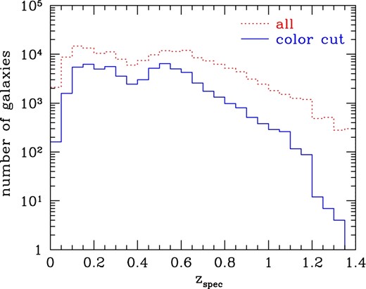
Number distribution of spectroscopic galaxies in the HSC Wide Survey as a function of spectroscopic redshift. The dotted line shows the distribution for all the spectroscopic galaxies. The solid line shows the distribution after the color cuts to select red-sequence galaxies (see the text for details). (Color online)

Open in new tabDownload slide

Fig. 2.

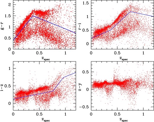
Colors of spectroscopic galaxies as a function of redshift. For illustrative purpose, we plot a subsample of only 5% of all the spectroscopic galaxies. We show g − r (upper left), r − i (upper right), i − z (lower left), and z − y (lower right). Solid lines show our color cuts defined by equations (1), (2), and (4). (Color online)

Open in new tabDownload slide

2.3 Updates of the CAMIRA algorithm

The detailed methodology of the CAMIRA algorithm was presented in Oguri (2014). In short, it fits all photometric galaxies with an SPS model of Bruzual and Charlot (2003) to compute likelihoods of them being red-sequence galaxies as a function of redshift. The model is calibrated using spectroscopic galaxies, which are used to derive residual colors of SPS model fitting as a function of wavelength and redshift (see also below). Using the likelihoods we define a non-integer “number parameter” for each galaxy as a function of redshift, such that the sum of number parameters reduces to richness. Using the number parameter, the three-dimensional richness map is constructed to locate cluster candidates from peaks in the richness map. In CAMIRA, richness describes the number of red member galaxies with stellar masses M_* ≳ 10^10.2 M_⊙ and within a circular aperture with a radius R ≲ 1 h⁻¹ Mpc in physical units. In fact, we use smooth filters for stellar masses, F_M(M_*) ∝ exp [−(M_*/10¹³ M_⊙)⁴ − (10^10.2 M_⊙/M_*)⁴], and for spatial distributions, F_R(R)∝Γ[4, (R/R₀)²] − (R/R₀)⁴exp [−(R/R₀)²] with R₀ = 0.8 h⁻¹ Mpc, to compute richness. The spatial filter is a compensated filter such that the background level is automatically subtracted in deriving richness. We then identify a brightest cluster galaxy (BCG) for each cluster candidate by selecting a high stellar mass galaxy near the richness peak, and refine richness, cluster photometric redshift, and the BCG, iteratively. Interested readers are referred to Oguri (2014) for more information.

3 Cluster catalog

3.1 Basic characteristics

We construct an HSC Wide S16A cluster catalog in the redshift range 0.1 < z_cl < 1.1, where z_cl denotes photometric redshifts of clusters. Cluster photometric redshifts are computed in the course of CAMIRA cluster finding by combining photometric redshifts of high-confidence cluster member galaxies (see Oguri 2014). The upper limit of the redshift comes mainly from the lack of spectroscopic galaxies for the calibration, but it is also due to the limited wavelength coverage. The lower limit of the redshift is because large angular sizes of low-redshift clusters make cluster-finding challenging, and member galaxies also tend to be too bright in HSC images. We select clusters with the mask-corrected richness |$\skew7\hat{N}_{\rm mem}$| (see Oguri 2014, for the definition) higher than 15. The catalog contains 1921 clusters.

In Oguri (2014), the richness |$\skew7\hat{N}_{\rm mem}$| is further corrected for the incompleteness of detections of member galaxies. This was particularly important for SDSS, in which our member galaxy selection (corresponding to L ≳ 0.2 L_*) was incomplete at z ≳ 0.3 due to the shallow depth of the SDSS images. In contrast, the HSC Wide Survey is deep enough to detect almost all member galaxies used for our cluster-finding (including the non-full-depth area we use in this paper), which again corresponds to L ≳ 0.2 L_*, even at z ∼ 1.1. Therefore in this paper we do not apply any richness correction due to member galaxy incompleteness (i.e., |$\skew7\hat{N}_{\rm cor}=\skew7\hat{N}_{\rm mem}$| in the notation of Oguri 2014). We show the spatial distribution of the HSC Wide S16A clusters in figure 3, and the distribution in the richness–redshift plane in figure 4. The area of the cluster search region of HSC Wide S16A is estimated to be ∼232 deg². The area is larger than that of the full-color and full-depth region of 174 deg² for the HSC Wide S16A dataset because we use the region that does not reach full depth, as described in subsection 2.1. We show HSC images of the richest clusters in several different redshift ranges in figure 5.

Fig. 3.

Spatial distribution of clusters. Filled points show the positions of HSC Wide S16A clusters presented in this paper. The planned footprint of the entire HSC Wide Survey is the region enclosed by dotted lines. We also show the spatial distribution of X-ray clusters used in section 5 with crosses. (Color online)

Open in new tabDownload slide

Fig. 4.

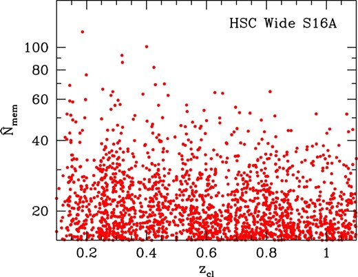
Distribution of clusters in the richness–redshift plane. The cluster catalog is constructed in the redshift range 0.1 < z_cl < 1.1 and the richness range |$\skew7\hat{N}_{\rm mem}>15$|⁠. (Color online)

Open in new tabDownload slide

Fig. 5.

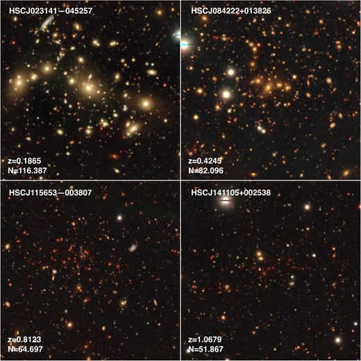
HSC grz-band color composite images of the richest clusters at different redshifts in the HSC Wide S16A cluster catalog. The cluster photometric redshift z = z_cl and richness |$N=\skew7\hat{N}_{\rm mem}$| are indicated in each panel. The size of each panel, which is centered at the BCG identified by the CAMIRA algorithm, is approximately 3|${^{\prime}_{.}}$|7 × 3|${^{\prime}_{.}}$|7. North is up and east is left. (Color online)

Open in new tabDownload slide

3.2 Number density of clusters

One way to infer the mass of a cluster catalog is to compare its number density with the number density of halos for a given cosmological model (e.g., Jimeno et al. 2017). We show the comoving number density of HSC Wide S16A clusters as a function of redshift in figure 6. The number density declines slowly with increasing redshift, which is consistent with the DES Science Verification (SV) data redMaPPer cluster catalog (Rykoff et al. 2016) and implies that the redshift evolution of the mass threshold is not strong. In order to check this point further, we compute the predicted number densities of halos with constant mass threshold using the halo mass function of Tinker et al. (2008). Here we adopt the mean overdensity mass M_200m which is defined as the mass enclosed within a sphere of radius r_200m within which the mean density is 200 times the mean matter density of the Universe. The comparison shown in figure 6 suggests that our richness threshold of |$\skew7\hat{N}_{\rm mem}>15$| roughly corresponds to the mass threshold of M_200m ≳ 10¹⁴ h⁻¹ M_⊙.

Fig. 6.

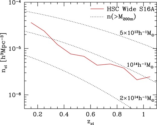
Comoving number density of HSC Wide S16A clusters as a function of cluster redshift (solid). The Poisson error is sufficiently small, ∼10% in each bin. Dotted lines show the predicted number densities of halos with masses M_200m > 5 × 10¹³ h⁻¹ M_⊙ (top), 10¹⁴ h⁻¹ M_⊙ (middle), and 2 × 10¹⁴ h⁻¹ M_⊙ (bottom), which are computed using a halo mass function of Tinker et al. (2008). (Color online)

Open in new tabDownload slide

3.3 Performance of photometric redshifts

Photometric redshifts of clusters, z_cl, are derived in the course of cluster finding (see Oguri 2014). In order to check the accuracy of cluster photometric redshifts, we cross-match the HSC Wide S16A cluster catalog with the spectroscopic galaxy catalog (subsection 2.2). We find that BCGs of 843 clusters have spectroscopic redshifts, z_BCG, spec. Figure 7 compares z_cl and z_BCG, spec, which clearly shows that cluster photometric redshifts are quite accurate for the whole redshift range. To quantify the accuracy of cluster photometric redshifts, we compute the residual (z_cl − z_BCG, spec)/(1 + z_BCG, spec) for all the clusters and define the bias δ_z and scatter σ_z by the average and standard deviation of the residual with 4σ clipping. We then define the outlier rate f_out as the fraction of galaxies that are removed by the 4σ clipping. Using all the galaxies, we find the bias δ_z = −0.0013, the scatter σ_z = 0.0081, and the outlier rate f_out = 0.017. In figure 7 we also show the bias δ_z and scatter σ_z as a function of redshift, finding that the bias is |δ_z| < 0.005 and the scatter is σ_z < 0.01 for most of the redshift range. This performance of cluster photometric redshifts is comparable to that of SDSS redMaPPer and CAMIRA clusters (Rykoff et al. 2014; Oguri 2014) and better than that of DES SV redMaPPer clusters (Rykoff et al. 2016). We note that the availability of a large sample of spectroscopic galaxies from SDSS and other spectroscopic surveys (see subsection 2.2) is an advantage of the HSC Survey over DES. However, as is clear from figure 7, there are not many spectroscopic galaxies at z ≳ 0.8, which suggests the importance of spectroscopic follow-up observations of those high-redshift clusters, to test their reliability further.

Fig. 7.

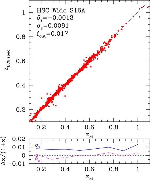
Upper: Comparison between cluster photometric redshifts z_cl and spectroscopic redshifts of BCGs z_BCG,spec. Lower: Bias δ_z (dashed) and scatter σ_z (solid) of the residual (z_cl − z_BCG,spec)/(1 + z_BCG, spec) as a function of redshift. (Color online)

Open in new tabDownload slide

4 Comparison with SDSS

Since the HSC data is much deeper than SDSS, it is expected that we can identify cluster member galaxies more reliably in HSC down to the stellar mass limit for the richness calculation, ∼10^10.2M_*, which roughly corresponds to the luminosity range of L ≳ 0.2L_* recommended in Rykoff et al. (2012). Due to the shallowness of the SDSS data, in Oguri (2014) we applied a richness correction factor |$f_N(z)=\skew7\hat{N}_{\rm mem}/\skew7\hat{N}_{\rm cor}$| to account for the incompleteness of member galaxy detections. In contrast, as discussed in subsection 3.1, in HSC we do not apply any correction for the member galaxy incompleteness simply because HSC data are deep enough to detect all the member galaxies of interest out to z ∼ 1.1. Thus we compare the richness in SDSS and HSC to check the accuracy of the incompleteness correction.

We cross-match the CAMIRA SDSS catalog with the HSC Wide S16A catalog. Our matching criterion is that clusters have a physical transverse distance within 1 h⁻¹ Mpc and a difference in cluster photometric redshifts that is smaller than 0.1. For the SDSS cluster catalog, we use an updated (v1.2) CAMIRA SDSS cluster catalog which slightly differs from the cluster catalog published in Oguri (2014). The updated CAMIRA SDSS catalog adopts the new centering parameters described in subsection 2.3, and contains 83735 clusters in the redshift range 0.1 < z_cl < 0.6 and with corrected richness |$\skew7\hat{N}_{\rm cor}>20$|⁠.¹

In figure 8, we compare the richness from HSC with the incompleteness-corrected richness from SDSS as a function of cluster redshift. While at low redshift these richness agree with each other, at higher redshift (z ≳ 0.3), where the richness correction is applied to SDSS richness, we find a systematic offset between these two richnesses, such that the richness in HSC is systematically lower than the richness in SDSS. This comparison suggests a possible systematic bias in the incompleteness correction in the CAMIRA SDSS cluster catalog, and hence highlights the importance of using deep data to detect sufficiently faint cluster members for optical cluster finding. The deep photometric data are also important for studying the redshift evolution of the luminosity function of cluster member galaxies.

Fig. 8.

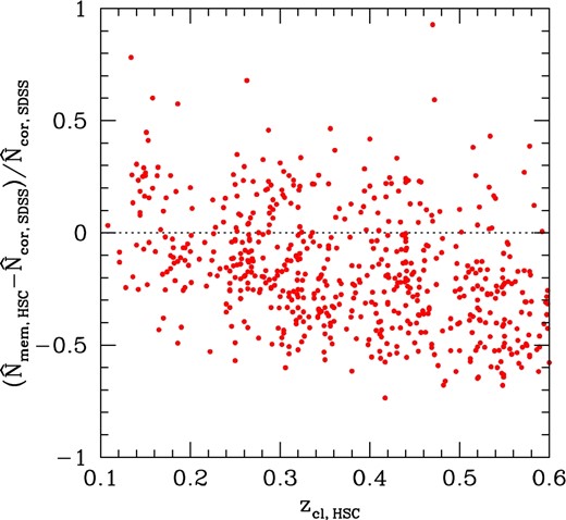
Comparison of the CAMIRA richness in HSC, |$\skew7\hat{N}_{\rm mem,HSC}$|⁠, with the incompleteness-corrected CAMIRA richness in SDSS, |$\skew7\hat{N}_{\rm cor, SDSS}$|⁠. The fractional difference of these two richness is plotted as a function of cluster redshift from HSC, z_{cl, HSC}. (Color online)

Open in new tabDownload slide

5 Comparison with X-ray cluster catalogs

5.1 X-ray catalogs

The footprint of the HSC Wide S16A cluster catalog has a large overlap with two large-area X-ray surveys, the XMM Large Scale Structure survey (XMM-LSS: Pierre et al. 2004) and the XXL survey (Pierre et al. 2016). We adopt a sample of 52 X-ray bright clusters selected from the 11 deg² XMM-LSS survey region presented in Clerc et al. (2014), and also a sample of 51 X-ray bright clusters from the ∼25 deg² XXL North survey region presented in Pacaud et al. (2016) and Giles et al. (2016). For both cluster catalogs we use X-ray centroids, redshifts from the spectroscopy of member galaxies, X-ray temperatures T_X, and rest-frame [0.5–2] keV luminosities within r_{500, MT}, L_{X, 500}, where r_{500, MT} is the radius within which the mean matter density of the cluster becomes 500 times the critical density of the Universe at the cluster redshift, with the corresponding mass M₅₀₀ estimated from a mass–temperature relation. In the XXL survey, T_X values are computed within a fixed aperture of 300 kpc. These two cluster catalogs have some overlap, and in this paper we use values from the XXL catalog when a cluster is included on both the XXL and XMM-LSS catalogs, because the XXL survey is an extension of the XMM-LSS survey. In addition, we remove four XXL cluster located at Dec < −6.6 as the HSC Wide S16A cluster catalog does not cover that area (see figure 3).

By combining these two X-ray cluster catalogs, we construct a sample of 77 X-ray bright clusters which are used for characterizing the HSC Wide S16A cluster catalog. The spatial distribution of these X-ray clusters is shown in figure 3.

5.2 Correlation of richness with X-ray properties

The comparison between the richness and X-ray properties such as the luminosity L_{X, 500} and temperature T_X is useful. Because X-ray properties are more tightly correlated with cluster masses (but see also Andreon & Hurn 2010; Andreon 2015), the correlation of richness with X-ray properties is often used as a proxy for the tightness of the correlation between the richness and the cluster mass (e.g., Rykoff et al. 2012; Rozo & Rykoff 2014; Oguri 2014; Wen & Han 2015).

We cross-match the HSC Wide S16A cluster catalog with the X-ray cluster catalog constructed in subsection 5.1. Again, we use a simple matching criterion; clusters that have a physical transverse distance of within 1 h⁻¹ Mpc and a redshift difference smaller than 0.1 are matched. When there are several matching candidates, we adopt clusters with the smallest transverse separation. Among the 77 X-ray bright clusters from XXL and XMM-LSS, 50 clusters are found to have counterparts in the HSC Wide S16A catalog. Some of the X-ray clusters have no counterpart in the HSC cluster catalog simply because their redshifts fall outside the redshift range of the HSC Wide S16A catalog (i.e., z < 0.1 or z > 1.1). There are other X-ray clusters that fall within the redshift range of the CAMIRA catalog but have no counterpart, which are used to estimate the completeness of the HSC cluster catalog (see subsection 5.3).

Fig. 9.

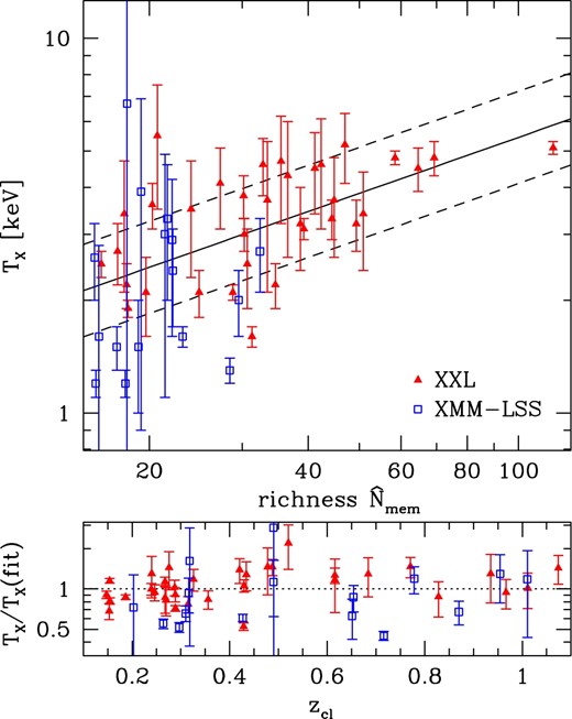
Comparison between richness |$\skew7\hat{N}_{\rm mem}$| and X-ray temperature T_X for XXL (filled triangles) and XMM-LSS (open squares) clusters. The solid and dashed lines show the best-fitting richness–temperature relation and the range of ±1σ intrinsic scatter. The lower panel shows the residual of fitting as a function of redshift. (Color online)

Open in new tabDownload slide

Fig. 10.

Same as figure 9, except that the comparison between richness |$\skew7\hat{N}_{\rm mem}$| and evolution-corrected X-ray luminosity [E(z)]⁻¹L_X,500 is shown. (Color online)

Open in new tabDownload slide

The residual of fitting as a function of redshift shown in figure 10 indicates a clear trend with redshift. This may suggest a redshift evolution stronger than the self-similar prediction, i.e., γ_LT > 1 (see also Giles et al. 2016), although it must be partly due to the Malmquist bias. This is because the X-ray cluster sample is a flux-limited sample and X-ray luminosities are more directly related to X-ray fluxes. The idea is supported by the fact that XMM-LSS clusters, which have the lower X-ray flux limit, tend to have lower luminosities than those of XXL clusters at all redshift range. Hence in order to derive the intrinsic scaling relation we need to take account of flux limits of these X-ray surveys, which we leave for future work.

5.3 Completeness estimation

In addition to using mocks (see section 6), we estimate the completeness of the HSC Wide S16A catalog using the X-ray cluster catalog. Here, we adopt a simple approach to estimate the completeness by the fraction of X-ray clusters with optical counterparts to all X-ray clusters. Given an ambiguity of matching between HSC and X-ray clusters, the completeness presented here should be interpreted with caution. We derive the completeness as a function of X-ray temperature threshold; for a given T_X, we use all X-ray clusters above that T_X to derive the completeness. We also restrict the redshift range of the X-ray clusters to 0.1 < z < 1.1 for the completeness estimation.

Figure 11 plots the estimated completeness as a function of X-ray temperature threshold. We find that the completeness is generally high, ∼0.8–0.9. There are a couple of X-ray clusters with relatively high X-ray temperatures, T_X ∼ 5 keV, which do not have counterparts in the HSC cluster catalog. We find that these X-ray clusters have companion X-ray clusters separated by ∼8΄ at similar redshifts. For example, one of them corresponds to a member of a supercluster of galaxies at z = 0.43 (Pompei et al. 2016). Since the CAMIRA algorithm adopts a compensated spatial filter for creating a richness map (Oguri 2014), detections of companion clusters near massive clusters tend to be suppressed, as also noted in Miyazaki et al. (2015). The current analysis of completeness is limited by the small number of X-ray clusters in the sample, and an extended analysis using a larger sample of X-ray clusters is useful for quantifying the impact of paired clusters on the completeness.

Fig. 11.

Completeness of HSC Wide S16A clusters, which is estimated using X-ray clusters. The completeness is defined by the fraction of X-ray clusters that match the HSC cluster catalog to all X-ray clusters. The completeness is estimated as a function of X-ray temperature threshold (i.e., for each T_X all X-ray clusters with >T_X are used to derive the completeness). (Color online)

Open in new tabDownload slide

5.4 Positional offset distribution

It has been known that optical cluster finders often misidentify centers of clusters. This mis-centering effect is important for applications of optically-selected clusters, such as weak lensing analysis. Mis-centering of optically-selected clusters has indeed been studied with various approaches, including offsets between optical and X-ray cluster centers (e.g., Lin et al. 2004; Mahdavi et al. 2013; Rozo & Rykoff 2014; Oguri 2014; Rykoff et al. 2016), offsets between optical and SZ cluster centers (e.g., Song et al. 2012; Sehgal et al. 2013; Sifón et al. 2013; Saro et al. 2015), and weak lensing (e.g., Oguri et al. 2010; George et al. 2012; Oguri 2014; Ford et al. 2014, 2015; Viola et al. 2015; van Uitert et al. 2016; Miyatake et al. 2016). In this paper we use offsets between HSC Wide S16A clusters, the centers of which are defined by the locations of BCGs identified by the CAMIRA algorithm (see Oguri 2014), and the X-ray clusters from XXL and XMM-LSS to study the mis-centering effect.

Fig. 12.

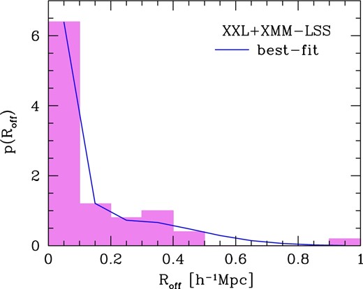
Distribution of positional offset between HSC Wide S16A clusters and X-ray clusters, which is derived using 50 X-ray clusters from XXL and XMM-LSS surveys that match the HSC cluster catalog. The offsets R_off are defined by physical transverse distances between HSC and X-ray cluster centers. The solid line shows the best-fitting model assuming the functional form of equation (9). (Color online)

Open in new tabDownload slide

We check the possible richness-dependence of the offset distribution by dividing the cluster catalog into two richness bins, |$\skew7\hat{N}_{\rm mem}<30$| and |$\skew7\hat{N}_{\rm mem}>30$|⁠, and repeating the analysis above. Given the smaller number of X-ray clusters in each richness bin, we fix σ₁ and σ₂ to the best-fitting values obtained from the analysis of the full sample, and fit only f_cen. We find that f_cen = 0.66 ± 0.10 for |$\skew7\hat{N}_{\rm mem}<30$|⁠, and f_cen = 0.71 ± 0.12 for |$\skew7\hat{N}_{\rm mem}>30$|⁠, which indicates that there is no strong dependence of the offset distribution on richness.

6 Analysis of mock galaxy samples

6.1 Construction of mock galaxy samples

We create mock galaxy samples specifically designed for testing cluster-finding algorithms. Since accurate galaxy colors are crucial for this purpose, we use colors of true observed galaxies in the HSC Survey. We use the HSC galaxy catalog in the COSMOS (Scoville et al. 2007) field for the field galaxy population, and use CAMIRA clusters in HSC Wide S16A to select cluster member galaxies. N-body simulations are used to produce realistic distributions of halo masses and redshifts. Thus our mock galaxy catalogs use realistic cluster distributions, and also contain gaps and holes in the spatial distribution of galaxies due to bright stars and bad columns, which allow realistic characterization of completeness and purity. We provide a detailed description of our mock galaxy samples in appendix 3.

We note that we need to make assumptions on the input richness–mass relation, the red galaxy fraction, and their redshift evolution in order to create these mock galaxy samples, which may not necessarily be correct. While quantitative results such as the scatter in the observed richness–mass relation and the completeness as a function of halo masses depend on these assumptions, we expect that the qualitative behavior of the completeness and purity estimated from these mocks is not very sensitive to these assumptions.

6.2 Analysis results

We run the CAMIRA algorithm on the mock galaxy samples using the same set-up as the one used to create the HSC Wide S16A catalog. We then cross-match CAMIRA cluster catalogs of the mocks with input halo catalogs. We use the matching criterion of the physical transverse distance being smaller than 1 h⁻¹ Mpc and the difference between the halo redshift and the cluster photometric redshift being smaller than 0.1. Given the limited range of the redshift and halo mass of our mock galaxy samples (see appendix 3), we also restrict the redshift range of halos to 0.3 < z_halo < 1.0 and the mass range to M_200c > 2 × 10¹³ h⁻¹ M_⊙ for the cross-matching. We record all clusters and halos that fall within the same redshift range but fail to match, which are used to estimate completeness and purity below. We analyze 90 realizations of the COSMOS-size mock galaxy samples, leading to a total area of ∼144 deg².

Figure 13 shows the result of matching. As expected, we can clearly see a positive correlation between halo masses and richness. We find that most of the CAMIRA clusters in the mocks have counterparts in the halo catalog except for the very low richness end, which indicates that the purity of the CAMIRA cluster catalog, which is defined by the fraction of CAMIRA clusters that corresponds to real massive halos, is high; >0.95 down to the richness limit of |$\skew7\hat{N}_{\rm mem}=15$|⁠. On the other hand, figure 13 indicates that there are halos up to ∼10¹⁴ h⁻¹ M_⊙ that are not detected by the CAMIRA algorithm, which implies that the completeness, which is defined by the fraction of halos that are correctly identified by the CAMIRA algorithm, requires careful study.

Fig. 13.

Comparison of cluster richness |$\skew7\hat{N}_{\rm mem}$| and halo mass M_200c from the analysis of mock galaxy catalogs (see subsection 6.1 for the description). For illustrative purpose, we assign |$\skew7\hat{N}_{\rm mem}=12$| for halos without any counterpart in the cluster catalog, and M_200c = 1.5 × 10¹³ h⁻¹ M_⊙ for clusters without any counterpart in the halo catalog. The dashed line shows a power-law fit to 〈log M|N〉 using the matching result with |$\skew7\hat{N}_{\rm mem}>20$| [see equation (11)]. In the upper and right-hand panels, we also show the histograms of matched (solid) and unmatched (dashed) clusters/halos. (Color online)

Open in new tabDownload slide

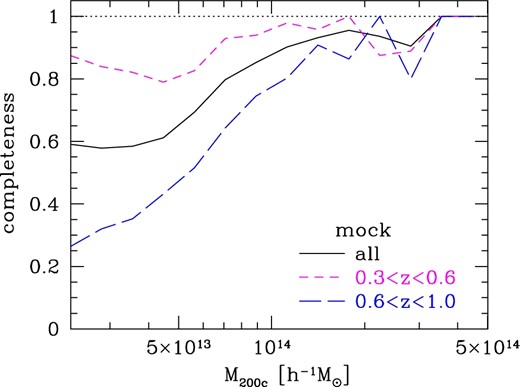
Figure 14 shows the completeness defined by equation (16). Here we adopt N_lim = 15, although the result is insensitive to the specific choice of N_lim, as expected. We note that, for N_lim = 15, the correction factor S(M) is very close to unity down to M_200c ∼ 10¹⁴ h⁻¹ M_⊙ and decreases to ∼0.5 at M_200c ∼ 3 × 10¹³ h⁻¹ M_⊙, and hence the correction of the completeness due to S(M) is relatively minor. We find that the completeness after the N_lim correction is reasonably high (>0.9) at the high-mass end, M_200c ≳ 10¹⁴ h⁻¹ M_⊙, and decreases below 10¹⁴ h⁻¹ M_⊙. This result is also broadly consistent with the completeness estimated from X-ray clusters shown in figure 11. A possible explanation of decreasing completeness at the low-mass end is that the scatter in the richness–mass relation increases rapidly toward lower richness, due to the larger Poisson noise of the number of cluster member galaxies and more significant contribution of background fluctuations to the richness that enhances the scatter. In either case, the high completeness at high cluster masses is encouraging from the viewpoint of using massive optically-selected clusters as a cosmological probe.

Fig. 14.

Completeness estimated from the analysis of mock galaxy catalogs as a function of halo mass M_200c. The completeness is defined by equation (16). The solid line shows the completeness using all halos. Short-dashed and long-dashed lines indicate the completeness for subsamples of halos at 0.3 < z < 0.6 and 0.6 < z < 1.0, respectively. (Color online)

Open in new tabDownload slide

Fig. 15.

Comparison of cluster photometric redshifts z_cl between HSC Wide S16A cluster catalogs with and without the bright-star mask. (Color online)

Open in new tabDownload slide

Fig. 16.

Comparison of richness |$\skew7\hat{N}_{\rm mem}$| between HSC Wide S16A cluster catalogs with and without the bright-star mask. (Color online)

Open in new tabDownload slide

It is possible that the completeness changes with redshift. To check the possible redshift dependence, we divide the mock halo sample into two redshift bins with 0.3 < z < 0.6 and 0.6 < z < 1.0, and derive completeness for both the subsamples. The result shown in figure 14 indicates that the completeness indeed depends on the redshift. For the low-redshift halos, the completeness remains high down to ∼8 × 10¹³ h⁻¹ M_⊙, whereas for high-redshift halos the completeness starts to drop at higher masses. Decreasing completeness with increasing redshift for a fixed halo mass may be partly due to a decreasing red galaxy fraction, which is taken into account in the mock galaxy catalog construction (see appendix 3). In both redshift bins the completeness is close to unity above ∼1.5 × 10¹⁴ h⁻¹ M_⊙. This redshift evolution of the completeness should also be taken into account for careful statistical studies of CAMIRA clusters.

Again, we emphasize that our quantitative results from the mock catalog depending on input models, such as cosmological parameters and mass–richness relations for populating galaxies in halos, which can differ from true values. For example, the redshift evolution of the completeness discussed above depends crucially on the redshift evolution of the input mass–richness relation and the input redshift evolution of the red fraction in clusters (see appendix 3). In particular, we note that our current mock catalog appears to overestimate richness, in the sense that the number density of CAMIRA-detected clusters in the mock as a function of richness is a factor of ∼4 higher than in observations, which suggests room for improvement of the mock. Nevertheless, the mock result should still be useful for understanding qualitative behavior of the completeness and purity of the CAMIRA algorithm, and both the mock catalog analysis presented here and the comparison with other (such as X-ray) cluster catalogs, as presented in section 5, are important for characterizing the CAMIRA cluster catalog.

7 Summary

We have presented a new optically-selected cluster catalog from the HSC Survey. Using the HSC Wide S16A dataset covering ∼232 deg², we have constructed a sample of 1921 clusters at redshift 0.1 < z_cl < 1.1 and with richness |$\skew7\hat{N}_{\rm mem}>15$|⁠. Based on the number density, we infer that the rough mass limit of the cluster sample is M_200m ≳ 10¹⁴ h⁻¹ M_⊙. We have found that cluster redshifts are accurate with bias δ_z < 0.005 and scatter σ_z < 0.01 for most of the redshift range. The photometric redshift accuracy is comparable to that of optically-selected clusters in SDSS, but HSC clusters extend to much higher redshifts. We have also compared the HSC Wide S16A cluster catalog with X-ray clusters from XXL and XMM-LSS surveys, finding tight correlations between richness and X-ray properties. In addition, we have derived the distribution of positional offsets of cluster centers using the X-ray clusters and found that the fraction of well-centered clusters is ∼0.7, with no significant dependence on richness. We have analyzed mock galaxy catalogs to study the completeness and purity. We have found a high purity, and also a high completeness for halos with masses above ∼10¹⁴ h⁻¹ M_⊙. The completeness depends on redshift such that completeness for lower-mass halos is higher at lower redshift.

This work presents the first cluster catalog from the HSC Survey, and demonstrates the power of the HSC Survey for studies of high-redshift clusters. The exquisite depth of the HSC Survey allows us to detect almost all cluster member galaxies above M_* ∼ 10^10.2 M_⊙ even at z ∼ 1.1, and hence allows a reliable cluster search at such high redshifts. For instance, by extrapolating the result in this paper, we expect to construct a large catalog of ∼1000 clusters with richness |$\skew7\hat{N}_{\rm mem}>20$| at z ∼ 1 from the final HSC Wide Survey dataset covering ∼1400 deg². We plan to calibrate cluster masses using a stacked weak lensing technique, as well as careful comparisons with X-ray and SZ cluster catalogs, including an extended XXL X-ray cluster catalog and SZ clusters from ACTPol (Niemack et al. 2010).

Acknowledgements

We thank Cristóbal Sifón for useful comments, and an anonymous referee for useful suggestions. This work is supported in part by World Premier International Research Center Initiative (WPI Initiative), MEXT, Japan, and JSPS KAKENHI Grant Number 26800093. This work is in part supported by MEXT Grant-in-Aid for Scientific Research on Innovative Areas (No. 15H05887, 15H05892, 15H05893). YTL acknowledges support from the Ministry of Science and Technology grants MOST 104-2112-M-001-047 and MOST 105-2112-M-001-028-MY3. HM is supported by the Jet Propulsion Laboratory, California Institute of Technology, under a contract with the National Aeronautics and Space Administration.

The Hyper Suprime-Cam (HSC) collaboration includes the astronomical communities of Japan, Taiwan, and Princeton University. The HSC instrumentation and software were developed by the National Astronomical Observatory of Japan (NAOJ), the Kavli Institute for the Physics and Mathematics of the Universe (Kavli IPMU), the University of Tokyo, the High Energy Accelerator Research Organization (KEK), the Academia Sinica Institute for Astronomy and Astrophysics in Taiwan (ASIAA), and Princeton University. Funding was contributed by the FIRST program from Japanese Cabinet Office, the Ministry of Education, Culture, Sports, Science and Technology (MEXT), the Japan Society for the Promotion of Science (JSPS), Japan Science and Technology Agency (JST), the Toray Science Foundation, NAOJ, Kavli IPMU, KEK, ASIAA, and Princeton University.

The Pan-STARRS1 Surveys (PS1) have been made possible through contributions of the Institute for Astronomy, the University of Hawaii, the Pan-STARRS Project Office, the Max-Planck Society and its participating institutes, the Max Planck Institute for Astronomy, Heidelberg and the Max Planck Institute for Extraterrestrial Physics, Garching, The Johns Hopkins University, Durham University, the University of Edinburgh, Queen’s University Belfast, the Harvard-Smithsonian Center for Astrophysics, the Las Cumbres Observatory Global Telescope Network Incorporated, the National Central University of Taiwan, the Space Telescope Science Institute, the National Aeronautics and Space Administration under Grant No. NNX08AR22G issued through the Planetary Science Division of the NASA Science Mission Directorate, the National Science Foundation under Grant No. AST-1238877, the University of Maryland, and Eotvos Lorand University (ELTE).

This paper makes use of software developed for the Large Synoptic Survey Telescope. We thank the LSST Project for making their code available as free software at http://dm.lsst.org.

Based (in part) on data collected at the Subaru Telescope and retrieved from the HSC data archive system, which is operated by the Subaru Telescope and Astronomy Data Center at National Astronomical Observatory of Japan.

Appendix 1. Cluster catalogs

We construct three cluster catalogs from the HSC S16A data. The first catalog is from the Wide region without applying a bright-star mask. This catalog is used in the analysis throughout the paper. The second catalog is also from the Wide region, but with a bright-star mask applied. The bright-star mask removes objects near bright stars, and the current mask is designed conservatively such that it removes nearly ∼10% of objects. The current cluster catalog with the star mask suffers from the effect of masking bright galaxies, which is discussed in appendix 2. The third catalog is from the Deep region covering ∼25 deg². Even though the Deep data are deeper than the Wide data, we use the same selection criteria for constructing an input galaxy catalog, including the conservative z-band magnitude limit of z < 24. These catalogs are shown in Supplementary Tables 1, 2, and 3.

Appendix 2. Effect of the bright-star mask on cluster finding

In addition to overly conservative sizes of mask regions, a known issue of the current version of the bright-star mask is that it also masks bright nearby galaxies (Aihara et al. 2018). This is because a bright object catalog from the Naval Observatory Merged Astrometric Dataset (NOMAD: Zacharias et al. 2005), which we use to select mask regions, often misinterprets nearby bright galaxies as stars. We check the impact of masking bright galaxies on cluster-finding by comparing cluster catalogs with and without star masks.

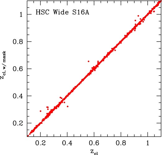
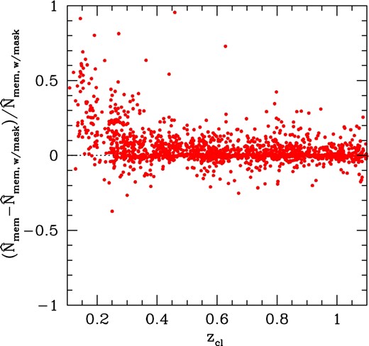
We match HSC Wide S16A cluster catalogs with and without the bright-star mask in the same manner as in section 4. The comparison of cluster photometric redshifts shown in figure 15 indicates that photometric redshifts agree well between these two cluster catalogs. In contrast, the comparison of richness in figure 16 shows a clear bias at low redshifts, z ≲ 0.4, such that richness in the cluster catalog with the bright-star mask is systematically lower than in the cluster catalog without the bright-star mask. We find that this is due to masking of bright galaxies as mentioned above, which masks red member galaxies near BCGs, as well as BCGs themselves, leading to smaller richness estimates for those clusters. Therefore, for any cluster studies that involve low-redshift clusters, we recommend against the use of the cluster catalog with the bright-star mask. For studies of high-redshift (z ≳ 0.4) clusters, however, the effect of masking bright galaxies is negligible and we expect we can safely use the cluster catalog with a bright-star mask.

As discussed in Aihara et al. (2018), we are working on revising the bright-star mask, and we expect that this issue will be resolved in future versions of HSC CAMIRA cluster catalogs.

Appendix 3. Description of the mock galaxy catalog

The set of mock galaxy catalogs we use for testing the cluster-finding algorithm is produced by combining a “field” galaxy population with a “cluster” galaxy population. In a nutshell, the “field” population is generated from well-studied extragalactic fields with rich multiwavelength data (particularly in X-rays), so that galaxies associated with massive galactic systems such as clusters and groups can be removed (leaving only the field galaxies). On the other hand, the “cluster” population is obtained by populating dark matter halos with galaxies from real, observed clusters. Below we briefly describe how each of these is produced.

For the field galaxy catalog, we use the HSC Subaru Strategic Program observation of the COSMOS (Scoville et al. 2007) field as the parent sample. More specifically, we adopt the Wide-layer depth grizy-band photometry of the Ultradeep-layer observation. We further remove galaxies that are likely associated with known structures in the COSMOS field, such as galaxy groups and clusters, by excluding ∼4000 galaxies that have membership probability P_mem > 0.5 according to the galaxy group catalog of George et al. (2011).

As for the actual cluster member galaxy data used in this procedure, we have selected the top five richest clusters detected by CAMIRA in each of the redshift bins from z = 0.3 to z = 1.0, with bin width of 0.1. For each of these real clusters, we initially consider all galaxies lying within a projected distance of |$\tilde{R}_{\rm 200c}$|⁠. Here |$\tilde{R}_{\rm 200c}$| is a rough estimate of the true value for these massive clusters, obtained by taking an average of five of the richest mock clusters from the public Marenostrum Institut de Ciéncies de l'Espai (MICE) mock catalog (Carretero et al. 2015) selected in the same redshift range, over an area of 200 deg².² The subsequent treatment is different for red and blue galaxies. For the galaxies on the red sequence, we simply select the needed N_red galaxies, giving preference to the brighter galaxies, using simple red galaxy selections in the color–magnitude diagram. A caveat is that this procedure of populating red galaxies from brighter to fainter galaxies using the richest clusters may introduce bias in mock galaxy population, such as the overestimation of the bright end of the low-mass cluster luminosity functions, which is ignored here. For the blue galaxies, we use photometric redshifts (using Easy and Accurate Redshifts from Yale, EAZY: Brammer et al. 2008) derived from the HSC Survey data to facilitate the selection, taking into account the accuracy of the photometric redshift as a function of magnitude, and draw in random N_blue galaxies from the blue cloud by giving higher priority to brighter galaxies. For a given halo in the lightcone, we select the real cluster that is closest in terms of both redshift and richness. To account for the fact that real clusters do not lie at the same redshifts of the halos, we use a passively-evolving stellar population model based on the Bruzual and Charlot (2003) model to shift the real galaxies either forward or backward in time with a typical magnitude shift of 0.03. Finally, while we keep the relative orientation of galaxies with respect to the cluster center (defined to be the location of the brightest cluster galaxy), we rescale the radial distance by the halo mass, assuming an NFW profile (Navarro et al. 1997) with the concentration parameter of c = 5. The value of the concentration parameter we adopted is a typical value for the dark matter distribution of halos with masses and redshifts of our interest (e.g., Gao et al. 2008).

In principle, we could include member galaxies in clusters selected by other means, such as X-rays or the SZ effect. For the current version of the mock, we have opted to use CAMIRA-selected clusters as these are detected over much larger areas than existing X-ray surveys, and thus represent currently the best-available massive cluster sample. As an exploratory example, we also attempt another set of mocks (hereafter referred to as the “test set”), which differs from our default set in the source of the input clusters. Instead of using the richest CAMIRA clusters, we resort to known X-ray clusters covered by the current HSC footprint that are also matched to the CAMIRA cluster catalog. As mentioned above, one important limitation for adopting the X-ray-selected clusters is that, due to the small area coverage in the X-ray surveys (only a small fraction of the HSC survey footprint has deep X-ray data for detecting clusters out to high redshifts), the clusters are typically much poorer than those used in our default mock set (see figure 17), which makes our galaxy selection process more vulnerable to contamination from foreground/background galaxies and may lead to lower completeness. In the future we should use X-ray or SZ-selected clusters in order to avoid any selection bias of optically-selected clusters which, by definition, contain prominent concentrations of red cluster member galaxies.

Fig. 17.

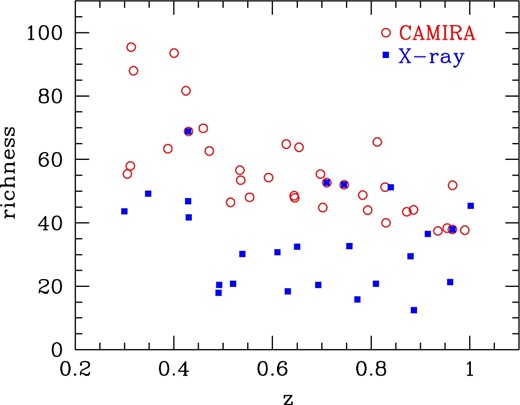
Comparison of the clusters used to “populate” the halos between our default set (open circles; 35 clusters) and the test set (filled square; 25 clusters). The default set uses richest CAMIRA clusters, while the test set employs those CAMIRA clusters that are also detected in the X-rays, which are mostly from the XXL and XMM Cluster Survey (XCS: Mehrtens et al. 2012). (Color online)

Open in new tabDownload slide

After all the halos in the lightcone patch have been populated with galaxies from real galactic systems (modulo shifts in redshift using passive evolution), we finally remove those galaxies lying in the gap and bright star regions seen in the field galaxy catalog mentioned above, and combine the resulting galaxy catalog with the field galaxy catalog. On average, on top of the ∼130000 galaxies in the field, we add about 7000 cluster galaxies. We show an example of the distribution of the mock galaxies in figure 18. We note that the spatial distribution of our mock galaxy sample contains several vertical stripes of gaps, which are not seen in most of the HSC Wide layer data. Since these stripes are expected to reduce the completeness estimated from these mock galaxy samples, we expect that our mock analysis results presented in section 6 are conservative.

Fig. 18.

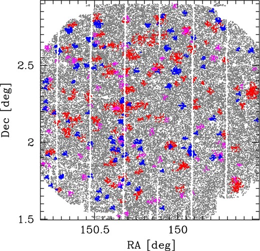
An example of our mock galaxy catalogs for testing cluster-finding algorithms. Small gray dots show the distribution of “field” galaxies, taken from real HSC observations. Red squares, magenta triangles, and blue circles show the distribution of “cluster” galaxies at redshift 0.3 < z < 0.6, 0.6 < z < 0.9, and 0.9 < z < 1.2, respectively. (Color online)

Open in new tabDownload slide

As our N-body lightcone covers an octant of the sky, we can extract many patches of the mock sky identical in geometry to the COSMOS field, and thus rapidly generate mock catalogs with areas of hundreds of square degrees or more, although the spatial distribution of the field galaxies would be repeated and discontinuous if all the patches are combined together. Furthermore, as the same set of large-scale structures in COSMOS are repeated in all the mocks, the effects of large-scale structure in cluster-finding may not be fully captured in this approach. We do note that halos found in filamentary structures surrounding massive halos are also populated with galaxies, and therefore in our mocks the projection effects from surrounding large-scale structures are accounted for to some degree. Finally, it should be emphasized that the way we create the cluster galaxies inevitably relies on several assumptions on the redshift evolution of the cluster galaxy population (e.g., the evolution of the halo occupation number and the red galaxy fraction), and thus our mocks should be regarded as a model, which still needs to be calibrated against detailed observations of distant clusters (e.g., Hennig et al. 2017). A proper way to obtain completeness and purity from our mocks is thus to generate sets of mocks that cover the ranges of plausible values of model parameters [e.g., c in equation (17), form and normalization of f_red], and marginalize over them.

Supporting Information

Supplementary data are available at PASJ online.

Supplementary Tables 1, 2, and 3.

Footnotes

References