


Abstract
We present the results from the Hitomi Soft Gamma-ray Detector (SGD) observation of the Crab nebula. The main part of SGD is a Compton camera, which in addition to being a spectrometer, is capable of measuring polarization of gamma-ray photons. The Crab nebula is one of the brightest X-ray/gamma-ray sources on the sky, and the only source from which polarized X-ray photons have been detected. SGD observed the Crab nebula during the initial test observation phase of Hitomi. We performed data analysis of the SGD observation, SGD background estimation, and SGD Monte Carlo simulations, and successfully detected polarized gamma-ray emission from the Crab nebula with only about 5 ks exposure time. The obtained polarization fraction of the phase-integrated Crab emission (sum of pulsar and nebula emissions) is (22.1% ± 10.6%), and the polarization angle is |${110{^{\circ}_{.}}7}$| +|${13{^{\circ}_{.}}2}$|/−|${13{^{\circ}_{.}}0}$| in the energy range of 60–160 keV (the errors correspond to the 1 σ deviation). The confidence level of the polarization detection was 99.3%. The polarization angle measured by SGD is about one sigma deviation with the projected spin axis of the pulsar, |${124{^{\circ}_{.}}0}$| ± |${0{^{\circ}_{.}}1}$|.
1 Introduction
In addition to spectral, temporal, and imaging information gleaned from observations of any astrophysical sources, polarization of electromagnetic emission from those sources provides the fourth handle on understanding the radiative processes involved. Historically, measurement of high radio polarization from celestial sources implicated synchrotron radiation as such a process, first suggested by Shklovsky (1970). Measurement of radio or optical polarization is relatively straightforward: first, it can be done from the Earth’s surface, and second, the instruments are relatively simple. Measurements in the X-ray band are more complicated: these have to be conducted from space, which constrains the instrument size, and, unlike, e.g., radio waves, X-rays are usually detected as particles and require large statistics to measure the polarization.
One of the brightest X-ray sources on the sky, with appreciable polarization measured in the radio and optical bands, is the Crab nebula. It has been detected by (probably) every orbiting X-ray astronomy mission (for a recent summary, see Hester 2008). It was thus expected that X-ray polarization should be detected as well, and in fact the first instrument sensitive to X-ray polarization, the OSO-8 mission, observed the Crab nebula and detected X-ray polarization (Weisskopf et al. 1978). The measurement, performed at 2.6 keV, measured polarization at roughly ∼20 ± 1% level. It was some 30 years later that the INTEGRAL mission observed the Crab nebula and detected significant polarization of its hard X-ray / soft γ-ray emission (Forot et al. 2008; Chauvin et al. 2013). Moreover, INTEGRAL teams reported gamma-ray polarization measurements from the black hole binary system Cygnus X-1
(Laurent at al. 2011; Jourdain et al. 2012; Rodriguez et al. 2015). However, interpretation of the measurements with INTEGRAL are not straightforward, because its instruments were not designed or calibrated for polarization measurements.
More recently, the Crab nebula was observed by the balloon-borne missions PoGOLite Pathfinder (Chauvin et al. 2016) and PoGO+ (Chauvin et al. 2017, 2018), with clear detection of soft γ-ray polarization in the ∼18–160 keV band, thus expanding the X-ray band where the Crab nebula emission shows polarization. PoGO+ is an instrument employing a plastic scintillator, with an effective area of 378 cm2 and optimized for polarization measurements of Compton scattering perpendicular to the incident direction, where the modulation factor of the azimuth scattering angle is high; the PoGO+ team reported a polarization of the phase-integrated Crab emission of 20.9% ± 5.0% with a polarization angle of |${131{^{\circ}_{.}}3}$| ± |${6{^{\circ}_{.}}8}$|, while in the off-pulse phase, it is |$17.4^{+8.6}_{-9.3}$|% with a polarization angle of 137° ± 15°.
The Japanese mission Hitomi (Takahashi et al. 2018), launched in 2016, included the Soft Gamma-ray Detector (SGD), an instrument sensitive in the 60–600 keV range, but also capable of measuring polarization (see Tajima et al. 2018) since it employs a Compton camera as a gamma-ray detector. The SGD was primarily designed as a spectrometer, but it was also optimized for polarization measurements (see, e.g., Tajima et al. 2010). For example, the Compton camera of the SGD is highly efficient for Compton scattering perpendicular to the incident photon direction and is symmetric with 90° rotation. Calibration and performance verification as a polarimeter had already been performed by using a polarized soft gamma-ray beam at SPring-8 (Katsuta et al. 2016). Hitomi observed the Crab nebula in the early phase of the mission. Since the goal of the observation reported here was to verify the performance of Hitomi’s instruments rather than to perform detailed scientific studies of the Crab nebula, the observation time was short. Even though this observation was conducted during orbits where the satellite passed through high-background orbital regions, including orbits crossing the South Atlantic Anomaly, the Crab nebula was still readily detected, as we report in subsequent sections. We discuss the data reduction and analysis in sections 2 and 3, the measurement of Crab’s polarization in section 4, compare our measurement to previous measurements in section 5, where we also discuss the implications on the modeling of the Crab nebula. We note that the Crab nebula observations with Hitomi’s Soft X-ray Spectrometer were published recently (Hitomi Collaboration 2018a), and observations with the Hard X-ray Imager are in preparation. Moreover, the data analysis of the Crab pulsar with Hitomi’s instruments have also been published (Hitomi Collaboration 2018b).
2 Crab observation with SGD
2.1 Instrument and data selection
The SGD was one of the instruments deployed on the Hitomi satellite (see Takahashi et al. 2018 for a detailed description of the Hitomi mission). The instrument was a collimated Si/CdTe Compton camera with a field of view of |${0{^{\circ}_{.}}6}$| × |${0{^{\circ}_{.}}6}$|, sensitive in the 60–600 keV band; for details of the SGD, see Tajima et al. (2018). The SGD Compton camera consisted of 32 layers of Si pixel sensors, where Compton scatterings take place primarily. Each layer of the Si sensor had a 16 × 16 array of 3.2 × 3.2 mm2 pixels with a thickness of 0.6 mm. In order to efficiently detect photons scattered in the Si sensor stack, it was surrounded on five sides by 0.75 mm-thick CdTe pixel sensors, where photo-absorptions take place primarily. In the forward direction, eight layers of CdTe sensors with a 16 × 16 array of 3.2 × 3.2 mm2 pixels were placed, while two layers of CdTe sensors with a 16 × 24 array of 3.2 × 3.2 mm2 pixels were placed on four sides of the Si sensor stack. For details of SGD Compton camera, see Watanabe et al. (2014). The SGD consisted of two detector units, SGD1 and SGD2, each containing three Compton cameras, named CC1, CC2, and CC3, respectively. These detectors were surrounded on five sides by an anti-coincidence detector containing a BGO scintillator. The observation of the Crab nebula with Hitomi was performed from 12:35 to 18:01 UT on 2016 March 25. This observation followed the start-up operations for the SGD, which were held from March 15 to March 24, and all the cameras of both SGD1 and SGD2 went into the nominal observation mode before the Crab nebula observation. However, just before the Crab nebula observation it was found that one channel in the CdTe detectors of SGD2 CC2 became noisy, and subsequently we set the voltage value of the high-voltage power supply for the CdTe sensors of the SGD2 CC2 to 0 V during the Crab nebula observation. Since CC3 shares the same high-voltage power supply as CC2, the CdTe sensors in CC3 were also disabled. Therefore, four of the six Compton cameras (SGD1 CC1, CC2, CC3, and SGD2 CC1) were operated in the nominal mode, which enabled the Compton event reconstruction.
Good time intervals (GTI) of the SGD during the Crab observation are listed in table 1. The intervals during the Earth occultation and South Atlantic Anomaly (SAA) passages are excluded. The total on-source duration was 8.6 ks. The exposure times of each Compton camera after dead-time corrections are listed in table 2. In the SGD1 Compton cameras, the dead-time-corrected exposure time can be derived from the number of “clean” pseudo events (Watanabe et al. 2014), which have no FBGO flag and no HITPATBGO flag. The pseudo events are events triggered by “pseudo triggers,” which are generated randomly in the Compton camera FPGA based on pseudorandom numbers calculated in the FPGA. The count rate of the pseudo triggers was set to be 2 Hz. The FBGO and HITPATBGO flags indicate the existence of anti-coincidence signals from the BGO shield. The pseudo events are processed in the same manner as usual triggers, and are discarded if the pseudo trigger is generated while a “real event” is inhibiting other triggers. Therefore, the dead-time fraction can be estimated by counting the number of pseudo events, and the dead-time by accidental hits in BGOs can also be estimated from the pseudo events with FBGO flags and HITPATBGO flags. However, it was found that there was an error in the on-board readout logic for adding the HITPAT BGO flags to pseudo events for the parameter setting of SGD2 CC1. Due to this error, dead-time fractions for accidental hits in the BGOs cannot be derived from the number of pseudo events generated from SGD2 CC1. Therefore, for SGD2 CC1, the dead-time fraction due to accidental hits in BGOs was calculated from the fraction of “clean” pseudo events in the SGD2 CC2, allowing the determination of the dead-time-corrected exposure time. For SGD2 CC2, a parameter setting to avoid the error has been used. Also, the dead-time fraction by accidental hits in BGOs must be same among the Compton cameras in SGD2, because the BGO signals are common among all three Compton cameras in SGD2.
Good time intervals of the Crab observation.
| TSTART [s]* | TSTART [UTC] | TSTOP [s]* | TSTOP [UTC] | Duration [s] |
|---|---|---|---|---|
| 70374949.000000 | 2016/03/25 12:35:48 | 70374979.000000 | 2016/03/25 12:36:18 | 30 |
| 70375027.000000 | 2016/03/25 12:37:06 | 70377352.000000 | 2016/03/25 13:15:51 | 2325 |
| 70380742.000000 | 2016/03/25 14:12:21 | 70383114.000000 | 2016/03/25 14:51:53 | 2372 |
| 70386733.000000 | 2016/03/25 15:52:12 | 70388875.000000 | 2016/03/25 16:27:54 | 2142 |
| 70392719.000000 | 2016/03/25 17:31:58 | 70394479.234375 | 2016/03/25 18:01:18.234375 | 1760 |
* TSTART and TSTOP are expressed in AHTIME, defined as the time elapsed since 2014/01/01 00:00:00 in seconds.
Exposures of the Crab observation.
| Number | Number | Live time | Dead time fraction | Live time | |
|---|---|---|---|---|---|
| of all | of “clean” | from clean | due to BGO | for | |
| pseudo | psuedo | pseudo | accidental hits | SGD2 CC1 | |
| SGD1 CC1 | 11084 | 9879 | 4939.5 s | ||
| SGD1 CC2 | 10624 | 9478 | 4739.0 s | ||
| SGD1 CC3 | 11036 | 9879 | 4939.5 s | ||
| SGD2 CC1 | 11826 | 0.1161 | 5226.29 s | ||
| SGD2 CC2 | 11788 | 10419 | 5209.5 s | 0.1161* |
*This value is derived from the number of all pseudo events and the number of “clean” pseudo events [(11788 − 10419)/11788].
The attitude of the Hitomi satellite was stable throughout the Crab GTI. The nominal pointing position was (RA, Dec) = (|${83{^{\circ}_{.}}6334}$|, |${22{^{\circ}_{.}}0132}$|) and the nominal roll angle was |${267{^{\circ}_{.}}72}$|, measured from the north to the satellite Y-axis counter-clockwise. The distance from the nominal pointing position was within |${0.^{\prime}3}$| for 98.7% of the observation time. The difference from the nominal roll angle was within |${0{^{\circ}_{.}}05}$| for 99.6% of the observation time. Therefore, these offsets from the true direction of Crab are negligible and we have not considered them in the analysis.
2.2 Background determination
Figure 1 shows the Hitomi satellite position during the Crab GTI and one day before the Crab GTI, when the satellite was pointing at RXJ 1856.5−3754, which is a very weak source in the hard X-ray/soft gamma-ray band; such a “one day earlier” observation is thus a good proxy to measure the background. The time interval information for observations performed one day earlier than the Crab GTI are listed in table 3. Because the observations started soon after the SAA passages, the background rate during the Crab GTI was higher than the average due to short-lived activated materials produced in the SAA. Although the Crab nebula is one of the brightest sources in this energy region, the background events were not negligible for spectral analysis and polarization measurements. As shown in figure 1, the satellite positions and orbit conditions one day earlier than the Crab GTI were similar to those during the Crab GTI, which would imply background conditions could be similar.
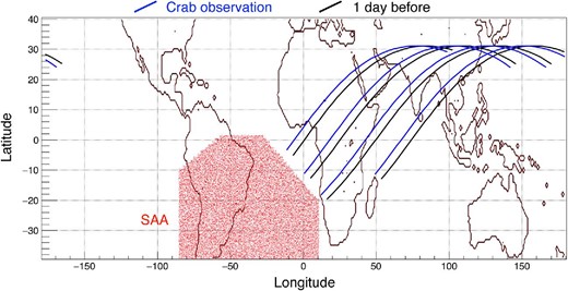
Satellite position during observations. The black line shows the satellite position during the Crab GTI, and the blue line shows the position during the epoch one day earlier.
Time intervals of pointings performed one day earlier than the Crab GTI.
| TSTART [s]* | TSTART [UTC] | TSTOP [s]* | TSTOP [UTC] | Duration [s] |
|---|---|---|---|---|
| 70288549.000000 | 2016/03/24 12:35:48 | 70288579.000000 | 2016/03/24 12:36:18 | 30 |
| 70288627.000000 | 2016/03/24 12:37:06 | 70290952.000000 | 2016/03/24 13:15:51 | 2325 |
| 70294342.000000 | 2016/03/24 14:12:21 | 70296714.000000 | 2016/03/24 14:51:53 | 2372 |
| 70300333.000000 | 2016/03/24 15:52:12 | 70302475.000000 | 2016/03/24 16:27:54 | 2142 |
| 70306319.000000 | 2016/03/24 17:31:58 | 70308079.234375 | 2016/03/24 18:01:18.234375 | 1760 |
* TSTART and TSTOP are expressed in AHTIME, defined as the time elapsed since 2014/01/01 00:00:00 in seconds.
In order to confirm that the satellite encountered similar background environments during similar orbit conditions, we compare the SGD data between an epoch one day earlier and also two days earlier than the Crab observation GTIs. The single-hit spectra obtained by the CdTe side sensors are shown in figure 2. The CdTe side sensors are located on the four sides around the stack of Si/CdTe sensors inside the Compton camera, and are not exposed to gamma-rays from the field of view. Therefore, the influence of the background environment should be reflected strongly in the single-hit events in the CdTe side detectors. The red and black points show the spectra for the epochs one day and two days earlier than the Crab GTI, respectively. These two spectra have the same spectral shape, including various emission lines from activated materials. The flux levels were the same within 3%. On the other hand, the blue spectrum shows the single-hit events of CdTe side detectors on an orbit where the satellite did not pass the SAA region. Although the background environment varied during one day, it was found that background estimation becomes possible by using the data from one day earlier.
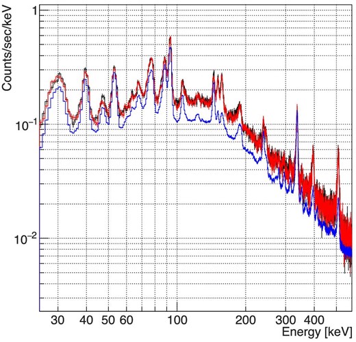
Spectra of CdTe side single-hit events. The red and black points show the spectra for one day and two days earlier than the Crab GTI, respectively. The blue spectrum shows the single-hit events of the CdTe side sensors on an orbit when the satellite did not pass the SAA region.
In order to further verify the background subtraction using the data from one day earlier, the count rates as a function of time during the Crab GTI and one day earlier are compared in figure 3. The red and blue points show the count rates during the Crab GTI and one day earlier. The black points show the count rates of the Crab GTI after subtracting the count rates one day earlier, which corresponds to the count rates of the Crab nebula. Since the black points do not show any visible systematic trend implying additional backgrounds, it implies that this background subtraction is appropriate.
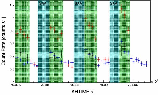
Count rate of the SGD Compton camera as a function of time. The red and blue points show the count rates during the Crab observation and one day earlier. The black points show the count rates of the Crab GTI after subtracting the count rates one day earlier. The regions filled in green show the Crab GTI. The regions filled in cyan show time intervals excluded from the GTI due to the SAA passages. In the “white” portions of the time intervals, the Crab nebula was not able to be observed because of Earth occultation.
3 Data analysis
3.1 Data processing with Hitomi tools
The data processing and event reconstruction were performed by the standard Hitomi pipeline using the Hitomi ftools (Angelini et al. 2018).1 In the pipeline process for SGD, the ftools used for the SGD were hxisgdsff, which converts the raw event data into the predefined data format, hxisgdpha, which calibrates the event energy, and sgdevtid, which reconstructs each event. These tools were included in HEASoft after version 6.19. The version of the calibration files used in this processing was 20140101v003.
3.2 Processing of Crab observation data
Figure 4 shows the relation between OFFAXIS and energy spectrum for the “Compton-reconstructed” events where sgdevtid found the position of the first Compton scattering with physical cos θK in the Si sensors. The histogram in the left-hand panel is made from the events during the Crab GTI, and that in the right-hand panel is made from the events collected one day earlier than the Crab GTI. An excess at around OFFAXIS ∼0° can be seen in the histogram of the Crab GTI corresponding to the gamma-rays from the Crab nebula.
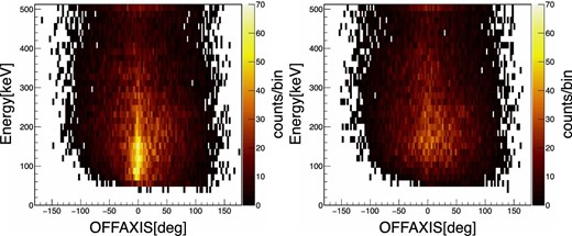
Two-dimensional histograms of Compton-reconstructed events. The relation between OFFAXIS and energy is shown. The left-hand panel is the histogram made from the events during the Crab GTI; the right-hand panel is prepared from the events collected one day earlier than the Crab GTI.
In order to obtain a good signal-to-noise ratio, selections of 60 keV < Energy < 160 keV, −30° < OFFAXIS < +30°, 50° < θgeometry < 150° were applied. The histograms of Energy, OFFAXIS, and θgeometry are shown in figure 5. The selections of Energy, OFFAXIS, and θgeometry were not applied in the histograms of Energy, OFFAXIS, and θgeometry, respectively. The red histograms are made from the events during the Crab GTI, and the events collected during the period one day earlier than the Crab GTI are shown in black as a reference.
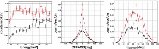
Histograms of Energy, OFFAXIS, θgeometry. The selection criteria were 60 keV < Energy < 160 keV, −30° < OFFAXIS < +30°, and 50° < θgeometry < 150°. The red histograms are made from the events during the Crab GTI, and the black ones are from the events during the epoch one day earlier than the Crab GTI.
We measured the gamma-ray polarization by investigating the azimuth angle distribution in the Compton camera, since gamma-rays tend to be scattered perpendicular to the direction of the polarization vector of the incident gamma-ray in Compton scatterings. Figure 6 shows the azimuth angle distribution of Compton events obtained with the SGD Compton cameras. The red and the black points show the distribution during the Crab GTI and that from one day earlier than the Crab GTI, respectively. The azimuthal angle Φ is defined as the angle from the satellite +X-axis to the satellite +Y-axis. The average count rate during the Crab GTI was 0.808 count s−1.
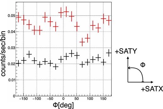
Azimuth angle distributions obtained with the SGD Compton cameras. The red and black points show the distribution during the Crab GTI and that from an epoch one day earlier than the Crab GTI, respectively. The definition of Φ is also shown. SATX and SATY mean the satellite +X-axis and the satellite +Y-axis, respectively.
3.3 Background estimation for polarization analysis
Before the Crab observations, Hitomi also observed RXJ 1856.5−3754, which is fairly faint in the energy band of the SGD (Hitomi Soft X-ray Imager results were reported in Nakajima et al. 2018). The GTIs of RXJ 1856.5−3754 and the exposure times are listed in tables 4 and 5, respectively. The total exposure time of the RXJ 1856.5−3754 observation was about 85.6 ks, and the number of Compton-reconstructed events about 24400. More than ten times the number of events are available by using this observation than the observation of the Crab nebula. In order to obtain the azimuth angle distribution of the background events with better statistics, the SGD data during the RXJ 1856.5−3754 GTI were investigated.
Good time intervals of the RXJ 1856.5−3754 observation.
| TSTART [s]* | TSTART [UTC] | TSTOP [s]* | TSTOP [UTC] | Duration [s] |
|---|---|---|---|---|
| 70207640 | 2016/03/23 14:07:19 | 70212120 | 2016/03/23 15:21:59 | 4480 |
| 70213720 | 2016/03/23 15:48:39 | 70218300 | 2016/03/23 17:04:59 | 4580 |
| 70219740 | 2016/03/23 17:28:59 | 70221820 | 2016/03/23 18:03:39 | 2080 |
| 70221860 | 2016/03/23 18:04:19 | 70224420 | 2016/03/23 18:46:59 | 2560 |
| 70225700 | 2016/03/23 19:08:19 | 70230580 | 2016/03/23 20:29:39 | 4880 |
| 70231600 | 2016/03/23 20:46:39 | 70236720 | 2016/03/23 22:11:59 | 5120 |
| 70237100 | 2016/03/23 22:18:19 | 70274520 | 2016/03/24 08:41:59 | 37420 |
| 70275720 | 2016/03/24 09:01:59 | 70280400 | 2016/03/24 10:19:59 | 4680 |
| 70287960 | 2016/03/24 12:25:59 | 70292460 | 2016/03/24 13:40:59 | 4500 |
| 70294120 | 2016/03/24 14:08:39 | 70298640 | 2016/03/24 15:23:59 | 4520 |
| 70300140 | 2016/03/24 15:48:59 | 70304760 | 2016/03/24 17:05:59 | 4620 |
| 70306140 | 2016/03/24 17:28:59 | 70310880 | 2016/03/24 18:47:59 | 4740 |
| 70312120 | 2016/03/24 19:08:39 | 70317050 | 2016/03/24 20:30:49 | 4930 |
| 70317950 | 2016/03/24 20:45:49 | 70355100 | 2016/03/25 07:04:59 | 37150 |
* The unit for TSTART and TSTOP is AHTIME.
Exposures of the RXJ 1856.5−3754 observation.
| Live time | |
|---|---|
| SGD1 CC1 | 84358.5 |
| SGD1 CC2 | 84432.5 |
| SGD1 CC3 | 84559.5 |
| SGD2 CC1 | 89159.2 |
| Live time | |
|---|---|
| SGD1 CC1 | 84358.5 |
| SGD1 CC2 | 84432.5 |
| SGD1 CC3 | 84559.5 |
| SGD2 CC1 | 89159.2 |
Exposures of the RXJ 1856.5−3754 observation.
| Live time | |
|---|---|
| SGD1 CC1 | 84358.5 |
| SGD1 CC2 | 84432.5 |
| SGD1 CC3 | 84559.5 |
| SGD2 CC1 | 89159.2 |
| Live time | |
|---|---|
| SGD1 CC1 | 84358.5 |
| SGD1 CC2 | 84432.5 |
| SGD1 CC3 | 84559.5 |
| SGD2 CC1 | 89159.2 |
Comparisons of the incident energy, OFFAXIS, θgeometry, and the azimuth angle Φ between the RXJ 1856.5−3754 GTI and one day earlier than the Crab GTI are shown in figure 7. Since orbits with no SAA passage are included in the RXJ 1856.5−3754 observation, the flux level was lower than that obtained one day earlier than the Crab GTI. The count rate of the events during the RXJ 1856.5−3754 GTI was 0.285 count s−1, and that one day earlier than the Crab GTI was 0.404 count s−1. Therefore, the scale of the histograms for the RXJ 1856.5−3754 GTI are normalized to match those for one day earlier than the Crab GTI. The distributions of OFFAXIS, θgeometry, and the azimuth angle Φ are similar. Since the incident energy spectrum of the RXJ 1856.5−3754 GTI looks slightly different from that observed one day earlier than the Crab GTI, we further investigated the effect on the Φ distribution. We divided the data into five energy bands, 60–80 keV, 80–100 keV, 100–120 keV, 120–140 keV, and 140–160 keV, and the number of events in each energy band was normalized to match those for one day earlier than the Crab GTI. The resulting Φ distribution for the RXJ 1856.5−3754 GTI is shown as the magenta points in the lower-right panel of figure 7. We do not observe any significant trend from the original distribution for the RXJ 1856.5−3754 GTI, which implies that the difference in the energy spectrum does not have a significant effect on the Φ distribution. From the above investigations, we conclude that the Compton-reconstructed events during the RXJ 1856.5−3754 GTI can be utilized for the background estimation of the polarization analysis.
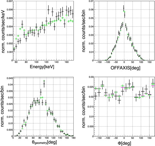
Comparisons between the RXJ 1856.5−3754 observation and those obtained one day earlier than the Crab GTI. The green and black points show the RXJ 1856.5−3754 observation data and the data from one day earlier than the Crab GTI, respectively. The black data points are identical to the black points in figures 5 and 6. The normalizations of the histograms for the RXJ 1856.5−3754 observation are scaled to match the count rate of the one day earlier Crab GTI.
3.4 Monte Carlo simulation
Monte Carlo simulations of SGD are essential to derive the physical parameters, including the gamma-ray polarization, from the observation data. For the Monte Carlo simulations, we used ComptonSoft3 in combination with a mass model of the SGD and databases describing detector parameters that affect the detector response to polarized gamma rays. ComptonSoft is a general-purpose simulation and analysis software suite for semiconductor radiation detectors including Compton cameras (Odaka et al. 2010), and depends on the Geant4 toolkit library (Agostinelli et al. 2003; Allison et al. 2006, 2016) for the Monte Carlo simulation of gamma-rays and their associated particles. We chose Geant4 version 10.03.p03 and G4EmLivermorePolarizedPhysics as the physics model of electromagnetic processes. The mass model describes the entire structure of one SGD unit, including the surrounding BGO shields. The databases of the detector parameters contain configuration of readout electrodes, charge collection efficiencies, energy resolutions, trigger properties, and data readout thresholds in order to obtain accurate detector responses of the semiconductor detectors and scintillators composing the SGD unit.
The format of the simulation output file is same as the SGD observation data. The simulation data can be processed with sgdevtid and, as a result, it is guaranteed that the same event reconstructions are performed for both observation data and simulation data.
For the Compton camera part, the accuracy of the simulation response to the gamma-ray photons and the gamma-ray polarization was confirmed through polarized gamma-ray beam experiments performed at SPring-8 (Katsuta et al. 2016). The better than 3% systematic uncertainty was validated in the polarized gamma-ray beam experiments. On the other hand, the effective area losses due to the distortions and misalignments of the fine collimators (FCs) are not implemented in the SGD simulator (Tajima et al. 2018). We have not obtained measurements of the FC distortions and misalignments with the calibration observations: this is because the satellite operation was terminated before we had the opportunity to make such measurements. In the simulator, ideal-shape FCs with no distortion and no misalignment are implemented. Since the losses due to the distortions and misalignments of the fine collimators do not affect the azimuthal angle distribution of the Compton scattering, the effects on the polarization measurements are negligible.
In the simulation of the Crab nebula emission we assumed a power-law spectrum, N · (E/1 keV)−Γ, with a photon index (Γ) of 2.1. In the first step, unpolarized gamma-ray photons were assumed. Also, the normalization of the simulation model (N) was derived from the Si single-hit events. Figure 8 shows the Si single-hit spectrum obtained with the four Compton cameras. The background spectrum was estimated from the observations taken one day earlier than those for the Crab GTI, and the background-subtracted spectrum is shown in figure 8, together with the simulated spectrum. By scaling the integrated rate of the simulation spectrum in the 20–70 keV range to match the observed rate we obtained N = 8.23, which corresponds to a flux of 1.89 × 10⁻⁸ erg s−1 cm−2 in the 2–10 keV energy range.

Single-hit spectra in the Si detectors of the Crab observation obtained with the four Compton cameras. The background-subtracted observation spectrum is shown in black, and the simulation spectrum is shown in cyan. In the simulation, a power-law spectrum, N · (E/1 keV)−Γ was assumed, with a photon index (Γ) of 2.1 and N = 8.23.
We compared the Compton-reconstructed events between the observation and the simulation. In figure 9, the distributions of OFFAXIS for the observation and the simulation are shown. The distribution of OFFAXIS for the simulation is slightly narrower than that for the observation. If the same selection of −30° < OFFAXIS <+30° is applied for both events, the observation count rate becomes 8.6% smaller than the simulation count rate. We think that one cause of this discrepancy is in the modeling of the Doppler broadening profile of Compton scattering for electrons in silicon crystals. However, at this time, we have not found a solution to eliminate the discrepancy from first principles. Therefore, by adjusting the OFFAXIS selection value of the simulation, we decided to match the count rate of the simulation to the observed count rate of 0.40 count s−1. The relation between the count rate and the OFFAXIS selection for the simulation events is shown in figure 10. From the relation, we obtained |${22{^{\circ}_{.}}13}$| as the OFFAXIS selection value of the simulation. The effect of adjusting the OFFAXIS selection for the simulation is discussed later in this section.
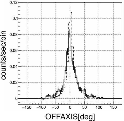
Comparisons of the distributions of OFFAXIS events between the observation and the simulation. The solid line and the dotted line show the observation data and the simulation data, respectively.
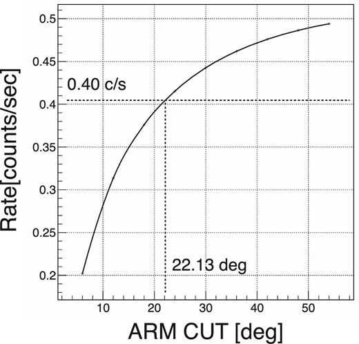
Relation between the count rate and the OFFAXIS selection for the simulation events. The count rate of 0.40 count s−1 derived from the observation data corresponds to the OFFAXIS selection of |${22{^{\circ}_{.}}13}$|.
The observational data, the background data, and the simulation data are plotted in figure 11. The simulation data with the selection of −|${22{^{\circ}_{.}}13}$| < OFFAXIS < +|${22{^{\circ}_{.}}13}$| is shown in black, and the background data derived from the entire RXJ 1856.5−3754 observation is shown in green. The sum of the simulation data and the background data is plotted in blue, and is comparable with the observation data shown in red. The θgeometry distribution is reproduced well by the Monte Carlo simulation, while the energy spectrum shows a small discrepancy due to the background data, as shown in subsection 3.3.
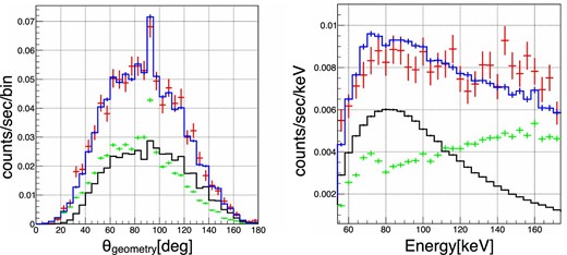
Distribution of θgeometry (left) and the energy spectrum (right). The observational data are plotted in red. The simulation data with the selection of −|${22{^{\circ}_{.}}13}$| < OFFAXIS < +|${22{^{\circ}_{.}}13}$| are shown in black, and, the background data derived from the RXJ 1856.5−3754 observation are shown in green. The sum of the simulation data and the background data is plotted in blue. The red data points are identical to the red ones in figure 5, and the green data points are identical to the green ones in figure 7.
The azimuth angle distributions of the simulated data are shown in figure 12. The left-hand panel shows the azimuth angle distributions of the simulated data with the OFFAXIS selection of −|${22{^{\circ}_{.}}13}$| < OFFAXIS < +|${22{^{\circ}_{.}}13}$| and −30° < OFFAXIS < +30°. The normalization for the −30° < OFFAXIS < +30° selection is scaled. There is little difference in the azimuth angle distribution between these two selections. The right-hand panel of figure 12 shows how the azimuth angle distribution depends on the OFFAXIS selection. It is found that the azimuth angle distribution changes by less than 1% when the angle selection range is changed from 15° to 45°.
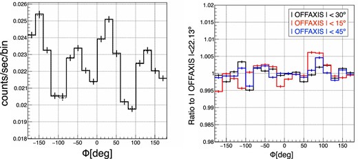
Azimuth angle distributions of simulation data. Left: The azimuth angle distributions of the simulation data with the OFFAXIS selection of −|${22{^{\circ}_{.}}13}$| < OFFAXIS < +|${22{^{\circ}_{.}}13}$| and −30° < OFFAXIS < +30° are shown in the solid line and the dotted line, respectively. The normalization for the −30° < OFFAXIS < +30° selection is scaled. Right: The dependence of the azimuth angle distribution on the selected OFFAXIS value. This is shown as the ratio to the OFFAXIS selection of three values to that limited to −|${22{^{\circ}_{.}}13}$| < OFFAXIS < +|${22{^{\circ}_{.}}13}$|. The black, red, and blue points show the results for OFFAXIS selections of −30° < OFFAXIS < +30°, −15° < OFFAXIS < +15°, and −45° < OFFAXIS < +45°, respectively.
4 Polarization analysis
4.1 Parameter search for the polarization measurement
We obtained the azimuth angle distributions for the Crab observation, the background, and the unpolarized gamma-ray simulation, respectively. In order to derive the polarization parameters of the Crab nebula from these data, we adopted a binned likelihood fit. Although the bin width of the histograms for the azimuth angle distributions was 20° for the figures in the previous subsections, 1° per bin histograms were prepared for the binned likelihood fit. The histograms are shown in figure 13. For the simulation data, the OFFAXIS selection of −|${22{^{\circ}_{.}}13}$| < OFFAXIS < +|${22{^{\circ}_{.}}13}$| was adopted.
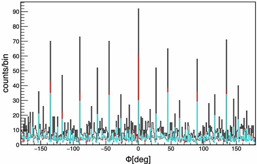
Distributions of the azimuthal angle. The black, red, and cyan lines show the Crab GTI data, the background data derived from the RXJ 1856.5−3754 observation, and simulation data for unpolarized gamma-rays, respectively. Each exposure time is matched with the exposure time of the observation during the Crab GTI. The bin width is 1°.
The errors in the estimated value were evaluated from the confidence level. In the large data sample limit, the difference of the log likelihood |$\mathcal {L}$| from the minimum |$\mathcal {L}_0$|, |$\Delta \mathcal {L}=\mathcal {L}-\mathcal {L}_0$|, follows χ2. Since we have two free parameters, |$\Delta \mathcal {L}$|s of 2.30, 5.99, 9.21 correspond to the coverage probabilities of 68.3%, 95.0%, and 99.0%, respectively.
4.2 Polarization results and validation
The dependence of |$\mathcal {L}$| on Q and ϕ0 is shown in figure 14. The best-fit parameters of Q and ϕ0 are Q = 0.1441 and ϕ0 = |${67{^{\circ}_{.}}02}$|. The contours in figure 14 show |$\Delta \mathcal {L} = 2.30$|, 5.99, 9.21. The errors corresponding to the |$\Delta \mathcal {L} = 2.30$| level (1 σ) are −0.0688, +0.0688 for Q and −|${13{^{\circ}_{.}}15}$|, +|${13{^{\circ}_{.}}02}$| for ϕ0. We also derived the log likelihood at Q = 0 (|$\mathcal {L}_{Q=0}$|), and then the difference between |$\mathcal {L}_{Q=0}$| and |$\mathcal {L}_0$| is found to be 10.03.
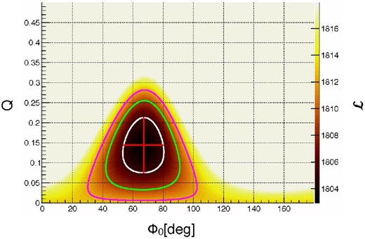
Results of the maximum log likelihood estimation for the Crab observation data. The best-fit parameters are shown with a red cross. Contours of the |$\Delta \mathcal {L}$|s of 2.30, 5.99, and 9.21 are shown as the white line, the green line, and the magenta line, respectively. In the large-sample limit, they correspond to the coverage probabilities of 68.3%, 95.0%, and 99.0%, respectively. The best-fit parameters are Q = 0.1441 and |$\phi _0 = {67{^{\circ}_{.}}02}$|. The errors corresponding to the |$\Delta \mathcal {L} = 2.30$| level (1 σ) are −0.069, +0.069, and −|${13{^{\circ}_{.}}2}$|, +|${13{^{\circ}_{.}}0}$| for Q and ϕ0, respectively.
The modulation amplitude for the 100% polarized gamma-ray photons (Q100) is slightly dependent on ϕ0 and was estimated to be Q100 = 0.6534 with the Monte Carlo simulation for ϕ0 = 67° and a power-law spectrum with a photon index (Γ) of 2.1. As a result, the polarization fraction (Π) of the Crab nebula was calculated as Π = 0.1441/0.6534 = 22.1%, and the error was calculated as 0.0688/0.6534 = 10.5%.
In order to validate the statistical confidence, we made 1000 simulated Crab observation data sets and derived the parameters with the binned likelihood fits for each data set. Because the exposure time of the Crab observation was about 5 ks, the exposure time of the simulated Crab observation data was also set to be 5 ks. In the Monte Carlo simulations, the polarization fraction Π = 0.22 and the polarization angle ϕ0 = 67° were assumed. The background data was prepared using the azimuth angle distribution of the background data shown in figure 13. By using a random number according to the azimuth angle distribution of the background data, 1000 sets of 5 ks background data were obtained. The 1000 sets of simulated Crab observation data were prepared by summing each Monte Carlo data and background data.
The distribution of the best combinations of Q and Φ0 from the fits for the 1000 sets of Crab simulation data are shown as the red points of figure 15. The numbers of data sets inside the contours of |$\Delta \mathcal {L}$|s of 2.30, 5.99, and 9.21 are 668, 945, and 984, respectively. These numbers match the coverage probabilities in the case of two parameters.
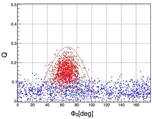
Results of likelihood estimations for 1000 sets of simulation data. The red points show the best-fit parameters for the Crab simulation data with the polarization parameters (Π = 0.22 and ϕ0 = 67°) derived from the observation data, and the blue points show the best-fit parameters for the unpolarized simulation data. The contours are the same as in figure 14.
In order to validate the confidence level for the detection of polarized gamma-rays, we also prepared 1000 sets of unpolarized simulation data. The results of the binned likelihood fits for the data sets are shown in the blue points of figure 15. The distribution of the difference between the minimum of the log likelihood (|$\mathcal {L}_0$|) and the log likelihood of Q = 0 (|$\mathcal {L}_{Q=0}$|) is shown in figure 16. It is confirmed that the value of the difference corresponds to the coverage probabilities in the case of two parameters. Therefore, the |$\Delta \mathcal {L}$| against the case of Q = 0 of 10.03 derived from the Crab observation corresponds to a confidence level of 99.3%.
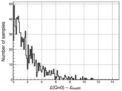
Histogram of the difference between the minimum of the log likelihood |$\mathcal {L}$| and the log likelihood of Q = 0 for the 1000 sets of unpolarized simulation data. The numbers of data sets within the differences of 2.30, 5.99, and 9.21 are 668, 955, and 993, respectively. The difference between the minimum of the log likelihood |$\mathcal {L}$| and the log likelihood of Q = 0 also corresponds to the coverage probability for two parameters.
Figure 17 shows the phi distribution of the gamma rays from the Crab nebula with the parameters determined in this analysis. Figure 18 shows the relation between the satellite coordinate and the sky coordinate. The roll angle during the Crab observation was |${267{^{\circ}_{.}}72}$|; ϕ0 = |${67{^{\circ}_{.}}02}$| then corresponds to a polarization angle of |${110{^{\circ}_{.}}70}$|.
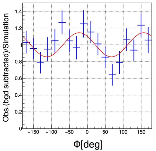
Modulation curve of the Crab nebula observed with SGD. The data points show the ratio of the background-subtracted observation data to the unpolarized simulation data. The error bar size indicates their statistical errors. The red curve shows the sine curve function substituting the estimated parameters by the log-likelihood fitting.
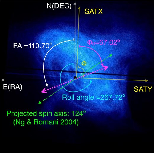
Polarization angle of the gamma-rays from the Crab nebula determined by SGD. The direction of the polarization angle is drawn on the X-ray image of Crab with Chandra.
5 Discussion
5.1 Comparison with other measurements
The detection of polarization, and the measurement of its angle, indicates the direction of an electric field vector of radiation. In our analysis, the polarization angle is derived to be PA|$= {110{^{\circ}_{.}}7}^{+{13{^{\circ}_{.}}2}}_{- {13{^{\circ}_{.}}0}}$|. The energy range of gamma-rays contributing most significantly to this measurement is ∼60–160 keV. All pulse phases of the Crab nebula emission were integrated. The spin axis of the Crab pulsar is estimated to be |${124{^{\circ}_{.}}0}\, \pm \, {0{^{\circ}_{.}}1}$| from X-ray imaging (Ng & Romani 2004). Therefore, the direction of the electric vector of radiation as measured by the SGD is about one standard deviation with the spin axis.
The Crab polarization observation results from other instruments are listed in table 6. These instruments can be divided into three types based on the material of the scatterer. PoGO+ and the SGD employ carbon and silicon for a scatterer, respectively, while the remaining instruments employ CZT or germanium. The cross section of the Compton scattering exceeds that of the photo absorption at around 20 keV for carbon, around 60 keV for silicon, and above 150 keV for germanium and CZT, which constrains the minimum energy range for each instrument. Since the flux decreases with E−2, the effective maximum energy for polarization measurements will be less than four times the minimum energy. Therefore, PoGO+, SGD, and the other instruments have more or less non-overlapping energy ranges and are complementary. The PoGO+ team has reported the polarization angle PA|$= {131{^{\circ}_{.}}3}\, \pm {6{^{\circ}_{.}}8}$| and the polarization fraction PF =20.9% ± 5.0% for the pulse-integrated period, and PA =137° ± 15° and PF|$= 17.4\%^{+8.6\%}_{-9.3\%}$| for the off-pulse period (Chauvin et al. 2017). Our results are consistent with the PoGO+ results. On the other hand, for the higher energy range, INTEGRAL IBIS, SPI, and AstroSat CZTI have performed polarization observations of the Crab nebula in recent years, and reported slightly higher polarization fractions than our results. Furthermore, AstroSat CZTI reported varying polarization fractions during the off-peak period (Vadawale et al. 2017). However, we have not been able to verify those results because of the extremely short observation time, which was less than 1/18th of PoGO+, and less than 1/100th of the higher-energy instrument. Despite such a short observation time, the errors of our measurements are within a factor of two of the other instruments. This result demonstrates the effectiveness of the SGD design, such as the high modulation factor of the azimuthal angle dependence, highly efficient instrument design, and low backgrounds. Extrapolating from this result, we expect that a 20 ks SGD observation can achieve statistical errors equivalent to PoGO+ and AstroSAT CZTI, and an 80 ks SGD observation could perform phase-resolved polarization measurements with similar errors.
Crab polarization observation results.
| Satellite/instruments | Energy band | Polarization | Polarization | Exposure | Phase | Supplement |
|---|---|---|---|---|---|---|
| angle [°] | fraction [%] | time | ||||
| PoGO+ (Balloon exp.) | 20–160 keV | 131.3 ± 6.8 | 20.9 ± 5.0 | 92 ks | All | Chauvin et al. (2017) |
| Hitomi/SGD | 60–160 keV | |$110.7^{+13.2}_{-13.0}$| | 22.1 ± 10.6 | 5 ks | All | This work |
| AstroSat/CZTI | 100–380 keV | 143.5 ± 2.8 | 32.7 ± 5.8 | 800 ks | All | Vadawale et al. (2017) |
| INTEGRAL/SPI | 130–440 keV | 117 ± 9 | 28 ± 6 | 600 ks | All | Chauvin et al. (2013) |
| INTEGRAL/IBIS | 200–800 keV | 110 ± 11 | |$47^{+19}_{-13}$| | 1200 ks | All | Forot et al. (2008) |
5.2 Implications for the source configuration
We made a simple model of the polarization by assuming that the magnetic field is purely toroidal and the particle distribution function is isotropic (cf. Woltjer 1958). The observed synchrotron radiation should be polarized along the projected symmetry axis (e.g., Rybicki & Lightman 1979). The degree of polarization depends on the spectral index α ≡ −(1 + d ln Nx/d ln EX), where NX is the number of photons per unit photon energy EX. It can be simply calculated by integration over the azimuthal angle ϕ around a circular ring with axis inclined at an angle θ to the line of sight, |$\boldsymbol n$|. In these coordinates, |$\hat{\boldsymbol B}\cdot \hat{\boldsymbol n}=\sin \theta \sin \phi$|, and the angle χ between the local and and the mean polarization direction satisfies cos 2χ = (cos 2ϕ − cos 2θsin 2ϕ)/(1 − sin 2θsin 2ϕ). The mean degree of polarization is then given by
For the measured parameters, α = 1.1, θ = 60°, this evaluates to Π = 0.37. The measured mean polarization is comfortably below this value, suggesting that the magnetic field is moderately disordered relative to our simple model and the particle distribution function may be anisotropic. Magnetohydrodynamic and particle-in-cell simulations can be used to investigate this further.
6 Conclusions
The Soft Gamma-ray Detector (SGD) on board the Hitomi satellite observed the Crab nebula during the initial test observation period of Hitomi. Even though this observation was not intended for scientific analysis, the gamma-ray radiation from the Crab nebula was detected by combining careful data analysis, background estimation, and SGD Monte Carlo simulations. Moreover, polarization measurements were performed for the data obtained with SGD Compton cameras, and polarization of soft gamma-ray emission was successfully detected. The obtained polarization fraction of the phase-integrated Crab emission (sum of pulsar and nebula emissions) was 22.1% ± 10.6%, and the polarization angle was |${110{^{\circ}_{.}}7}$| +|${13{^{\circ}_{.}}2}$|/−|${13{^{\circ}_{.}}0}$| (the errors correspond to a 1 σ deviation) despite an extremely short observation time of 5 ks. The confidence level of the polarization detection was 99.3%. This is well described as the soft gamma-ray emission arising predominantly from energetic particles radiating via the synchrotron process in the toroidal magnetic field in the Crab nebula, roughly symmetric around the rotation axis of the Crab pulsar. This result demonstrates that the SGD design is highly optimized for polarization measurements.
Acknowledgments
We thank all the JAXA members who have contributed to the ASTRO-H (Hitomi) project. All US members gratefully acknowledge support through the NASA Science Mission Directorate. The Stanford and SLAC members acknowledge support via DoE contract to SLAC National Accelerator Laboratory DE-AC3-76SF00515 and NASA grant NNX15AM19G. Part of this work was performed under the auspices of the US DoE by LLNL under Contract DE-AC52-07NA27344. Support from the European Space Agency is gratefully acknowledged. The French members acknowledge support from CNES, the Centre National d’Études Spatiales. SRON is supported by NWO, the Netherlands Organization for Scientific Research. The Swiss team acknowledges the support of the Swiss Secretariat for Education, Research and Innovation (SERI). The Canadian Space Agency is acknowledged for the support of the Canadian members. We acknowledge support from JSPS/MEXT KAKENHI grant numbers 15H00773, 15H00785, 15H02090, 15H03639, 15H05438, 15K05107, 15K17610, 15K17657, 16J02333, 16H00949, 16H06342, 16K05295, 16K05296, 16K05300, 16K13787, 16K17672, 16K17673, 17H02864, 17K05393, 17J04197, 21659292, 23340055, 23340071, 23540280, 24105007, 24244014. 24540232, 25105516, 25109004, 25247028, 25287042, 25287059, 25400236, 25800119, 26109506, 26220703, 26400228, 26610047, 26800102, 26800160, JP15H02070, JP15H03641, JP15H03642, JP15H06896, JP16H03983, JP16K05296, JP16K05309, and JP16K17667. The following NASA grants are acknowledged: NNX15AC76G, NNX15AE16G, NNX15AK71G, NNX15AU54G, NNX15AW94G, and NNG15PP48P to Eureka Scientific. This work was partly supported by Leading Initiative for Excellent Young Researchers, MEXT, Japan, and also by the Research Fellowship of JSPS for Young Scientists. H. Akamatsu acknowledges the support of NWO via a Veni grant. C. Done acknowledges STFC funding under grant ST/L00075X/1. A. Fabian and C. Pinto acknowledge ERC Advanced Grant 340442. P. Gandhi acknowledges a JAXA International Top Young Fellowship and UK Science and Technology Funding Council (STFC) grant ST/J003697/2. Y. Ichinohe, K. Nobukawa, and H. Seta are supported by the Research Fellow of JSPS for Young Scientists program. N. Kawai is supported by the Grant-in-Aid for Scientific Research on Innovative Areas “New Developments in Astrophysics Through Multi-Messenger Observations of Gravitational Wave Sources.” S. Kitamoto is partially supported by the MEXT Supported Program for the Strategic Research Foundation at Private Universities, 2014–2018. B. McNamara and S. Safi-Harb acknowledge support from NSERC. T. Dotani, T. Takahashi, T. Tamagawa, M. Tsujimoto, and Y. Uchiyama acknowledge support from the Grant-in-Aid for Scientific Research on Innovative Areas “Nuclear Matter in Neutron Stars Investigated by Experiments and Astronomical Observations.” N. Werner is supported by the Lendület LP2016-11 grant from the Hungarian Academy of Sciences. D. Wilkins is supported by NASA through Einstein Fellowship grant number PF6-170160, awarded by the Chandra X-ray Center and operated by the Smithsonian Astrophysical Observatory for NASA under contract NAS8-03060.
We acknowledge contributions by many companies, including in particular NEC, Mitsubishi Heavy Industries, Sumitomo Heavy Industries, Japan Aviation Electronics Industry, Hamamatsu Photonics, Acrorad, Ideas, SUPER RESIN, and OKEN. We acknowledge strong support from the following engineers. JAXA/ISAS: Chris Baluta, Nobutaka Bando, Atsushi Harayama, Kazuyuki Hirose, Kosei Ishimura, Naoko Iwata, Taro Kawano, Shigeo Kawasaki, Kenji Minesugi, Chikara Natsukari, Hiroyuki Ogawa, Mina Ogawa, Masayuki Ohta, Tsuyoshi Okazaki, Shin-ichiro Sakai, Yasuko Shibano, Maki Shida, Takanobu Shimada, Atsushi Wada, and Takahiro Yamada; JAXA/TKSC: Atsushi Okamoto, Yoichi Sato, Keisuke Shinozaki, and Hiroyuki Sugita; Chubu University: Yoshiharu Namba; Ehime University: Keiji Ogi; Kochi University of Technology: Tatsuro Kosaka; Miyazaki University: Yusuke Nishioka; Nagoya University: Housei Nagano; NASA/GSFC: Thomas Bialas, Kevin Boyce, Edgar Canavan, Michael DiPirro, Mark Kimball, Candace Masters, Daniel Mcguinness, Joseph Miko, Theodore Muench, James Pontius, Peter Shirron, Cynthia Simmons, Gary Sneiderman, and Tomomi Watanabe; ADNET Systems: Michael Witthoeft, Kristin Rutkowski, Robert S. Hill, and Joseph Eggen; Wyle Information Systems: Andrew Sargent and Michael Dutka; Noqsi Aerospace Ltd: John Doty; Stanford University/KIPAC: Makoto Asai and Kirk Gilmore; ESA (Netherlands): Chris Jewell; SRON: Daniel Haas, Martin Frericks, Philippe Laubert, and Paul Lowes; University of Geneva: Philipp Azzarello; CSA: Alex Koujelev and Franco Moroso. Finally, we greatly appreciate the dedicated work by all students in participating institutions.
Author contributions
S. Watanabe led this study in data analysis and writing drafts. He also contributed to the SGD overall design, fabrication, integration and tests, in-orbit operations, and calibration. Y. Uchida contributed to data analysis and preparing the drafts, in addition to the SGD calibration. H. Odaka worked on the SGD Monte Carlo simulator and contributed to data analysis. G. Madejski contributed to writing drafts and improved the draft. K. Hayashi contributed to the testing and calibration of the SGD and the SGD operations. T. Mizuno contributed to data analysis in addition to the polarized beam experiment. R. Sato and Y. Yatsu worked on the SGD BGO shield design, fabrication, and testing, and also contributed to Hitomi’s operations.
Footnotes
The corresponding authors are Shin Watanabe, Yuusuke Uchida, Hirokazu Odaka, Greg Madejski, Katsuhiro Hayashi, Tsunefumi Mizuno, Rie Sato, and Yoichi Yatsu.
The details of the columns recorded are shown at 〈https://heasarc.gsfc.nasa.gov/ftools/caldb/help/sgdevtid.html〉.
References
