Blue-wing enhancement of the chromospheric Mg ii h and k lines in a solar flare

Abstract

1 Introduction

A solar flare is one of the most energetic phenomena observed in the solar atmosphere, releasing a huge amount of energy of up to 10³² erg on a typical timescale of from minutes to tens of minutes. The magnetic energy in the solar atmosphere is released through magnetic reconnection and converted to various kinds of energy: kinetic energy of mass ejection, thermal energy of hot plasma, and non-thermal energy of accelerated particles (Shibata & Magara 2011). On the basis of observations and theories, the standard flare reconnection model has been developed (Carmichael 1964; Sturrock 1966; Hirayama 1974; Kopp & Pneuman 1976). From the viewpoint of energy transport, it is unclear not only where and how the energy is released, transported, and converted to thermal or kinetic energy, but also how the lower atmosphere responds to the energy input. In chromospheric lines, such as Hα and Ca ii H and K, a pair of long, curved bright areas (flare ribbons) and strongly bright patches in flare ribbons (flare kernels) have been observed during flares (Svestka 1976). Such chromospheric flares are thought to be excited by energy transferred from the corona into the chromosphere.

A number of authors have proposed mechanisms of energy transport from the flare site in the corona to the chromosphere: e.g., electron beams (Brown 1973), thermal conduction (Hirayama 1974), soft X-ray (SXR) irradiation (Henoux & Nakagawa 1978), ion beams (Lin et al. 2003), and Alfvén waves (Fletcher & Hudson 2008). A beam of accelerated (non-thermal) electrons is a key mechanism that has been widely discussed, since a strong enhancement of chromospheric (and occasionally photospheric) emission is temporally and spatially correlated with hard X-ray (HXR) emission and microwave radiation (e.g., Asai et al. 2012) that are generated by the non-thermal bremsstrahlung (Brown 1971) and gyrosynchrotron emission (Takakura & Kai 1966), respectively.

In relation to such chromospheric heating, a hot (8–25 MK) and dense upflow (up to 400 km s⁻¹) along the flare loops has been detected in the wavelength range of SXR and extreme ultraviolet (EUV) during flares (Doschek et al. 1980; Antonucci et al. 1982; Strong et al. 1984; Milligan 2015), which is called chromospheric evaporation. In the chromospheric-evaporation scenario, high-energy (accelerated) particles enter and collide with the chromospheric plasma, which causes a rapid increase of temperature and pressure in the chromosphere (Hirayama 1974; Fisher et al. 1985). The heated plasma expands drastically upward along the magnetic field lines at almost its sound speed. As a result, the plasma is observed as coronal hot loops in the SXR and EUV. At the same time, the chromospheric plasma is strongly compressed and the downward-propagating shock waves are excited in the chromosphere, because of the low chromospheric sound speed. In this compressed region, radiative cooling becomes so effective that the temperature does not increase very much. Consequently, the density increases more to maintain the pressure balance, which leads to further effective radiation. Therefore, the chromospheric condensation accompanying the strong compression and the downflow takes place.

Indeed, redshifts and enhancements in the red wing (red asymmetry) have been observed in the chromospheric lines during the impulsive phase of flares (e.g., Švestka et al. 1962; Ichimoto & Kurokawa 1984; Shoji & Kurokawa 1995; Ding et al. 1995), which can be explained by the condensation downflow in the chromosphere. Ichimoto and Kurokawa (1984) measured redshifts and downward Doppler velocities in the Hα line during flares quantitatively, and established that the downflow (∼50 km s⁻¹) can be explained by the momentum balance with the chromospheric-evaporation upflow. This was confirmed by Shoji and Kurokawa (1995), who investigated other lines, such as Ca ii K and He D₃, as well as the Hα line, and showed that the velocity derived from the Hα spectra was consistent with that from the He D₃ line (50–100 km s⁻¹).

On the other hand, blue asymmetry in the chromospheric lines has also been reported (Švestka et al. 1962; Canfield et al. 1990; Heinzel et al. 1994; Kerr et al. 2015). Švestka, Kopecký, and Blaha (1962) studied the line asymmetry in 244 spectra of 92 individual flares observed in the Hα, Ca ii H and K, and He i lines. They concluded that 80% of the flares show red asymmetry and 23% of the flares contain regions with the blue asymmetry. Furthermore, they showed that the blue asymmetry predominantly occurs in the early phase of the flares. In Heinzel et al. (1994), the Balmer and Ca ii H lines showed the blue asymmetry at the same time during the onset phase of a flare. Some researchers have attempted to explain the origin of the blue asymmetry (Canfield et al. 1990; Heinzel et al. 1994; Ding & Fang 1997; Kuridze et al. 2015, 2016), but we have not obtained any consensus.

The chromosphere in solar flares has been spectroscopically observed mostly from the ground so far. The frequently used lines have been the Balmer lines (mainly the Hα) and the Ca ii H, K, and 8542 Å lines in visible and near infrared. In addition to these lines, there are several lines in ultraviolet having strong emissions from the chromosphere that are not available in the ground observation. The Mg ii lines are the representative ones. Now we can use the Mg ii h and k lines detected by the Interface Region Imaging Spectrograph (IRIS: De Pontieu et al. 2014), which was launched in 2013. Furthermore, other chromospheric and transitional region lines, such as the C ii and Si iv lines, are also available on IRIS data. With these ultraviolet lines, numerous studies of solar flares have been conducted. Kerr et al. (2015) and Liu et al. (2015) studied the response of the Mg ii lines to solar flares and presented the spatial, temporal behavior of the physical quantities. Kerr et al. (2015) showed very intense, spatially localized energy inputs at the outer edge of the ribbon, resulting in redshifts equivalent to velocities of 15–26 km s⁻¹, line broadenings, and line asymmetry in the most intense sources. Graham and Cauzzi (2015) presented the dynamic evolution of chromospheric evaporation and condensation in a flare ribbon. Successive brightenings in the impulsive phase displayed the same initial coronal upflows of up to 300 km s⁻¹ and chromospheric downflows up to 40 km s⁻¹. Also see Li et al. (2015, 2017) and Brosius and Inglis (2017), which investigated the chromospheric evaporation and condensation using ultraviolet lines by IRIS. Recently, a narrow dark moving feature has been observed at the front of flare footpoints in He i 10830 Å (Xu et al. 2016). Xu et al. (2016) suggest that theoretically the dark feature in He i 10830 Å can be produced under special circumstances by non-thermal electron collisions or photoionization, followed by recombination. This might be related to the blue asymmetry observed in the chromospheric lines.

In this paper, we report on chromospheric dynamics related to a C5.4 flare on 2014 November 11, simultaneously observed with IRIS and the Domeless Solar Telescope (DST: Nakai & Hattori 1985) at Hida Observatory of Kyoto University. We show the temporal, spatial evolution of six chromospheric and transitional region lines in relation to a moving flare kernel that was observed during the impulsive phase of the flare. In section 2, we describe the data set and data reduction. Further, observational description of the flare kernel and our method for analyzing the data are shown in section 3. Section 4 gives the results. Finally, we discuss the interpretation of observational results and present a summary in section 5.

2 The data set and data reduction

We carried out coordinated observations (HOP 275) of NOAA AR 12205, located near the disk center (N13°, W17°) from 2014 November 10 to 11 with IRIS and DST. The active region produced a C5.4 flare that started at |${23^{\rm h}55^{\rm m}}$| UT on November 10, peaked at |${0^{\rm h}01^{\rm m}}$| UT, and ended at |${0^{\rm h}08^{\rm m}}$| UT on November 11 (figure 1).

Fig. 1.

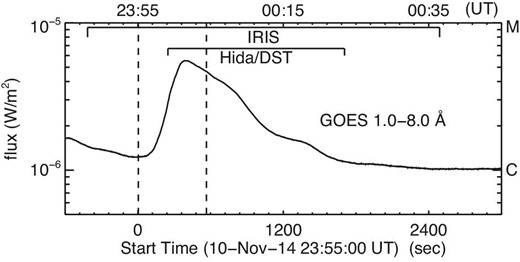
GOES SXR (1.0–8.0 Å) light curve of a C5.4 flare, which started at |${23^{\rm h}55^{\rm m}}$|⁠, peaked at |${00^{\rm h}01^{\rm m}}$|⁠, and ended at |${00^{\rm h}08^{\rm m}}$| (UT) on 2014 November 10 and 11. The upper and lower horizontal axes are the time “hh:mm” (UT) and the elapsed time (s) from the start time of the flare, respectively. Two dashed lines indicate both sides of the time range in figure 2. The observation times of IRIS and Hida DST are also shown.

Open in new tabDownload slide

IRIS observed the flare at the fixed slit location (sit-and-stare mode) from 23:48:05 UT on November 10 to 00:36:30 UT on November 11 (observation time is shown in figure 1). The field of view (FOV) with the slit-jaw imager (SJI) was 120″ × 162″ by a sampling of 0|${^{\prime\prime}_{.}}$|166 pixel⁻¹. The spatial sampling along the IRIS slit by the spectrograph was also 0|${^{\prime\prime}_{.}}$|166 pixel⁻¹. The temporal cadence was 9.5 s for the spectral data and 29 s for the SJI filtergrams. In this study, we used the Mg ii h 2803 Å, Mg ii k 2796 Å, C ii 1335 Å, and Si iv 1403 Å lines, which have formation temperatures of Log T [K] = 4.0, 4.0, 4.3, and 4.8, respectively (De Pontieu et al. 2014). We used mainly the Mg ii h line rather than the Mg ii k line, because another line locates in the blue wing of the Mg ii k line, which causes difficulties concerning correct measurements of the characteristic parameters of the line, as described later. The Mg ii k line behaves similarly and has a relatively higher intensity than the Mg ii h line. We note that the signal from the Fe xxi line, which can be used for the indication of the coronal evaporation upflow, was too weak to be detected.

DST observed the flare from 23:59:08 UT on November 10 to 00:23:25 UT on November 11 (as shown in figure 1). Raster-scanned maps by the slit, which moved from west to east on the solar surface, were obtained with the horizontal spectrograph on DST with a repeat cadence of 10 s. We used the spectral data of the Ca ii K 3934 Å, Ca ii 8542 Å, and Hα 6563 Å lines, which all form at around the chromospheric temperature (∼10⁴ K). The data were taken by three identical cameras, Prosilica GE1650, and the timing to obtain the data was synchronized in all of the cameras. The spatial samplings in the direction perpendicular to the slit were 0|${^{\prime\prime}_{.}}$|64 pixel⁻¹ and those along the slit for the Ca ii K, Ca ii 8542 Å, and Hα lines were 0|${^{\prime\prime}_{.}}$|27 pixel⁻¹, 0|${^{\prime\prime}_{.}}$|28 pixel⁻¹, and 0|${^{\prime\prime}_{.}}$|36 pixel⁻¹, respectively. We note that the actual spatial resolution was about 2″ due to the seeing effect. The spectral sampling and the velocity that corresponds to the spectral sampling were 15 mÅ pixel⁻¹ and 1.1 km s⁻¹ for the Ca ii K line, 15 mÅ pixel⁻¹ and 0.5 km s⁻¹ for the Ca ii 8542 Å line, and 22 mÅ pixel⁻¹ and 1.0 km s⁻¹ for the Hα line. We used spectral data smoothed over ±5, ±15, and ±10 data points along the wavelength for the Ca ii K, Ca ii 8542 Å, and Hα lines, respectively, because the physical parameters could not be derived due to their low signal-to-noise ratio. This smoothing does not affect the measurements of velocities described in the section 3. Smoothing leads an artificial broadening of profiles, but the absolute values of line widths are not important in this study.

Time profiles of high-energy emissions are obtained with the Nobeyama Radioheliograph (NoRH: Nakajima et al. 1994) and the Fermi/Gamma-ray Burst Monitor (GBM: Meegan et al. 2009). The NoRH data were created by the SSW function “norh_tb2flux,” with the option “abox =[0, 220, 80, 330]” (in units of arcseconds) covering the flare region. The Fermi/GBM n0 detector was best faced toward the Sun during this flare, and was used in this study.

We also used 94 Å, 304 Å, and 1600 Å images of the Atmospheric Imaging Assembly (AIA: Lemen et al. 2012) and continuum images and line-of-sight magnetograms of the Helioseismic and Magnetic Imager (HMI: Scherrer et al. 2012). Both AIA and HMI are installed in the Solar Dynamics Observatory (SDO: Pesnell et al. 2012).

We conducted co-alignments between the data of the different instruments, using images and maps taken at around 23:59:08 UT. First, we aligned the intensity map at the Hα −8 Å from DST to the continuum image of HMI. Secondly, maps in the Ca ii K −5.5 Å and Ca ii 8542 Å −5.0 Å from DST were aligned to the Hα map. Thirdly, the AIA 1600 Å image and the IRIS Si iv image were used for alignment of all SDO images with the IRIS data. By combining these procedures, we can finally remove offsets between images and maps.

3 The flare kernel and its analysis

In order to investigate the energy input and the dynamics, we looked at a flare kernel that appeared during the impulsive phase of the flare. Here is a description of the flare kernel on which we focus in this paper. We define two variables, t and y_slit, as the elapsed time from the flare onset at 23:55:00 UT and the y position along the IRIS slit in the solar coordinates, respectively. Figure 2 shows the temporal variation of high-energy emissions around the impulsive phase (t = 150–360 s), which indicates the energy input from the corona to the lower atmosphere. The impulsive phase consists of two bursts. The first one was involved in the NoRH 17 GHz and Fermi HXR flux during t = 150–200 s. During the second burst (t = 200–360 s), the time derivative of the GOES SXR and Fermi HXR flux increased. Figure 3 shows images of the flare region at the flare peak time. There were two sets of two conjugate flare ribbons. Each set was at the northern and southern parts of FOV of figure 3. The northern flare ribbons (FR|$_{\rm N}^+$| and FR|$_{\rm N}^-$|⁠) were at two sides of the magnetic polarity inversion line of the delta-type sunspot. The southern flare ribbons (FR|$_{\rm S}^+$| and FR|$_{\rm S}^-$|⁠) were involved in the mixed polarity region to the south of the delta-type sunspot. The flare kernel we focus on was located in FR|$_{\rm S}^-$| [on the IRIS slit (y_slit ∼174″ in figures 3c–3d)]. As shown in figure 4, the intensity of the flare ribbon was weak during the first burst, and became much higher at t ∼200 s. Note that the increase of the NoRH 17 GHz microwave in the first burst (t = 150–200 s in figure 2c) was involved in the northern flare (see figure 3a), which is out of our scope. During the second burst (t = 200–360 s), the flare kernel moved ∼9″ northward along the slit with an apparent speed of 31 km s⁻¹. At t ∼ 360 s, the feature stopped moving in the vicinity of the penumbra and became less bright.

Fig. 2.

Temporal variation of high-energy emissions. (a) GOES SXR flux of the 1.0–8.0 Å channel. (b) Time derivative of the GOES SXR flux. (c) NoRH 17 GHz microwave from the flare region. The preflare flux is subtracted. (d)–(e) Fermi/GBM HXR fluxes in the range of 29–31 keV and 50–100 keV. The horizontal axis is the elapsed time from the start time of the flare. The times of the seven snapshots in figure 4 are indicated by the arrows. The two-arrow line denotes the X (horizontal) range of figure 5 and figure 6. The observation time range of Hida DST is also shown.

Open in new tabDownload slide

Fig. 3.

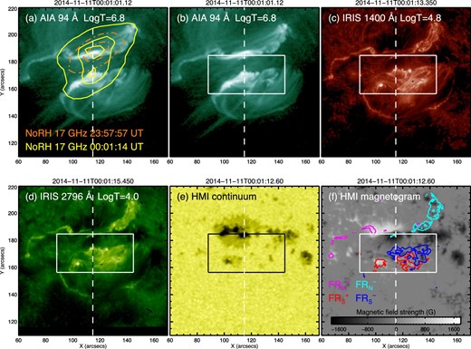
Snapshots of the flare region around the peak time of the flare at |${00^{\rm h}01^{\rm m}}$| UT. (a)–(b) SDO/AIA 94 Å. (c) IRIS SJI 1400 Å. (d) IRIS SJI 2796 Å. (e) SDO/HMI continuum. (f) SDO/HMI line-of-sight magnetogram. Characteristic temperatures are shown in (a)–(d). In panel (a), we overlaid contour images of NoRH 17 GHz: orange dash-dotted contours show 40% and 80% levels of the peak intensity at 23:57:57 UT and yellow solid contours show 40%, 80%, and 94% levels of the peak intensity at 00:01:14 UT. In panel (f), two sets of two conjugate flare ribbons are shown by the overlaid contour image (10% level of the peak intensity of the IRIS SJI 2796 Å): the northern flare ribbons with positive and negative polarity (FR|$_{\rm N}^+$| and FR|$_{\rm N}^-$|⁠) are indicated by magenta and cyan lines, and the southern flare ribbons with positive and negative polarity (FR|$_{\rm S}^+$| and FR|$_{\rm S}^-$|⁠) by red and blue lines, respectively. The vertical-dashed line is the location of the IRIS slit. The white box is the region shown in figure 4. (Color online)

Open in new tabDownload slide

Fig. 4.

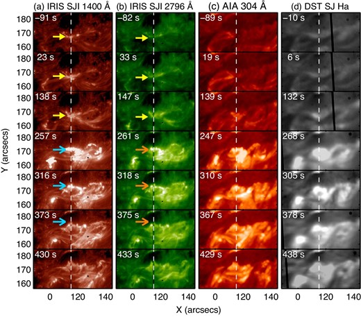
Time series of the flare region in the white box of figure 3. In each panel, the elapsed time from the start time of the flare at |${23^{\rm h}55^{\rm m}}$| UT is shown. The dashed line indicates the IRIS slit location. In (a) and (b), a bright feature staying at the same slit position is indicated by the yellow arrow. The (a) cyan and (b) orange arrows indicate the position of the moving flare kernel. (Color online)

Open in new tabDownload slide

We investigated the temporal, spatial variation of the dynamics around the flare kernel by measuring three quantities of the spectral lines: the peak intensity, line width, and Doppler velocity as well as the first moment velocity (intensity-weighted velocity across the line). The original-line profiles were used to derive the quantities from the IRIS data (mostly emission profiles), while the DST line profiles (mostly absorption profiles) were processed after subtracting the reference profile from the original ones. The reference profiles of the DST lines are the averaged spectra of a non-flaring region. The rest wavelengths were defined by the central wavelengths of the averaged spectra in non-flaring regions, which are expected to have an intrinsic velocity of zero or less than a few km s⁻¹. The Doppler velocity and line width were derived by the bisector method, in which used the two wavelengths in red and blue sides of the line profiles at which the intensity gets 30% of the peak: the former was defined by the central position between the two wavelengths, and the latter the difference between the two. We adopted this intensity level, since the intensity enhancement in line wings which is focused on in this study, is well captured at this level (the 30% level was also used by Graham & Cauzzi 2015). We derived the Doppler velocity and the line width with other intensity levels (at every 1% from 20% to 40%) and confirmed that the values differ from those of the 30% level within 5 km s⁻¹ for the Doppler velocity and 30 km s⁻¹ for the line width, respectively. The instrumental widths of the IRIS FUV band (including the C ii and Si iv lines) and the NUV band (including the Mg ii lines) are 25.85 mÅ and 50.54 mÅ, respectively (De Pontieu et al. 2014), which are essentially negligible in this study. Note that the line widths derived in this paper (the full width at 30% maximum) are larger than those by a usual definition [the full width at half maximum (FWHM)].

4 Results

Figures 5 and 6 are space–time plots of the peak intensity, the Doppler velocity, and the line width along the IRIS slit location for the IRIS lines and those for the DST lines, respectively, in the range to focus on the moving flare kernel. We do not show the first moment velocity in this paper, since they evolved similarly with, but slightly smaller than, the Doppler velocity determined by the bisector method in all of the lines. The peak intensities of the IRIS lines evolved in a similar manner to each other, while the brightening in the three DST lines persisted longer than in the IRIS lines. On the other hand, the temporal, spatial variations of the line shifts look different: only in the Mg ii h line was the blueshift confirmed. No clear blueshift was observed in the other five lines. The blueshift appeared when the flare kernel started moving; the blueshift lasted during the second burst (t = 200–360 s). While the blueshift from 171|${^{\prime\prime}_{.}}$|0 to 176|${^{\prime\prime}_{.}}$|2 in y_slit was followed by the redshift in the Mg ii h line, the blueshift from 176|${^{\prime\prime}_{.}}$|2 to 178|${^{\prime\prime}_{.}}$|1 in y_slit persisted and was not followed by any clear redshift. In the DST lines, the spatial structure was extended in the spatial direction compared to that in the IRIS lines due to the seeing effect (∼ 2″).

Fig. 5.

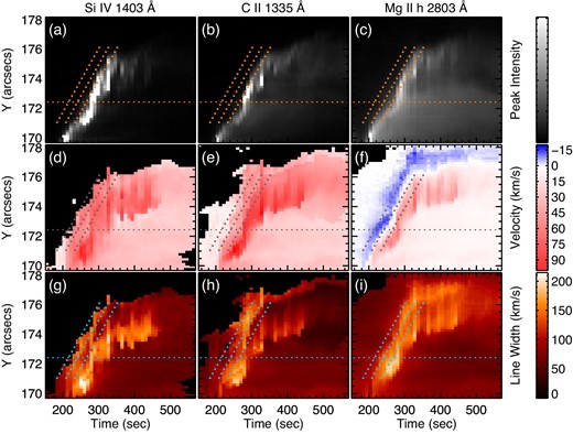
Space–time plots of (a)–(c) line peak intensity, (d)–(f) Doppler velocity, and (g)–(i) line width of the IRIS lines. Three diagonal-dotted lines are drawn at the same space and time on all the panels to make a comparison between different panels; each slope corresponds to an apparent velocity of 31 km s⁻¹. The detail of the location indicated by the horizontal-dotted line (y_slit = 172|${^{\prime\prime}_{.}}$|4) is shown in figure 7. The black areas in the panels (d)–(i) present the regions where the physical parameters cannot be derived due to their very weak intensity. We also show color bars for the three quantities on the right-hand side. Intensity plots are shown in logarithmic scale; lighter colors show the brighter value. (Color online)

Open in new tabDownload slide

Fig. 6.

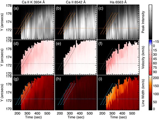
Same as figure 5, but for the DST lines. Three diagonal-dotted lines are drawn at the same space and time as those in figure 5. The detail of the location indicated by the horizontal-dotted line (y_slit = 172|${^{\prime\prime}_{.}}$|4) is shown in figure 8. Note that the DST observation began t = 242 s. (Color online)

Open in new tabDownload slide

Here, we focus on the evolution of the peak intensity, the Doppler velocity, and the line width from 171|${^{\prime\prime}_{.}}$|0 to 176|${^{\prime\prime}_{.}}$|2 in y_slit. (The evolution from 176|${^{\prime\prime}_{.}}$|2 to 178|${^{\prime\prime}_{.}}$|1 in y_slit is described in the last paragraph of this section.) The temporal variations of the three quantities at the pixels in the y_slit range were similar to each other, while the redshifts continued longer in the positions from 174|${^{\prime\prime}_{.}}$|0 to 176|${^{\prime\prime}_{.}}$|2 in y_slit. The spatial width of the region with the blueshift in the Mg ii h line was ∼ 700 km in the traveling direction. Recently, Xu et al. (2016) observed the dark feature in the He i 10830 Å line at the leading edge of the flare footpoints before the burst phase. The spatial width of the dark feature in their study (340–510 km) was smaller than that of the feature with the blueshift in this study, but both occurred at the leading edge of flare footpoints.

With figures 7 and 8, we take a closer look at the typical temporal variation of the three quantities at a pixel: the peak intensity, the line width, and the Doppler velocity at y_slit = 172|${^{\prime\prime}_{.}}$|4 (horizontal-dotted line in figure 5 and 6). At this location, the blueshift in the Mg ii h line was the largest among all of the pixels from 171|${^{\prime\prime}_{.}}$|0 to 176|${^{\prime\prime}_{.}}$|2 in y_slit. The blueshift that was larger than 5 km s⁻¹ lasted for 29 s with a maximum velocity of 14 km s⁻¹ (shown by the blue arrow in figure 7). During this period, the intensity of the Mg ii h was still small, but just started getting large. The line width became broader when the blueshift appeared in the Mg ii h line. After that, the large redshift in the Si iv, C ii, and Mg ii h lines lasted for 67 s, 29 s, and 10 s (e-folding time) with a maximum velocity of 62 km s⁻¹, 79 km s⁻¹, and 51 km s⁻¹, respectively. The intensity and the line width also increased together. The three quantities reached their maxima at almost the same time, as indicated by the red arrow, while the line width in the C ii line peaked 9.5 s earlier. As for the DST lines, when the observation started (purple arrow in figure 8), the blueshift in the Mg ii h line was almost over, and all the DST lines showed redshifts. At y_slit = 172|${^{\prime\prime}_{.}}$|4, the maximum velocity was 34 km s⁻¹, 15 km s⁻¹, and 46 km s⁻¹ for the Ca ii K, Ca ii 8542 Å, and Hα lines, respectively. Then, the Doppler velocities decreased in the three lines. The line widths varied similarly in the case of the line shifts. The brightening in the three DST lines peaked a little later and persisted longer than in the IRIS lines.

Fig. 7.

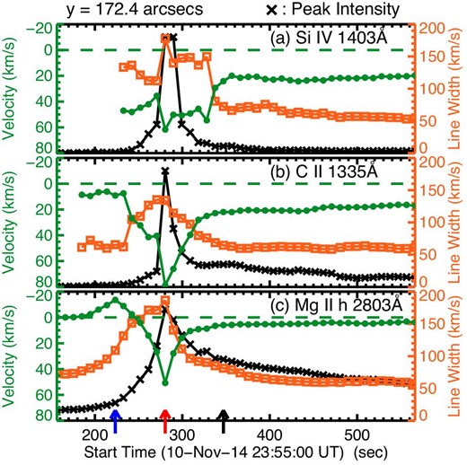
Temporal evolution of the peak intensity (black cross), the Doppler velocity (green circle), and the line width (orange square) in the IRIS lines at y_slit = 172|${^{\prime\prime}_{.}}$|4 on the IRIS slit. The vertical axes of the peak intensities are arbitrary. Negative velocity represents a blueshift, while positive velocity a redshift. The line width and velocity are not shown in the time period when the intensity was too weak to determine. Three arrows at the bottom indicate the same times when the spectra shown in the panels in figure 9 were taken. The blue and red arrows are the times of the minimum velocity (blueshift) (t = 223 s) and the maximum velocity (redshift) (t = 280 s) in the Mg ii h line, respectively. (Color online)

Open in new tabDownload slide

Fig. 8.

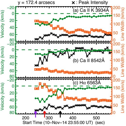
Same as figure 7, but for the DST lines. Three arrows indicate the times when spectra shown in the panels in figure 10 were taken. The purple arrow is the first time of the DST observation (t = 242 s). The red arrow is the time of the maximum velocity (redshift) in the Mg ii h line, and is the same as the red arrow in figure 7. (Color online)

Open in new tabDownload slide

The line profiles at the times indicated by the three arrows in figure 7 are shown in figure 9. From figures 7c and 9g–9i, we can recognize that the blueshift in the Mg ii h line was due to the weak enhancement in the blue wing with a moderate peak intensity and that the redshift was due to a strong enhancement in the red wing with a large peak intensity. In addition, as shown in figure 9g, the blue-side peak (h2v) was smaller than the red-side one (h2r). The Si iv (figures 9a–9c) and C ii lines (figures 9d–9f) show a strong enhancement in the red wing, particularly at t = 223 s and 280 s, respectively. Note that the profile shown in figure 9b was saturated. Figure 10 shows similar plots to figure 9, but for the DST lines at the times indicated by the three arrows in figure 8, with the reference and original profiles. In all of the DST lines at t = 248 s and 278 s, no blueshift was confirmed and strong emission, especially in the red wing, can be seen. These characteristics were similar at all positions from 171|${^{\prime\prime}_{.}}$|0 to 176|${^{\prime\prime}_{.}}$|2 in y_slit. Figure 11 shows the detail of the blueshift in the Mg ii lines from 171|${^{\prime\prime}_{.}}$|0 to 176|${^{\prime\prime}_{.}}$|2 in y_slit. In figure 11a, black plus signs show the distribution of the blueshift that was larger than 5 km s⁻¹ at the location from 171|${^{\prime\prime}_{.}}$|0 to 178|${^{\prime\prime}_{.}}$|1 in y_slit. Each of the thick plus signs among them indicates the time of the peak blueshift at each pixel of the location from 171|${^{\prime\prime}_{.}}$|0 to 176|${^{\prime\prime}_{.}}$|2 in y_slit, where the blueshift preceded the redshift. The thick and thin lines in figures 11b and 11c show respectively the average and five examples of the Mg ii h- and k-line-profiles at the positions indicated by the black and colored thick plus signs in figure 11a. As is the case with the profile in figure 9g, the averaged profile of the Mg ii h line had the enhanced blue wing and the small intensity of the blue-side peak (h2v) compared to the red-side peak (h2r), which was the typical shape among the blue-shifted line profiles. The Mg ii k line behaved in a similar manner to the Mg ii h (figures 11b–11c), while its intensity is larger and its blue wing is blended with another line. In the Mg ii h line, the mean velocity of the blueshift indicated by thick plus signs in figure 11 a was 10.1 km s⁻¹ with the standard deviation of 2.6 km s⁻¹. The mean duration of the blueshift (>5 km s⁻¹) at one pixel location was 28 s with a minimum and a maximum duration of 9 s and 48 s, respectively. Figure 11d shows an example of the temporal evolution of the Mg ii h line profiles at a specific location (y_slit= 173|${^{\prime\prime}_{.}}$|1; square signs in figure 11a): the transition from the blue-shifted profiles to the red-shifted profiles. The strong redshift and the red-wing enhancement were observed just after the moderate intensity with the blue-wing enhancement. This was the typical evolution of the Mg ii h and k profiles in the location from 171|${^{\prime\prime}_{.}}$|0 to 176|${^{\prime\prime}_{.}}$|2 in y_slit.

Fig. 9.

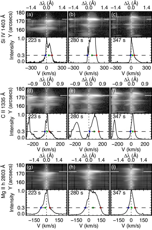
Spectral images and profiles of the IRIS (a)–(c) Si iv, (d)–(f) C ii, and (g)–(i) Mg ii h at t = 223 s, t = 280 s, and t = 347 s, corresponding to the times of three arrows in figure 7. In the upper portion of each panel, the space–wavelength plot in the vicinity of the flare kernel is shown. The original line profile at the spatial position y_slit = 172|${^{\prime\prime}_{.}}$|4 (indicated by the horizontal solid lines in the upper image) is shown in the lower portion of each panel. The peak intensity is normalized to unity and the horizontal axis is converted from the wavelength to the velocity. The threshold of the intensity to define the bisector (30% peak intensity) (dashed line) and the rest wavelength (dotted line) are shown. The blue and red dots indicate the positions of the two wing wavelengths at 30% peak intensity and the green dot shows the bisector wavelength of the two wings. Note that the intensity is saturated in panel (b) and the another C ii line appears in panels (d)–(f), in the shorter wavelength of the C ii 1335 Å. (Color online)

Open in new tabDownload slide

Fig. 10.

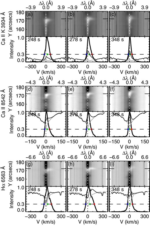
Spectral images and profiles of the DST (a)–(c) Ca ii K, (d)–(f) Ca ii 8542 Å, and (g)–(i) Hα at t = 248 s, t = 278 s, and t = 348 s, corresponding to the nearest times of three arrows in figure 8. In the upper portion of each panel, the space–wavelength plot in the vicinity of the flare kernel is shown. The lower portion of each panel shows the original line profile (thin black line), the reference line profile (thin gray line), and the difference profile obtained by subtracting the reference profile from the original one (thick black line) at the spatial position y_slit = 172|${^{\prime\prime}_{.}}$|4 (indicated by the horizontal solid lines in the upper region). The peak intensity of the difference profile is normalized to unity in each panel. Horizontal-dashed line and colored dots are the same as those in figure 9 but using the difference profile. Note that the intensities of the original and reference line profiles are shown on an arbitrary scale. (Color online)

Open in new tabDownload slide

Fig. 11.

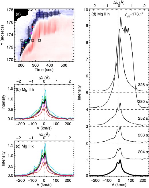
Details of the blueshift in the Mg ii lines at the location from 171|${^{\prime\prime}_{.}}$|0 to 176|${^{\prime\prime}_{.}}$|2 in y_slit, where the blueshift preceded the redshift. (a) Distribution of the blueshift in the Mg ii h line. Background is the same as in figure 5f. Plus signs indicate the time and location at which the blueshift of the bisector was larger than 5 km s⁻¹. Each thick plus sign shows the time when the blueshift reached a maximum at each location. Mg ii h- and k-line profiles at the positions of colored thick plus signs are shown in panels (b) and (c), respectively. Each square sign indicates the time and location of each Mg ii h line profile in panel (d). (b)–(c) Thick black line shows the average of the Mg ii (b) h- and (c) k-line profiles at the positions indicated by thick plus signs in panel (a), respectively. (d) An example of the temporal evolution of the Mg ii h line profiles at the positions indicated by the square signs in panel (a) (y_slit = 173|${^{\prime\prime}_{.}}$|1). Time passes from bottom up and the times are shown except the lowest profile, which is the same as the averaged one in panel (b). In panels (b)–(d), the vertical-dotted lines show the rest wavelength and the peak intensity of the averaged line profile of Mg ii h is normalized to unity. (Color online)

Open in new tabDownload slide

As we have confirmed, the intensity, the redshift, and the line width in all of the six lines had spatially and temporally good correlations with each other. The moving flare kernel was observed simultaneously with the increase of the Fermi HXR flux. Therefore, the variation of the three quantities would be involved in the variation of the energy input by electron beams (Fang et al. 1993). The maximum velocity of the redshift at y_slit = 172|${^{\prime\prime}_{.}}$|4 for each line was 62 km s⁻¹ (Si iv), 79 km s⁻¹ (C ii), and 51 km s⁻¹ (Mg ii h), 34 km s⁻¹ (Ca ii K), 15 km s⁻¹ (Ca ii 8542 Å), and 46 km s⁻¹ (Hα). These values were of the same order as the values in the previous reports (Ichimoto & Kurokawa 1984; Shoji & Kurokawa 1995; Liu et al. 2015).

Finally, we describe the evolution in the region of 176|${^{\prime\prime}_{.}}$|2 to 178|${^{\prime\prime}_{.}}$|1 in y_slit, which corresponds to the northern leading edge of the flare kernel in its decaying phase. In contrast with the region that we reported in previous paragraphs, the blueshift in the Mg ii h line in this region was not followed by any redshift. Instead, a rather persistent blueshift was observed in the Mg ii h line (see figure 5). The blue-shifted Mg ii h line profiles at y_slit >176|${^{\prime\prime}_{.}}$|2 had a lower intensity than those at y_slit < 176|${^{\prime\prime}_{.}}$|2. In other lines, the intensities in this region were small as well. We discuss this long-lasting blueshift in subsection 5.6.

5 Discussion

5.1 Observational results related to the blueshift in the Mg ii lines

We discovered the blue-wing enhancement of the Mg ii h and k lines prior to the large intensity and redshift. The blueshift in the wing amounts to 10.1 ± 2.6 km s⁻¹, which lasted for 9–48 s or for 28 s on average in the Mg ii h line. It is also found that the blue-side peaks (h2v and k2v) were weaker than the red-side ones (h2r and k2r) in the Mg ii h and k lines during this period. We discuss two scenarios for such a blueshift: the cool-downflow scenario in subsection 5.2 and the cool-upflow scenario in subsections 5.3, 5.4, and 5.5. In addition, we observed a long-lasting blueshift that was not followed by any large redshift and intensity. Note that we could not confirm any filament-like motion around the location where the blue-wing enhancements were observed.

5.2 Discussion of the blueshift: the cool-downflow scenario

First, let us think about a possibility that a downward motion of chromospheric plasma generates the blue asymmetry. Heinzel et al. (1994) proposed a model in which the upper chromospheric layer moving downward absorbs the radiation of the red-side peak of emission in the Hα line formed in deeper layer, thus lowering its intensity compared to the blue-side one. Kuridze et al. (2015) calculated the chromospheric line profiles, and showed that the blue asymmetry can occur in the Hα line, which is due to the shift of the maximum opacity of the overlaying layer to longer wavelengths. However, in such cases, the intensity of the red-side peak is lower than that of the blue-side one, while in our observation the red-side peak was higher than the blue-side one in the Mg ii h and k lines. Hence, this scenario cannot explain the observed feature of the Mg ii h and k lines.

5.3 Discussion of the blueshift: the cool-upflow scenario

Secondly, Canfield et al. (1990) discussed that an upward motion of chromospheric plasma can cause the blue asymmetry when high-energy electrons rush into the deep chromosphere in the early phase of the flare. Although in their study the blueshift in the Hα line occurred when the intensity level maximized, the blueshift in the Mg ii h line in our observation lasted for 9–48 s at each pixel before the largest intensity and redshift. We present a scenario for our observation in figure 12, which is a cartoon of the temporal variation of the plasma dynamics at a flare footpoint; high-energy electrons penetrate into the deeper layer, and the plasma is heated to orders of magnitude of 10⁶⁻⁷ K. Then, the chromospheric cool plasma above the expanded plasma is lifted up, which can be observed as a blueshift in chromospheric lines until the radiation from the condensation region becomes too strong. This scenario is partially implied in one-dimensional hydrodynamic simulations of flaring loops by thick-target heating (Nagai & Emslie 1984; Allred et al. 2005; Kennedy et al. 2015; Rubio da Costa et al. 2015b). In Allred et al. (2005), the cool (Log T[K] = 4.5–4.7), dense plasma is moving upward above the hot (Log T[K] = 6.0–6.5) plasma during the explosive phase of both the moderate and strong heating cases, while the radiation from the chromospheric condensation region seems to be already strong in this phase. In Kennedy et al. (2015), the non-thermal electron beam heating causes a region of high-density cool (Log T[K] = 4.0–4.5) material propagating upward (∼100 km s⁻¹) through the corona during the explosive phase. Then, the temperature of this material rapidly increased because the energy input by non-thermal electrons and by thermal conduction was too large to be radiated away. We suppose that in a specific condition, flare heating can balance with radiative cooling in such a cool dense plasma, and the material can survive for a longer time. The blue-wing enhancement in the Mg ii h line observed in our study may be attributed to such a cool upflow above the expanding hot plasma, which is attributed to high-energy electrons. Actually, the blueshift in the Mg ii h line occurred in the second burst with an increase of the time derivative of the GOES SXR flux and Fermi HXR flux (figure 2), which is a proxy of the energy input by high-energy electron beams.

Fig. 12.

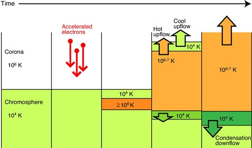
Schematic cartoon of the one-dimensional cool-upflow scenario we discuss in this study. The deep penetration of non-thermal electrons into the chromosphere causes an upflow of the chromospheric-temperature (cool) plasma lifted up by the expanding (hot) plasma, before the strong emission in the chromospheric lines from the downward-moving condensation region. (Color online)

Open in new tabDownload slide

5.4 Cloud modeling based on the cool-upflow scenario

Fig. 13.

(a) Cloud-model calculation of the Mg ii h line profile with the values of free parameters: V_LOS = −40 km s⁻¹, V_turb = 40 km s⁻¹, τ₀ = 0.5, and α = 0.6. The synthesized line profile well reproduces the averaged profile from the observation. The calculated line profile I (Δλ) is shown in the orange solid line, the background intensity I₀(Δλ) in the green-dotted line, the two terms in the radiative transfer equation I₀exp[−τ(Δλ)] and S{1 − exp[−τ(Δλ)]} in the blue-colored dash-dotted line and red-colored dot-dot-dot-dashed line, respectively. The intensity is normalized by the background peak intensity, I₀(Δλ = 0). (b) Comparison of the calculated [orange thinner solid line, which is the same as in the panel (a)] and the observed (black thicker solid line) profile of the Mg ii h line. The background intensity, I₀(Δλ), is also shown by the green-dotted line. The vertical-dashed line shows the position of the rest wavelength corresponding to Δλ = 0. The solid vertical line indicates the wavelength position of the emission from the moving cloud. Its line-of-sight velocity is V_LOS = 40 km s⁻¹. Note that the bisector method generally leads to smaller shifts compared to the cloud-model fitting (The typical blueshift corresponded the velocity of 10.1 ±  2.6 km s⁻¹ by the bisector method in the observation). (Color online)

Open in new tabDownload slide

It is true that we did not perform the full non-LTE (local thermodynamic equilibrium) modeling of the Mg ii line profiles, which can be done in a following paper. Therefore, we do not exclude other possibilities. However, the cloud model, itself, represents a formal solution of the non-LTE transfer equation, assuming a simple model with constant quantities within a moving layer. In comparison with the observed profiles, the cloud model provides a reasonable estimate of the flow velocity and the line width, along with two other quantities, which are the line source function and the line center optical thickness. The emission from the moving cloud produces the blue-wing enhancement, and the absorption by the cloud causes a lowering of the blue-side peak. For further understanding, detailed non-LTE modeling will be needed to compute other quantities. This will then require a model of the temperature and density structure. Such models have been recently produced using the hydrodynamical code (T. Nakamura et al. in preparation), and preliminary non-LTE modeling based on selected-time snapshots, indeed, leads to qualitatively the same Mg ii profiles as observed (P. Heinzel 2017 private communication).

5.5 Consistency of the cool-upflow scenario with observational results in various lines

Next, why was not the blueshift observed in other lines at the time when it appeared in the Mg ii h line? Concerning the DST lines, one possibility is that the region with the blue-wing enhancement (spatial scale ∼1″) was not resolved by the ground-based DST observation because of the seeing effect (∼2″). Another possibility is due to opacity differences: if we assume that the VAL-C atmosphere (averaged quiet Sun model: Vernazza et al. 1981) is an initial model, and pay attention to the 10700 K plasma, then the opacity of the Mg ii h line is estimated to be about 14 times larger than that of the Hα line. In addition, the opacity of the Mg ii h line is known to be larger than that of the Ca ii K line and also that of the Ca ii 8542 Å line (Leenaarts et al. 2013). Therefore, it is possible that the cool upflow is seen in the Mg ii h line, but not in the Ca ii K, Ca ii 8542 Å, and Hα lines. On the other hand, the opacity of the C ii 1335 Å line is similar to that of the Mg ii h line (Rathore et al. 2015). Indeed, the blue-side peak was typically smaller than the red-side peak in the C ii 1335 Å line, but no blue-wing enhancement was observed in our study. This can be interpreted as follows: the difference in the peak intensities can be understood based on the same model as that of the Mg ii h line. However, the source function of the upward-moving cloud might be too small to cause a blue-wing enhancement in C ii 1335 Å. Finally, the Si iv 1403 Å line forms at transition-region temperatures of around 10⁵ K, and thus is optically thin at 10⁴ K. The upward-moving cool cloud might be transparent in the Si iv 1403 Å line.

5.6 Interpretation of the long-lasting blueshift

While a bluesift was followed by a redshift from 170|${^{\prime\prime}_{.}}$|0 to 176|${^{\prime\prime}_{.}}$|2 in y_slit in the Mg ii h line, a long-lasting blueshift without a clear redshift was observed from 176|${^{\prime\prime}_{.}}$|2 to 178|${^{\prime\prime}_{.}}$|1 in y_slit. This cannot be explained by the cool-upflow scenario discussed above, where a cool plasma is lifted up by an expanding hot plasma. The blue-shifted Mg ii h line profiles at y_slit > 176|${^{\prime\prime}_{.}}$|2 had a lower intensity than those at y_slit < 176|${^{\prime\prime}_{.}}$|2. This means that the energy flux at y_slit > 176|${^{\prime\prime}_{.}}$|2 was so small, and heating was weak, which resulted in smaller kinetic energy of the downward flow. Thus, the downward velocity and the downward compression would have been weak, and no bright condensation downflow would be observed. On the other hand, it is reasonable that any cool upflow would be associated with such a small energy flux. There are possible interpretations for both cases with the small energy input in the deeper chromosphere and the middle or upper chromosphere. A small energy input in the deeper chromosphere could lead to local heating, causing any gas pressure increase to generate a shock wave, which would drive cool upflow when it crosses the transition layer (Osterbrock 1961; Suematsu et al. 1982). In this case, the transition region would move upward, which would result in cool upflow without any expanding hot plasma. If a small energy input is given in the middle or upper chromosphere to increase the gas pressure to a few times the initial value, then the gas pressure gradient force would accelerate the cool plasma upward (Shibata et al. 1982). Also, in this case the cool upflow would not be associated with any expanding hot plasma.

5.7 Summary and future work

We performed coordinated observations of NOAA AR 12205, which produced a C-class flare on 2014 November 11, with IRIS and DST at Hida Observatory. Using spectral data in the Si iv 1403 Å, C ii 1335 Å, and Mg ii h and k lines from IRIS and the Ca ii K, Ca ii 8542 Å, and Hα lines from DST, we investigated the temporal, spatial evolution around the flare kernel during the flare. The flare kernel apparently moved along the IRIS slit. In the Mg ii h line, the leading edge of the flare kernel showed an intensity enhancement in the blue wing, and a small intensity of the blue-side peak (h2v) compared to the red-side one (h2r). Then, a drastic change in the intensity of the red wing occurred. The blueshift lasted for 9–48 s with a typical speed of 10.1 ±  2.6 km s⁻¹, which was followed by a strong redshift with a speed of up to 51 km s⁻¹, detected in the Mg ii h line. The strong redshift was a common property for all of six spectral lines used in this study, but the blueshift prior to it was found only in the Mg ii lines. Cloud modeling of the Mg ii h line suggests that the blue-wing enhancement with such a peak difference could have been caused by a chromospheric-temperature (cool) upflow. We discuss a scenario in which an upflow of cool plasma is lifted up by expanding (hot) plasma owing to the deep penetration of non-thermal electrons into the chromosphere. In addition, a long-lasting blueshift was also observed in the Mg ii h line, which was not followed by any large redshift and intensity enhancement. This occurred at the northern leading edge of the flare kernel in its decaying phase. Such a long-lasting blueshift can be explained by the cool upflow caused by such a small energy flux into the lower atmosphere where expanding hot upflow would not be produced.

The chromospheric lines used in this study are formed under the non-LTE condition. The observed line profile is influenced by the three-dimensional radiative field, depending on the temperature and the density structure. In the case of no velocity field, the intensities in the line core and wings would reflect information about the higher and lower levels of the atmosphere, respectively, since the absorption coefficient has its maximum in the line core and is smaller in the wings. In addition, there are large velocity gradients during solar flares. Therefore, it is not so simple to diagnose the velocity field at a certain height based on spectral line profiles. Modeling of the flaring atmosphere and synthesizing chromospheric line profiles has been conducted so far (e.g., Nagai & Emslie 1984; Allred et al. 2005; Rubio da Costa et al. 2015a, 2015b, 2016; Rubio da Costa & Kleint 2017). Our result concerning the blueshift in the Mg ii lines will restrict further modeling. There would be both cases of flaring regions with and without any signature of a blueshift in the chromospheric lines. Even at a single location, the chromospheric response to flares would differ among different observing lines. The initial condition and the energy input may affect the evolution of cool upflow significantly, and the spectra would also change sensitively due to the surrounding environment. More studies are needed in the future to clarify what causes these differences, and to understand the heating mechanism of the flaring chromosphere based on spectroscopic observations.

Acknowledgement

A.T. would like to thank Dr. Wei Liu and Dr. Fatima Rubio da Costa for helpful discussions. IRIS is a NASA small explorer mission developed and operated by LMSAL with mission operations executed at NASA Ames Research Center and major contributions to downlink communications funded by ESA and the Norwegian Space Centre. SDO is part of NASA’s Living With a Star Program. This work was partly carried out on the Solar Data Analysis System operated by the Astronomy Data Center in cooperation with the Hinode Science Center of NAOJ. This work was supported by JSPS KAKENHI Grant Numbers, JP17J07733 (PI: A.T.), JP16K17663 (PI: T.J.O.), JP17K14314 (PI: T.K.), JP15K17772 (PI: A.A.), JP15H05814 (PI: K.I), JP16H03955 (PI: K.S.), and JP25220703 (PI: S. Tsuneta). P.H. acknowledges support from the Czech Funding Agency through the grant No. 16-18495S and from Kyoto University during his stay in Japan.

References

Author notes