


Abstract
A new sideband separation method was developed for use in millimeter-/submillimeter-band radio receivers using a novel waveguide frequency separation filter (FSF), which consists of two branch line hybrid couplers and two waveguide high-pass filters. The FSF was designed to allow the radio frequency (RF) signal to pass through to an output port when the frequency is higher than a certain value (225 GHz), and to reflect the RF signal back to another output port when the frequency is lower. The FSF is connected to two double sideband superconductor-insulator-superconductor (SIS) mixers, and an image rejection ratio (IRR) is determined by the FSF characteristics. With this new sideband separation method, we can achieve good and stable IRR without the balancing two SIS mixers such as is necessary for conventional sideband-separating SIS mixers. To demonstrate the applicability of this method, we designed and developed an FSF for simultaneous observations of the J = 2–1 rotational transition lines of three CO isotopes (12CO, 13CO, and C18O): the 12CO line is in the upper sideband and the others are in the lower sideband with an intermediate-frequency range of 4–8 GHz at the radio frequency of 220/230 GHz. This FSF was then installed in the receiver system of the 1.85 m radio telescope of Osaka Prefecture University, and was used during the 2014 observation season. The observation results indicate that the IRR of the proposed receiver is 25 dB or higher for the 12CO line, and no significant fluctuation larger than 1 dB in the IRR was observed throughout the season. These results demonstrate the practical utility of the FSF receiver for observations like extensive molecular cloud surveys in specified lines with a fixed frequency setting.
1 Introduction
In radio astronomy, superconductor–insulator–superconductor (SIS) mixers are widely used for millimeter-/submillimeter-band heterodyne receivers, because they have a very low noise temperature of approximately several times the quantum limit (e.g., Ellison et al. 1989; Ogawa et al. 1990; Monje et al. 2007; Kerr et al. 2013). The SIS mixer is intrinsically a double-sideband (DSB) mixer, which merges both upper- and lower-sideband (USB and LSB) signals into a single intermediate frequency (IF) output signal. However, single-sideband (SSB) or sideband-separating (2SB) receivers are highly desirable for spectral line observations in radio astronomy and remote-sensing applications at millimeter/submillimeter wavelengths. The merit of the sideband separation receiver is not only in rejecting the contamination of spectral lines, but also in reducing the atmospheric noise contribution coming from the other sideband.
For this reason, 2SB SIS mixer receivers, which consist of two well-balanced SIS mixers, have been well developed (e.g., Asayama et al. 2004; Vassilev et al. 2004), and used for many radio telescopes including the Atacama Large Millimeter/submillimeter Array (ALMA) (Band 4: Asayama et al. 2014; Band 5: Billade et al. 2009; Band 6: Kerr et al. 2004; Band 7: Claude 2003; Band 8: Kamikura et al. 2006), and the 60 cm telescope receiver (Nakajima et al. 2007), the single-beam receiver T100 (Nakajima et al. 2008), the two-beam receiver TZ (Nakajima et al. 2013), and also the four-beam receiver system on the 45 m telescope (FOREST: Minamidani et al. 2016).
However, this type of 2SB SIS mixer has some intrinsic problems. First, it requires two SIS mixers with nearly equivalent frequency characteristics (noise temperature, conversion gain, and so on) to obtain a sufficient image rejection ratio (IRR), which represents the degree to what the receiver rejects the power of the opposite sideband signal, and sometimes it is difficult to find one pair of appropriate SIS mixers. Second, the two SIS mixers composing a pair easily get out of balance, and suffer degradation in the frequency characteristics, due to short-term fluctuations and a long-term drift during operations with various tuning parameters of the SIS mixer, such as bias voltage and local oscillator (LO) signal power. Third, the IRR largely depends on the frequency, sometimes showing a poor ratio in a certain frequency range.
Stability of the IRR is especially important for long-term observations, such as monitoring the abundance of specific molecules in the atmosphere (e.g., Nagahama et al. 2007; Nakajima et al. 2010; Ohyama et al. 2016), which requires highly accurate intensity calibrations. Therefore, researchers performing long-term observations have usually been reluctant to use 2SB SIS mixer receivers, because their IRR instability makes the SIS mixer unsuitable for long-term observations. For example, Ohyama et al. (2016) showed that the scaling factors for the intensity calibration seemed to be fluctuating during the long-term monitoring of ozone abundance, which can be at least partially explained by the IRR instability.
To solve this issue, Asayama et al. (2015) developed a new method for the image rejection filter. This filter acts as a high-pass filter under the following situation: when we set an LO frequency of 104 GHz and IF of 4–8 GHz, the LSB signals (96–100 GHz) are rejected by the internal absorbers, and thus the USB signals (108–112 GHz) can be observed with a high IRR (∼25 dB). This filter was installed in the receiver used for remotely monitoring the ozone spectrum, and a new SSB receiver with a very high and stable IRR was successfully realized.
In this paper we report on the new sideband separation receiver containing a circuit called the frequency separation filter (FSF), which is an advanced version of Asayama et al. (2015)'s SSB filter. The FSF can divide an input signal into two frequency bands. The high-frequency band passes through the internal high-pass filter and the low-frequency band is reflected. If we assign the USB and LSB of the mixer receiver into those two bands, respectively, the circuit can be used to separate the USB and LSB signals with a good and stable IRR, which is determined by the properties of the internal high-pass filters. The functional principle of the FSF is described in section 2.
Furthermore, in order to establish a novel CO-molecular-line receiver with a high IRR based on the FSF technique, and also to demonstrate its usefulness through actual astronomical observations, we developed a receiver system by integrating the proposed FSF in the 220/230 GHz band (hereafter referred to as the 220/230 GHz FSF), and then applied it to the simultaneous observation of the J = 2–1 rotational transition lines of three CO isotopes (12CO, 13CO, and C18O). The detailed design and measurements of the 220/230 GHz FSF are described in section 3, the installation into a 1.85 m radio telescope is discussed in section 4, and the observation results using the proposed receiver are shown in section 5.
2 Principles of the proposed frequency separation filter
2.1 Backward effect of the branch line coupler
The waveguide-type branch line coupler (BLC) is a well-known four-port waveguide circuit used as a quadrature hybrid coupler (e.g., Schiek et al. 1974; Andoh et al. 2003). An input signal to the 3 dB BLC is divided into two, and then delivered to two output ports, port 3 and port 4, with almost the same magnitude, having a 90° phase difference between them, as shown in figure 1a. In this case, port 2 does not output any signals.
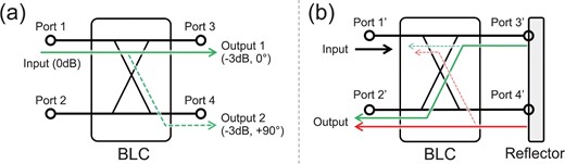
(a) Schematic of a four-port quadrature hybrid coupler (BLC). (b) Schematic of the backward effect of a BLC with output ports 3 and 4 replaced by an ideal reflector. (Color online)
There is another feature for the BLC when we put reflection walls at both port 3 and port 4, as shown in figure 1b: all the input signal into port 1΄ is delivered to port 2΄ without any return signal to port 1΄. This is because the two reflected signals from port 3΄ and port 4΄ are canceled at port 1΄: the reflected signal from port 4΄ has a 180° phase difference compared with that from port 3΄ at port 1΄ (e.g., Navarrini & Nesti 2009; Navarrini et al. 2010). Therefore, all the input signal goes to port 2΄ in this case. Hereafter, we call this effect the “backward effect” (BWE).
2.2 Sideband separation with FSF
The FSF developed in the present study is composed of two BLCs and two waveguide high-pass filters (HPFs): each device has the same frequency characteristics, as shown in figure 2a. The behavior of the FSF depends on the frequency of the input signal. When the frequency of the input signal is higher than the cutoff frequency of the internal HPFs, all the signal goes to port 4. When the input frequency is lower than the cutoff frequency, all the input signal goes to port 2. Therefore, if we set the USB frequency passing the HPFs and the LSB at a lower-than-cutoff frequency, the USB signal goes to port 4 and the LSB to port 2, so that the FSF separates the sidebands. Port 3 needs to be terminated by a 4 K absorption load. This is necessary for making BLC #2 work properly as a four-port hybrid coupler. This also works as a cold-load termination for the image band of both LSB and USB mixers. The image termination occurs by the signal transmission through the HPF for the LSB mixer at port 2, and by the signal reflection at the HPF for the USB mixer at port 4.
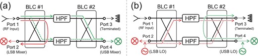
(a) Schematic of the FSF using two BLCs and two HPFs. The green lines (from port 1 to port 4) show the transmission of signals that can pass the HPFs. The red line (from port 1 to port 2) shows the transmission of signals that cannot pass the HPFs. (b) Schematic of LO leakage transmission on the FSF. The red lines show the transmission of the LO leakage passed by the HPFs from the LSB mixer’s LO coupler. The green line shows the transmission of LO leakage that cannot pass the HPFs from the USB mixer’s LO coupler. In both cases, the leakages reaching port 3 would be terminated by the absorption load. (Color online)
Furthermore, managing the LO power leakage from the LO coupler is important in ensuring that the stable LO power is applied to the mixer. For the FSF, this depends on the LO frequency relative to the cutoff frequency of the internal HPFs. The leakages are terminated by the 4 K load in following two cases, as shown in figure 2b:
When the LO frequency from port 2 is high and the leakage power passes the HPFs, it reaches port 3, and then would be terminated.
When the LO frequency from port 4 is low and the leakage power is reflected by the HPFs, it is transmitted to port 3 through the BWE, and then is terminated.
In the other cases, the LO leakage is transmitted to port 1 and is emitted to the antenna by the feed horn, which is the same as a normal millimeter/submillimeter receiver without the FSF.
The advantages of the proposed receiver using the FSF, hereafter referred to as the 2SBF-Rx, are summarized as follows:
There is no need for a balance between the two SIS mixers, as the two SIS mixer receivers can be operated independently. This allows the SIS mixers to be operated at their full performance, without making a compromise for the purpose of balancing.
The 2SBF-Rx can achieve a high IRR with no fluctuation, because the sideband separation occurs in solid waveguide circuits.
The conventional 2SB SIS mixer receiver needs the RF 90° and IF 90° hybrid couplers, and also two coaxial cables to connect two SIS mixers and the IF hybrid, as shown in figure 3a (for details see Asayama et al. 2004; Nakajima et al. 2007). The 2SBF-Rx requires significantly fewer components. An FSF is simply needed to connect two SIS mixers, as shown in figure 3b: this makes the fabrication and installation much easier.
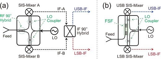
Schematics of a conventional receiver with 2SB SIS mixers (a), and the proposed 2SBF-Rx (b). (Color online)
The intrinsic disadvantage of the 2SBF-Rx is that the RF band is fixed by the design of the FSF, which means that the FSF must be replaced to change the frequency setting of the observation. However, its high IRR and stability are quite attractive, and it is thus suitable for survey-type observations with a fixed target frequency.
3 Design and measurement of 220/230 GHz frequency separation filter
3.1 Frequency design for observations of 12CO, 13CO, and C18O (J = 2–1) at 230 GHz
The rotational transition lines of CO are commonly observed in radio astronomy by a method of tracing interstellar gas (e.g., Dame et al. 1987; Heyer & Dame 2015; Onishi et al. 1996). The J = 2–1 lines of three CO isotopes, 12CO, 13CO, and C18O, are often observed simultaneously to investigate the physical properties and kinematics of target molecular clouds (e.g., Sakamoto et al. 1995; Yoda et al. 2010). The rest frequencies of these isotopes are 230.538, 220.399, and 219.560 GHz, respectively. Sideband-separating receivers with LO frequency ∼225 GHz have been widely used for these simultaneous observations (figure 3a). In this case, the three lines are converted into the frequency range of 4.5–5.5 GHz of the IF frequency, 12CO in the USB, and 13CO and C18O in the LSB. The low IRR results in line contamination between the two sidebands; in particular, 12CO and 13CO lines are quite strong, so that they appear in each opposite sideband with a significant intensity. With a typical 12CO antenna temperature of ∼10 K, the IRR should be better than 20 dB to reliably detect weak molecular lines of ∼0.1 K in the lower sideband.
The FSF can be used to separate the USB and LSB signals by selecting an appropriate cutoff frequency of the internal HPFs. We designed the HPFs so that signals with a frequency higher than 228 GHz pass through and frequencies lower than 222 GHz are reflected. Each waveguide circuit was designed with the commercial finite element software HFSS, which is a simulator that solves Maxwell's equations using the three-dimensional finite element method. All dimensions were optimized by manual parametric sweep analysis at a dimensional precision of 10 μm, to achieve two goals around the three CO lines: (1) the input return loss of the FSF is better than −15 dB; (2) the IRR calculated from the transmission toward each sideband signal's output port is better than 20 dB.
3.2 Design of the branch line coupler
In the design of the waveguide-type BLC, the number of branches is an important factor controlling its bandwidth, coupling ratio, and other characteristics. For designing the 220/230 GHz FSF, the observation band is only fixed for the CO lines, so that the bandwidth is not required to be very broad. Thus, we set the number of branches at five, which is a reasonable number for the design and manufacture of the circuit.
Figure 4a shows the simulation model of the designed BLC. Two WR-4.3 parallel waveguides were used to match the 230 GHz band SIS mixer and the other components. Figure 4b shows the simulated S-parameters of the designed BLC: the input return loss (S11), the port isolation (S21), and the coupling ratios of the main and side waveguides (S31 and S41, respectively). According to the plots of S31 and S41, the designed BLC has a coupling ratio of 3 dB ± 0.2 dB for 215–235 GHz, which is suitable for the observation of the CO isotope transition lines.
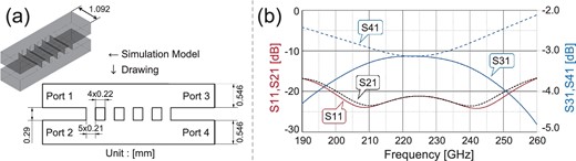
(a) Schematics of the designed BLC and simulation model, and (b) its simulated performance. (Color online)
3.3 Design of 230 GHz high-pass filter
For the HPF, we adopt a waveguide HPF characterized by the waveguide cutoff frequency in order to simplify the manufacturing process. Figure 5a shows the simulation model and the dimensions of the 230 GHz HPF for the parametric sweep at different values of the dimension HPY3, which is defined as the length of the narrowest part of the waveguide. In this simulation the other dimensions are fixed, including the middle-sized waveguide sections used as the stepping impedance transformer.
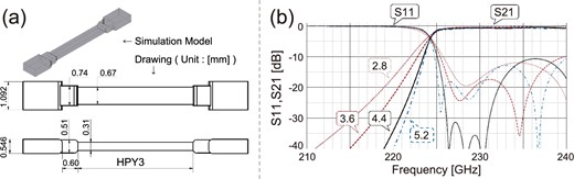
(a) Schematics of the parametric sweep simulation model, and (b) its simulated transmission performance, which calculated the transmission performance of a simple waveguide 230 GHz HPF at four different values of HPY3. (Color online)
The simulation results shown in figure 5b indicate that when HPY3 is not sufficiently large, the attenuation capabilities on the transmission (S21) in the cutoff band are weak, and the return loss (S11) is determined by the resonance nature of the waveguide. As shown figure 5b, S11 for HPY3 = 4.4 mm is under −30 dB at 226–231 GHz, smaller than the others, and S21 for HPY3 = 4.4 mm is smaller than −30 dB under 221 GHz. These parameters dominantly determine the IRR of FSF, and 20 dB or more IRR at the CO band is required for 220/230 GHz FSF; hence, HPY3 was set to 4.4 mm.
3.4 Design of 220/230 GHz frequency separation filter
Using the BLC and HPF described above, a 220/230 GHz FSF was designed. The components were connected as shown in figure 2, and several dimensions were optimized again based on the results of a parametric sweep.
Figure 6 shows the final simulation model and its simulated S-parameters. In figure 6b, S11 is the input return loss; S22 and S44 are the output port return losses; and S21 and S41 are the transmission efficiencies from the input port to the LSB and USB output ports, respectively.
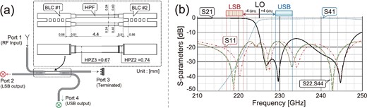
(a) Overview of the simulation model of the 220/230 GHz FSF, and (b) its simulated performances. (Color online)
As shown in figure 6b, input signals in the LSB band (217–221 GHz) are transmitted to the LSB output (port 2) with very low losses, and are not transmitted to the USB output (port 4) at all (less than −25 dB); the insertion loss S21 is approximately 0.40 dB at 220.4 GHz, including the ohmic loss of 0.34 dB for the assumed surface material (aluminum alloy A6063-T5), whose bulk conductivity is 3.3 × 10⁷ S m−1 at 300 K. The input signals in the USB band (229–233 GHz) are also transmitted to the USB output with an approximately 0.70 dB insertion loss, including 0.55 dB for the 300 K ohmic loss, and are not transmitted to the LSB output (less than −15 dB). These facts mean that the IRR of this FSF is better than 15 dB in the full IF band, and better than 20 dB for the observation of the rotational transition lines of the three CO isotopes.
3.5 Measurement results of manufactured frequency separation filter
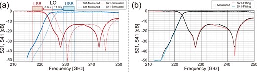
We manufactured a test piece of the FSF and measured the performance in order to confirm the FSF design. Figure 7a shows the measured S-parameters using a WR-3.4 vector network analyzer (VNA) extension module. The frequency range of this module is above 218 GHz, and thus the plot of the measured S41 values from 210 to 218 GHz demonstrates that they were below the noise floor of the WR-3.4 module.
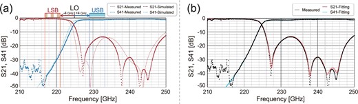
(a) Measured performance of the 220/230 GHz FSF. The red and blue lines show the transmission efficiencies from the input port to the LSB and USB output ports, respectively. The dots show the measurement results, and the dashed lines show the simulated performance, as in figure 6b. (b) Results of additional simulation of the 220/230 GHz FSF with different dimensions to consider the machining error. The black dots show the measurement results, and the red and blue lines show the LSB and USB outputs of the additional simulation, respectively, which accurately reproduced the measured performance. (Color online)
At all other frequencies considered, there were slight differences between the designed and measured S-parameters. After investigation of the differences, we found that they were attributed to machining errors. Therefore, we conducted an additional simulation with different device dimensions to fit the calculated performance with the measured results. The simulation can reproduce the measured results above, as shown in figure 7b; for the best fit, the dimensional parameters HPZ2 and HPZ3, which are the widths of the medium-width and the narrowest part of the HPF waveguide respectively, as shown in figure 6a, were shifted from 0.7400 to 0.7525 mm and from 0.6700 to 0.6682 mm, respectively.
When manufacturing the FSF, the FSF circuit was divided into two half-blocks to mill the waveguide, so that the depth machining error is doubled for the waveguide long-side dimensions. Therefore, the fitting results indicate that the machining error of manufactured devices for each part was less than 10 μm.
4 Installation of 220/230 GHz frequency separation filter in the 1.85 m telescope
The 220/230 GHz 2SBF-Rx has been installed in the 1.85 m telescope of Osaka Prefecture University (OPU). This millimeter/submillimeter radio telescope with a main reflector of 1.85 m in diameter was developed by the Radio Astronomy Group of OPU. It was also installed in the Nobeyama Radio Observatory of the National Astronomical Observatory of Japan (NRO/NAOJ) in 2007, and were used to simultaneously observe the J = 2–1 spectral lines of three CO isotopes with an approximately 10 dB IRR, which was determined by a conventional sideband separation receiver (Onishi et al. 2013; Shimoikura et al. 2013; Nishimura et al. 2015). Thus, this telescope is in a reasonable environment to demonstrate the performance of the proposed sideband separation receiver.
To install the 220/230 GHz FSF into the compact low-temperature (4 K) stage of the receiver cryostat for the 1.85 m telescope, an integrated waveguide circuit was newly developed. Figure 8 shows a photograph of a manufactured half-block of the integrated circuit, which includes the 220/230 GHz FSF circuit, two −17 dB LO signal couplers, and a 3 dB LO signal divider. The 220/230 GHz FSF also has four terminal ports with inserted radio wave absorbers of approximately −30 dB return losses: one is the terminated port of the FSF circuit, and the others are for LO signal absorption.
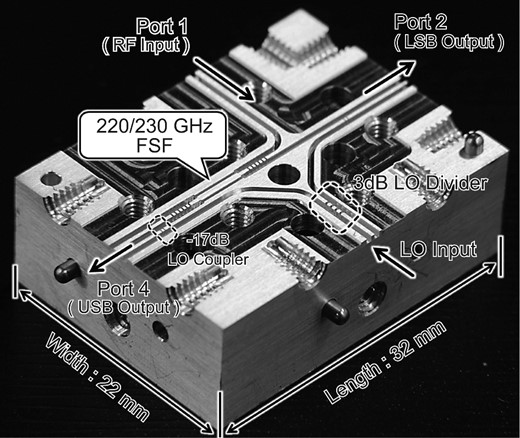
A photograph of the half-block of the integrated 220/230 GHz FSF.
The measured performances of this integrated 220/230 GHz FSF are shown in figure 9a, which were obtained under the same conditions as those in figure 7a. These results show that there is a band shift of approximately −2.5 GHz near 230 GHz, so the fitting simulations were conducted again to investigate the cause of this shift in the same manner as described in subsection 3.5. The best-fit simulation result shown in figure 9b indicates that these band shifts can be explained by the parameter HPZ2 shifted from 0.760 to 0.773 mm, and HPZ3 from 0.6660 to 0.6738 mm, respectively. These machining errors were expected to be canceled by the thermal contraction of the waveguide circuit at 4 K cooling: the shrinkage ratio of A6063-T5 from 300 K to 4 K is approximately 0.5%, and the estimated amount of the band shift was approximately +1.2 GHz near 230 GHz.
(a) Measured performance of the integrated 220/230 GHz FSF. The red S21 and blue S41 lines show the transmission from the input port to the LSB and USB output ports, respectively. The dots show the measurement data, and dashed lines show the simulated performance. (b) Fitting analysis results obtained in the same manner as in figure 7b for the integrated 220/230 GHz FSF. (Color online)
Furthermore, the measured insertion loss on S21 at 220.40 GHz is 1.04 dB, and that on S41 at 230.55 GHz is 1.11 dB. The measurement was conducted at 300 K, and these measured insertion losses include the estimated ohmic loss of 0.75 dB at 300 K; however, the ohmic loss is expected to be reduced to ∼0 at 4 K. The increase of TRX-SSB due to the FSF is thus estimated to be ∼5 K if we take into account the reduced ohmic loss at 4 K and the single-sideband receiver noise temperature TRX-SSB of ∼60 K.
This integrated 220/230 GHz FSF was installed into the 1.85 m telescope receiver system; a photograph of the installed 2SBF-Rx is shown in figure 10. This 4 K cooled receiver has a waveguide circular polarizer to separate left- and right-handed circular polarization components (Hasegawa et al. 2017), two integrated 220/230 GHz FSFs, two LO inputs, and four SIS mixers. The measured receiver noise temperatures, TRX-SSB, were ∼65–90 K, and the system noise temperatures including the atmosphere were 170–230 K at the frequent atmospheric optical depth τ ∼ 0.20.
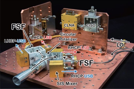
A photograph of the 220/230 GHz 2SBF-Rx installed into the 1.85 m telescope. (Color online)
5 Observation results
We obtained 12CO spectra toward a specific region of Orion KL (RA = 05h35m14|${^{\rm s}_{.}}$|5, Dec = −05°22΄30″ at J2000.0) with the 2SBF-Rx installed on the 1.85 m telescope. For comparison, we also carried out the observation with a conventional 2SB SIS mixer receiver installed. This conventional receiver consisted of an orthogonal linear polarization separator (orthomode transducer) and two 2SB SIS mixer receivers with an SSB noise temperature of ∼100 K. The parameters of these observations were as follows: the first LO frequency was 225.23 GHz for the 2SB SIS mixer receiver, and 225.77 GHz for the 2SBF-Rx. The first IF band is 4.0–8.0 GHz, which is down-converted to the second IF band of 0–2.0 GHz. The spectra were obtained by two sets of 0–2.0 GHz digital fast Fourier transform spectrometers.
Figure 11 shows that the antenna of the source had almost the same temperatures for the two receivers (figures 11a and 11c), and the IRR of 2SBF-Rx was as high as ∼25 dB although that of the 2SB SIS mixer receiver was ∼10 dB (figures 11b and 11d). The IRR of 2SBF-Rx is in a good agreement with the laboratory measurements of the FSF as seen in section 4. Figure 12 shows the spectra for the observed USB and LSB, showing that the 2SBF-Rx is able to detect many lines without confusion between the USB and LSB signals. The spectrum-like absorption line appeared at 231.3 GHz even if we change the LO and IF frequencies, so that this is probably an atmospheric absorption line, but it is not confirmed.
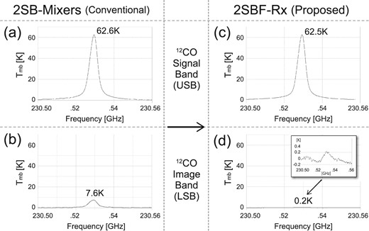
12CO spectra of the observation toward Orion KL using the OPU 1.85 m radio telescope. (a) 12CO spectrum obtained using a conventional receiver system (2SB SIS mixers), and (b) its leakage into the image band. (c) 12CO spectrum obtained using the 2SBF-Rx with the 220/230 GHz FSF, and (d) its leakage into the image band.
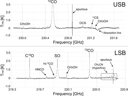
Spectra observed toward Orion KL using the OPU 1.85 m radio telescope for USB and LSB.
We used this 2SBF-Rx for the scientific observations for one winter season, from 2014 December to 2015 May, and no fluctuation of the IRR larger than 1 dB has been observed during the season. These results successfully demonstrated that the proposed 2SBF-Rx works much better than the conventional 2SB SIS mixer receiver when the frequency setting is fixed.
6 Conclusion
A novel sideband separation method was developed for use in heterodyne receivers in the millimeter/submillimeter band using a new waveguide circuit called the FSF, which consists of two quadrature hybrid couplers and two waveguide high-pass filters. This circuit has two main output ports; the USB signal passes through the high-pass filters and to one output port, and the LSB signal is reflected from the filters and passes to another output port. This allows the USB and LSB signals to be separated.
Simulation was performed using the three-dimensional finite element method electromagnetics simulator HFSS, and the optimized S-parameters were obtained for the four ports to realize simultaneous observations of the J = 2–1 rotational transitions of three CO isotopes (12CO, 13CO, and C18O) at 219–230 GHz. A prototype of the FSF was manufactured with a machining error of less than 10 μm, and its measured frequency characteristics were in good agreement with the designed one within the range of machining errors.
Furthermore, a new sideband separation receiver with FSF (2SBF-Rx) was developed and installed in a 1.85 m radio telescope. Observations of molecular clouds revealed that the IRR of the 2SBF-Rx is as high as ∼25 dB for the three CO isotope lines, which is a significant improvement from the IRR of ∼10 dB of the conventional sideband-separating receiver. Moreover, using the 2SBF-Rx has not caused large fluctuations regarding the image rejection performance.
From the above results, the practical applicability of the 2SBF-Rx to radio astronomical observation has been verified successfully verified. The only drawback of this new method is that the observation frequency band is fixed by the internal filters; however, the great advantage is that a very stable IRR and other characteristics can be achieved with only one component. Thus, the proposed method has major advantages in wide frequency band observations with a fixed frequency setting, such as survey-type observations of fixed molecular lines and the monitoring of specific molecules in planetary atmospheres.
Acknowledgements
The authors would like to thank Satoshi Ochiai and Akifumi Kasamatsu of the National Institute of Information and Communications Technology (NICT) and Kenichi Kikuchi of the National Astronomical Observatory of Japan (NAOJ) for measuring the FSF with a VNA at NICT. We are also grateful to Masanori Ishino of Kawashima Manufacturing Co., Ltd. (KMCO) for conducting the high-precision machining of the FSF. We would also like to thank Atsushi Nishimura, Nozomi Okada, Syota Ueda, and all members of the 1.85 m telescope team for installing and operating the developed FSF receiver to verify its performance. And, author would like to appreciate to Dr. Junji Inatani very much for his very kind and careful refereeing.
This work was financially supported by a Japan Society for the Promotion of Science (JSPS) Research Fellowship for Young Scientists DC1 (No. 26-12320), JSPS KAKENHI (Grant Nos. 22244014 and 26247026), and the Toray Science Foundation.
References
