


Abstract
Most relatively warm, unevolved, metal-poor stars (Teff ≳ 5800 K and [Fe/H] ≲ −1.5) exhibit almost constant lithium abundances, irrespective of metallicity or effective temperature, and thus form the so-called Spite plateau. This was originally interpreted as arising from lithium created by the Big Bang nucleosynthesis. Recent observations, however, have revealed that ultra metal-poor stars (UMP stars; [Fe/H] < −4.0) have significantly lower lithium abundances than those of the plateau. Since most of the UMP stars are carbon-enhanced metal-poor stars with no excess of neutron-capture elements (CEMP-no stars), a connection between the carbon enhancement and lithium depletion is suspected. A straightforward approach to this question is to investigate carbon-normal UMP stars. However, only one object is known in this class. As an alternative, we have determined lithium abundances for two CEMP-no main-sequence turn-off stars with metallicities [Fe/H] ∼ −3.0, where there are numerous carbon-normal stars with available lithium abundances that can be considered. Our 1D local thermodynamic equilibrium analysis indicates that the two CEMP-no stars have lithium abundances that are consistent with values near the plateau, which suggests that carbon enhancement and lithium depletion are not directly related. Instead, our results suggest that extremely low iron abundance is a fundamental cause of depleted lithium in UMP stars.
1 Introduction
Very metal-poor stars preserve the chemical composition of their natal gas clouds, hence their elemental abundances have been extensively used to investigate the nature of the first nucleosynthesis processes in the universe (see, e.g., Beers & Christlieb 2005; Frebel & Norris 2015). Lithium is of particular interest, because it is the only “metal” created during the Big Bang. Spite and Spite (1982) first pointed out that metal-poor dwarfs (Teff ≳ 5800 K and [Fe/H] ≲ −1.5)1 have an almost constant lithium abundance, regardless of their effective temperature or metallicity (the so-called “Spite plateau”). The temperature range is limited because lithium abundances dramatically decrease in cooler stars due to deep convection during stellar evolution. In the metallicity range of [Fe/H] > −1.5, production of lithium via, for instance, novae and cosmic ray, can affect the lithium abundances in more metal-rich stars (see Prantzos 2012 for more details). In any event, until relatively recently, the constant value of A(Li) = 2.2 ± 0.1 among unevolved metal-poor stars (e.g., Spite & Spite 1982) was considered likely to represent the primordial lithium abundance emerging from the Big Bang nucleosynthesis.2
Doubts concerning this interpretation emerged when increasingly precise inferences of the expected primordial lithium abundance began to be made, in particular those based on derived estimates of the baryon number density from cosmic microwave background measurements combined with standard Big Bang nucleosynthesis models (Coc et al. 2004; Spergel et al. 2007). In the modern era of precision cosmology, Coc, Uzan, and Vangioni (2014) derived the predicted primordial value of lithium to be A(Li) = 2.66–2.73 based on well-constrained cosmological parameters (Planck Collaboration 2014). This value is higher than the observed value of the lithium abundances for stars on the Spite plateau by ∼0.5 dex.
Following the early studies, observations of metal-poor stars with lower metallicity, which is expected to approach the primordial lithium abundance more closely, have highlighted additional difficulties. Ryan, Norris, and Beers (1999) pointed out that there is a slope to the plateau at [Fe/H] < −2.5 though the star-to-star scatter is very small. They concluded that lithium in metal-poor stars is not primordial but affected by some processes other than the Big Bang, in particular the Galactic chemical evolution. More recent studies have reported the so-called “breakdown” of the Spite plateau at extremely low metallicity, e.g., [Fe/H] ≲ −3, where measured lithium abundances start to exhibit scatter, and extend the mean value to even lower levels (e.g., Aoki et al. 2009; Sbordone et al. 2010). More significantly, no ultra metal-poor (UMP; [Fe/H] < −4) star has been reported to be on the plateau (e.g., Bonifacio et al. 2015). Although the convection mechanisms which can lead to depletion of lithium are expected to be less effective at lower metallicity, some authors have invoked alternative stellar processes capable of depleting lithium that might be active in very metal-poor stars (Meléndez et al. 2010). If such a depletion mechanism inside UMP stars themselves does work, a similar mechanism could bring lithium abundances in less metal-poor stars from A(Li) ≃ 2.7 to the Spite plateau value.
A remarkable feature of UMP stars is the high fraction of carbon-enhanced objects. All carbon-enhanced UMP stars show no excess of heavy neutron-capture elements (Norris et al. 2013b), and are classified into so-called CEMP-no stars (carbon enhanced metal-poor stars without heavy elements enhancement; Beers & Christlieb 2005). For example, HE 1327−2326, which is the most metal-poor main-sequence turn-off star with enhanced carbon abundance, has a very low upper limit on the lithium abundance, A(Li) < 0.70 (Frebel et al. 2005, 2008; Aoki et al. 2006). The fact that most UMP stars are CEMP-no stars leads us to investigate the connection between lithium depletion and carbon excess.
From theoretical viewpoints, a possible relation between carbon enhancement and lithium depletion has been proposed. Piau et al. (2006) suggested that lithium astration in Population III stars, in addition to lithium destruction in stars which are now observed as metal-poor stars, is a possible solution to the lithium problems. The large enhancement of carbon in UMP stars could be attributed to unique yields from Population III stars (e.g., spin star model, Maeder et al. 2015; faint supernovae model, Nomoto et al. 2013, Tominaga et al. 2014). Hence, it is qualitatively possible to assume that UMP stars are formed under the strong influence of Population III stars, which results in carbon enhancement and lithium depletion. Another explanation is that CEMP-no stars underwent mass transfer from a former asymptotic giant branch (AGB) companion in which carbon is enhanced (Suda et al. 2004). The same mechanism is considered to be responsible for the formation of CEMP-s stars (CEMP stars with s-process element enhancement). Since CEMP-s stars are not yet found among UMP stars, CEMP-no stars might be a low metallicity counterpart of CEMP-s stars. Note that reported binary frequency of CEMP-s stars is ∼82% ± 10%, whereas that of CEMP-no stars is 17% ± 9% (Hansen et al. 2016a, 2016b). While lithium might be produced at some phase of AGB evolution through the Cameron–Fowler mechanism (Sackmann & Boothroyd 1992), it is more generally destroyed. In fact, lithium abundance in CEMP-s stars is usually lower depending on the amount of accreted mass (Masseron et al. 2012).
In order to examine the possible connection between lithium depletion and carbon excess at very low metallicity, it is highly desirable to observe carbon-normal stars at [Fe/H] < −4. However, only one unevolved carbon-normal UMP star has been reported (SDSS J102915+172927: Caffau et al. 2012), in spite of recent extensive surveys and their follow-up high-resolution spectroscopic observations (e.g., Aoki et al. 2013; Roederer et al. 2014). Interestingly, this star has very low lithium abundance [A(Li) < 1.1], whereas the upper limit of the carbon abundance is low ([C/Fe] < 0.93).
An alternative approach is to investigate lithium abundances in CEMP-no stars with [Fe/H] ∼ −3 with the assumption that they have the same origin as CEMP-no stars with [Fe/H] < −4. Masseron et al. (2012) reported low lithium abundances in CEMP stars without classifying them into subclasses. However, each subclass of CEMP stars should be discussed separately since they could be formed through different formation processes. The current sample is not large enough to discuss the lithium abundance of CEMP-no stars statistically. Moreover, in order to discuss the relation between lithium and carbon, we need to compare lithium abundances in CEMP-no stars with those of carbon-normal stars with similar metallicity.
In this paper, we determine the lithium abundances in two unevolved CEMP-no stars as well as in comparison stars with normal carbon abundances with [Fe/H] ∼ −3. In section 2, we briefly explain how these objects have been selected and observed. Methods to estimate stellar parameters and to measure abundances are described along with the results in section 3. Finally we give interpretation to them in section 4.
2 Target selection and observation
The sample of the present abundance study includes two CEMP-no stars. One of them, SDSS J1424+5615, is selected from the extremely metal-poor stars studied by Aoki et al. (2013), who derived Teff = 6350 K and [Fe/H] = −2.97 for this object via “snap-shot” spectroscopy. A high-resolution spectrum with R = 60000 covering 4030–6800 Å was obtained with the Subaru telescope's High Dispersion Spectrograph (HDS: Noguchi et al. 2002) on 2009 June 29 (see table 1). Stellar parameters and elemental abundances discussed in this paper are determined from this new spectrum.
Observations of our targets.
| Observation name | RA | Dec | Observation date | Exposure time | S/N | vr |
|---|---|---|---|---|---|---|
| (J2000.0) | (J2000.0) | (min) | (6700 Å) | (km s−1) | ||
| LAMOST J1410−0555 | 14h10m02|${^{s}_{.}}$|83 | −05°55΄51|${^{\prime\prime}_{.}}$|8 | 2014 May 10 | 15 | 113 | 94.89 |
| SDSS J1424+5615 | 14h24m41|${^{s}_{.}}$|88 | +56°15΄35|${^{\prime\prime}_{.}}$|0 | 2009 June 29 | 230 | 95 | −0.13 |
| LAMOST J1305+2815 | 13h05m34|${^{s}_{.}}$|80 | +28°15΄10|${^{\prime\prime}_{.}}$|5 | 2014 May 11 | 15 | 88 | 35.84 |
The other CEMP-no star, LAMOST J1410−0555, is identified in the follow-up high-resolution spectroscopy with the Subaru telescope for candidate metal-poor stars found in the Data Release 1 of LAMOST (the Large sky Area Multi-Object fiber Spectroscopic Telescope; Cui et al. 2012; Luo et al. 2012, 2015; Zhao et al. 2012). A high-resolution spectrum with R = 45000 for 4030–6800 Å was obtained on 2014 May 10. The spectrum of a comparison star, LAMOST J1305+2815, was obtained with the same set-up of HDS (see table 1). See Li et al. (2015a) for more details on the metal-poor star survey with LAMOST and the follow-up study with the Subaru telescope.
Standard data reduction was conducted using the IRAF echelle package, including bias-level correction for the CCD data, scattered light subtraction, flat-fielding, extraction of spectra, and wavelength calibration using Th arc lines.3 The signal-to-noise (S/N) ratios per 1.8 km s−1 pixel are estimated from the standard deviation of photon counts for continuum at 6708 Å (table 1). Heliocentric radial velocities are also provided in table 1. We also analyze the spectrum of G64-12 obtained by Aoki et al. (2006) for comparison purposes. This is a bright, extremely metal-poor ([Fe/H] ≃ −3.3), main-sequence turn-off star that has been the subject of many previous studies (e.g., Stephens & Boesgaard 2002; Barklem et al. 2005; Aoki et al. 2006, 2009; Ishigaki et al. 2010, 2012; Roederer et al. 2014; Placco et al. 2016).
3 Abundance analysis and results
We apply the standard abundance analysis technique using 1D model atmospheres of the ATLAS NEWODF grid assuming no convective overshooting (Castelli & Kurucz 2003). α-enhanced models ([α/Fe] = 0.4) are used since our targets show α element enhancement. Our results are compared with previous ones for a large number of carbon-rich/carbon-normal stars analysed via 1D models. Though a 3D effect is beyond the scope of this paper, it should be noted that Sbordone et al. (2010) and Lind, Asplund, and Barklem (2009a) reported that the 3D and non-local thermodynamic equilibrium (NLTE) correction required for lithium abundances is systematic and not larger than 0.05 dex.
3.1 Stellar parameters
We carried out analysis of Balmer line profiles in order to estimate effective temperature and surface gravity. Model profiles of Balmer lines are computed by Barklem et al. (2002).4 They calculated the profiles with 1D LTE model atmospheres of MARCS of the epoch of 1997 (Asplund et al. 1997, and references therein), using self broadening theory by Barklem, Piskunov, and O’Mara (2000). Assumed parameters of mixing-length theory (MLT) are α = 0.5 and y = 0.5. The grid of the model profiles covers effective temperatures from 4500 K to 7500 K in intervals of 100 K. The surface gravity of the grid spans from 1.0 to 5.0 for Teff ≤ 5500 K and from 3.4 to 5.0 for Teff ≥ 5600 K. For each set of Teff and log g, the metallicity spans from [Fe/H] = −3.0 to [Fe/H] = 1.0, in intervals of 0.5. [α/Fe] = 0.4 models are used during Balmer line analysis.
Normalization of observed spectra around a broad Balmer line is essential to estimate stellar parameters. Following the method described in Barklem et al. (2002), multi-order spectra that do not include Balmer lines are normalized by fitting the continuum level with a spline function, and the continuum profile of the orders including a Balmer line is estimated by the interpolation from adjacent two orders.
We adopt stellar parameters which minimize χ2 as a result of model profile fitting for the shaded regions in figure 1. First, we make an estimation of Teff from the wings of the Hβ line, assuming log g = 4.0 since the shape of the line is sensitive to Teff but not to log g or metallicity. With the estimated Teff, log g is subsequently estimated from the wings of Hα, which depend on both log g and Teff. Then, Teff is redetermined from Hβ with the estimated log g. Finally, log g is redetermined from Hα with the updated Teff. The fitting results of Balmer lines for LAMOST J1410−0555 are shown in figure 1. Metallicity is fixed to [Fe/H] = −3 through Balmer line analysis, though metallicity-dependence on derived parameters is small.
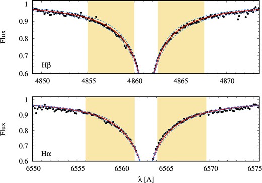
Fitting results for Hβ and Hα of LAMOST J1410−0555. Red solid lines show the best-fitting model spectrum, Teff = 6169 K and log g = 4.21. Blue dashed lines show model spectra with ±0.3 dex offset in log g for Hα, and ±100 K offset in Teff for Hβ. Yellow shaded regions are used in fitting. (Color online)
Stellar parameters obtained for the observed stars together with G64-12 are given in table 2 and plotted in figure 2. All of our program stars are in the main-sequence or subgiant phase, i.e., before the first dredge-up.
![Location of observed stars in the HR diagram. Red dots with two open circles show the two CEMP-no stars of this study. LAMOST J1305+2815 is shown with a blue open circle. Stellar parameters of G64-12 from previous studies are shown with black crosses, and those from our analysis are represented by the open green square. Aoki et al. (2006) adopted Teff = 6390 K for G64-12, though their Balmer line analysis derives Teff = 6300 K. Both of them are shown in the figure and connected to each other by the black solid line. Y2 isochrones (Demarque et al. 2004) assuming [Fe/H] = −3 and T = 10, 12, 14 Gyr are also shown. (Color online)](https://oup.silverchair-cdn.com/oup/backfile/Content_public/Journal/pasj/69/2/10.1093_pasj_psw129/4/m_pasj_69_2_24_f2.jpeg?Expires=1749282835&Signature=XuRZVKJSLxyFxIO99TLDQQoVIJLQCfHprd3WpgtSCGFfvNgiG2CHAXGjRAJ5--fxx63Ln9CdFDl6XVMw~t200-T0KsRWDGLbDQgkbMBUMzzkKJDb13aRIq6Vje4rRUAxvRAvbzhqEWGBPsMcRn9XAJq8k102Em53gjIEboAcJkGrdAqJSz6Z7Nb6PUXSyeALR5u6SDswxmob6rX282XWea2b49y5-Q6airod64zalWnIJzGuAFNOLPs37WiVFW4ovAc8AwbpO-5k7pLCcLE1oc6CHOBV7d0eLVXrrt4rQTUI0jh2uRqG2MOV4eVY5erulu0FWSp4y0NXJ83ClxqLJQ__&Key-Pair-Id=APKAIE5G5CRDK6RD3PGA)
Location of observed stars in the HR diagram. Red dots with two open circles show the two CEMP-no stars of this study. LAMOST J1305+2815 is shown with a blue open circle. Stellar parameters of G64-12 from previous studies are shown with black crosses, and those from our analysis are represented by the open green square. Aoki et al. (2006) adopted Teff = 6390 K for G64-12, though their Balmer line analysis derives Teff = 6300 K. Both of them are shown in the figure and connected to each other by the black solid line. Y2 isochrones (Demarque et al. 2004) assuming [Fe/H] = −3 and T = 10, 12, 14 Gyr are also shown. (Color online)
Parameters and abundances of our targets.*
| LAMOST J1410−0555 | SDSS J1424+5615 | LAMOST J1305+2815 | G64-12 | ||||||||||||||
|---|---|---|---|---|---|---|---|---|---|---|---|---|---|---|---|---|---|
| σ | (N) | Error | σ | (N) | Error | σ | (N) | Error | σ | (N) | Error | ||||||
| T eff | 6169 | 40 | 6088 | 40 | 6102 | 40 | 6291 | 40 | |||||||||
| log g | 4.21 | 0.2 | 4.34 | 0.2 | 3.75 | 0.2 | 4.38 | 0.2 | |||||||||
| v turb | 1.1 | 0.3 | 1.1 | 0.3 | 1.5 | 0.3 | 1.5 | 0.3 | |||||||||
| [Fe/H] | Fe i | −3.19 | 0.11 | 38 | 0.04 | −3.01 | 0.10 | 31 | 0.04 | −2.93 | 0.09 | 51 | 0.04 | −3.36 | 0.05 | 49 | 0.03 |
| A(Li) | Li i | 2.17 | — | s | 0.12 | 2.14 | — | s | 0.11 | 2.10 | — | s | 0.10 | 2.22 | — | s | 0.06 |
| [C/Fe] | CH | 1.53 | — | s | 0.12 | 1.49 | — | s | 0.11 | <1.30 | — | s | 0.11 | <0.93 | — | s | 0.08 |
| [Na/Fe] | Na i | 0.56 | 0.05 | 2 | 0.08 | 0.40 | 0.04 | 2 | 0.08 | −0.07 | 0.06 | 2 | 0.07 | −0.09 | 0.01 | 2 | 0.05 |
| [Mg/Fe] | Mg i | 0.84 | 0.08 | 6 | 0.04 | 0.74 | 0.07 | 6 | 0.04 | 0.30 | 0.08 | 7 | 0.04 | 0.36 | 0.04 | 5 | 0.03 |
| [Ca/Fe] | Ca i | 0.34 | 0.09 | 10 | 0.03 | 0.16 | 0.17 | 6 | 0.07 | 0.43 | 0.08 | 16 | 0.02 | 0.51 | 0.06 | 18 | 0.02 |
| [Sc/Fe] | Sc ii | 0.26 | 0.07 | 2 | 0.10 | 0.35 | 0.09 | 2 | 0.10 | 0.34 | 0.03 | 7 | 0.07 | 0.28 | 0.12 | 4 | 0.09 |
| [Ti/Fe] | Ti i | 0.52 | 0.06 | 3 | 0.06 | 0.83 | 0.00 | 1 | 0.10 | 0.64 | 0.11 | 5 | 0.05 | 0.66 | 0.09 | 6 | 0.04 |
| [Ti/Fe] | Ti ii | 0.23 | 0.06 | 10 | 0.07 | 0.28 | 0.07 | 9 | 0.07 | 0.48 | 0.10 | 17 | 0.07 | 0.57 | 0.05 | 18 | 0.07 |
| [Cr/Fe] | Cr i | −0.32 | 0.05 | 5 | 0.02 | −0.30 | 0.11 | 4 | 0.06 | −0.22 | 0.04 | 5 | 0.02 | −0.11 | 0.02 | 4 | 0.01 |
| [Fe/Fe] | Fe ii | −0.03 | 0.12 | 6 | 0.09 | 0.11 | 0.08 | 6 | 0.08 | −0.04 | 0.11 | 11 | 0.08 | 0.11 | 0.07 | 12 | 0.08 |
| [Sr/Fe] | Sr ii | −0.10 | 0.00 | 1 | 0.12 | −0.40 | 0.00 | 1 | 0.11 | 0.28 | 0.00 | 1 | 0.10 | — | 0 | — | |
| [Ba/Fe] | Ba ii | −0.33 | 0.00 | 2 | 0.10 | <−0.69 | — | — | — | −0.38 | 0.05 | 3 | 0.09 | −0.08 | 0.02 | 2 | 0.08 |
*Fe in [X/Fe] denotes iron abundance from Fe i lines. Solar abundances are from Asplund et al. (2009). Total error for each abundance includes σ2/N and those due to internal error in stellar parameters.
In most cases, Teff and log g from Balmer lines yield consistent results with the ionization and excitation balance of iron. vturb is determined as not producing a trend in iron abundance with equivalent width (see table 2). The uncertainty of vturb is determined so that the trend does not become significant at 1σ level.
Uncertainties in Teff and log g due to Poisson noise are estimated using a Monte Carlo method. 100 spectra are generated by adding noise to a synthetic spectrum calculated by the model atmosphere of Teff = 6200 K, log g = 4.2, and [Fe/H] = −3.0, assuming the noise has a Gaussian distribution of which the standard deviation is (S/N)−1. Teff and log g are re-determined for these spectra with the above procedure of profile-fitting for Balmer lines. We take the standard deviation of the results obtained for the 100 spectra as the uncertainty. The resultant uncertainty is ∼5 K in Teff and ∼0.02 dex in log g for a spectrum with S/N ∼ 100, indicating that the uncertainty due to random noise of spectra is sufficiently small. On the other hand, the uncertainty of the continuum level has a larger impact on the stellar parameters. The accuracy of interpolation in the normalization procedure is estimated to be 0.5% by comparing continuum spectra from interpolation with those from the direct normalization technique for orders that are free from broad absorption lines. We assume that the accuracy of interpolation does not significantly depend on S/N for spectra with S/N > 50 and with [Fe/H] < −3, where the number of absorption lines is small. A 0.5% change in continuum level leads to ΔTeff ∼ 35 K and Δlog g ∼ 0.15 dex. Therefore, we take ΔTeff ∼ 40 K and Δlog g ∼ 0.2 dex as total uncertainty for stellar parameters.
In addition to these random errors, systematic errors due to the uncertainty of the model profile calculations should exist. A possible estimation of the systematic errors is to compare the stellar parameters with values obtained by other methods. Norris et al. (2013a) determined effective temperature and surface gravity for metal-poor stars through three different procedures: spectrophotometry, Balmer line profile fitting, and the Hδ index HP2. They reported a systematically lower effective temperature from Balmer lines than that from spectrophotometry by 128 K in average. We note that Balmer line profiles computed from 3D hydrodynamical calculation of stellar atmosphere are sharper than those from 1D calculation, assuming α = 0.5, which leads to hotter Teff in 3D Balmer line analysis (Ludwig et al. 2009). Adopting a temperature lower by 128 K at Teff ∼ 6200 K leads to 0.10 dex lower [Fe/H], 0.09 dex lower A(Li), 0.12 dex lower [C/Fe], and 0.02 dex higher [Ba/Fe].
Very recently, the data release 1 of the Gaia satellite (Gaia Collaboration 2016) became available. The data release contains parallaxes of LAMOST J1410−0555, LAMOST 1305+2815, and G64-12. We derive log g for them from their parallaxes and photometric data (APASS DR9 for LAMOST J1410−0555 and G64-12, Henden et al. 2016; SDSS DR10 for LAMOST J1305+2815, Ahn et al. 2014). Computed log g is 4.3 ± 0.1 for LAMOST J1410−0555, 4.3 ± 0.1 for G64-12, and |$3.9^{+0.3}_{-0.7}$| for LAMOST J1305+2815. Our log g values from Hα lines are in fairly good agreement with those derived from the Gaia parallaxes.
We here compare the stellar parameters of some individual stars with those from previous studies. Stellar parameters of G64-12 from various studies are listed in table 3. Our Teff estimation is consistent with previous ones obtained via Balmer line analysis, whereas Teff from the excitation equilibrium of iron is systematically lower (Stephens & Boesgaard 2002; Ishigaki et al. 2010; Roederer et al. 2014). A similar trend has been reported for very metal-poor giants by Frebel et al. (2013). The three studies that derived lower surface gravity (log g < 4) are based on the excitation equilibrium of iron to derive the effective temperature (table 3). The discrepancy in log g between our study and that of Stephens and Boesgaard (2002) or Ishigaki et al. (2010) is partly due to lower effective temperature. They determined log g by requiring an ionization equilibrium. In order to compensate neutralization by lower Teff, log g has to be lowered by ∼0.2 dex per 100 K. In addition, the NLTE effect should cause overionization, and affect the iron abundance derived from Fe i lines whereas that from Fe ii lines is not changed (e.g., Thévenin & Idiart 1999). Therefore, lower log g is needed to achieve ionization equilibrium in 1D LTE analysis since it derives higher iron abundance from Fe ii lines than that from Fe i lines. Likely these two processes cause the discrepancy. On the other hand, a lower log g is obtained by Roederer et al. (2014) assuming its evolutionary phase from the isochrones of a subgiant. We note that the Gaia parallax indicates that G64-12 is in the main-sequence phase.
Comparison of stellar parameters and abundances of G64-12.
| This work | Previous studies * | |||||||||
|---|---|---|---|---|---|---|---|---|---|---|
| (1) | (2) | (3) | (4) | (5) | (6) | (7) | (8) | |||
| T eff † | 6291 | 6270 | 6390 | 6141 | 6550 | 6074 | 6463 | 6070 | 6030 | |
| B | B | Hd & C‡ | C | C | E | IRFM | E | E | ||
| log g† | 4.38 | 4.4 | 4.38 | 4.25 | 4.68 | 3.72 | 4.26 | 3.58 | 3.6 | |
| B | Ic | Ic | I | I | I§ | P | I | Ic | ||
| v turb | 1.5 | 1.5 | 1.6 | 1.49 | 1.9 | 1.19 | 1.65 | 1.46 | 1.2 | |
| [Fe/H] | Fe i | −3.36 | −3.37 | −3.2 | −3.44 | −3.24 | −3.47 | −3.29 | −3.56 | −3.58 |
| A(Li) | Li i | 2.22 | 2.18 | 2.3 | 2.36 | 2.08 | ||||
| [C/Fe] | CH | <0.93 | 0.49 | 0.71 | 1.07 | <0.91 | ||||
| [Na/Fe] | Na i | −0.09 | −0.06 | −1.13 | −0.09 | −0.06 | ||||
| [Mg/Fe] | Mg i | 0.36 | 0.37 | 0.46 | 0.55 | 0.32 | 0.63 | 0.48 | 0.76 | 0.50 |
| [Ca/Fe] | Ca i | 0.51 | 0.46 | 0.48 | 0.56 | 0.61 | 0.50 | 0.51 | 0.62 | |
| [Sc/Fe] | Sc ii | 0.23 | 0.17 | −0.24 | ||||||
| [Ti/Fe] | Ti i | 0.66 | 0.53 | 0.74 | 0.70 | |||||
| [Ti/Fe] | Ti ii | 0.57 | 0.38 | 0.64 | 0.47 | 0.52 | 0.60 | 0.11 | ||
| [Cr/Fe] | Cr i | −0.11 | −0.18 | −0.10 | 0.07 | −0.09 | −0.10 | −0.20 | ||
| [Fe/Fe] | Fe ii | 0.11 | 0.13 | −0.02 | 0.07 | 0.05 | 0.00 | 0.19 | ||
| [Sr/Fe] | Sr ii | 0.08 | 0.18 | 0.06 | 0.18 | 0.07 | −0.10 | |||
| [Ba/Fe] | Ba ii | −0.08 | −0.25 | 0.07 | 0.06 | −0.2 | −0.07 | −0.25 | −0.46 | |
*(1): Aoki et al. (2009), (2): Aoki et al. (2006), (3): Barklem et al. (2005), (4): Ishigaki et al. (2012), (5): Stephens and Boesgaard (2002), (6): Placco et al. (2016), (7): Ishigaki et al. (2010), (8): Roederer et al. (2014).
†The methods used to determine Teff and log g are shown. B: Balmer line analysis, Hd: Hδ index, C: color, E: excitation equilibrium of Fe i, IRFM: Infrared flux method, Ic: isochrones, I: ionization equilibrium of Fe i and Fe ii, P: photometric indices.
‡Aoki et al. (2006) determines Teff from several methods. Although their Balmer line analysis yields Teff = 6300 K, they adopt the average of Teff from colors and from the Hδ index.
§log g by Stephens & Boesgaard 2002 is the averaged value of one which achieve ionization equilibrium of iron and one which achieve that of titanium.
Aoki et al. (2013) derived Teff of SDSS J1424+5615 as 5971 K from its (V − K) color and 6266 K from its (g − r) color, but adopted 6339 K based on the estimate made by the SDSS SEGUE pipeline (SSPP) of DR7 (Abazajian et al. 2009). The updated version of the SSPP of DR8 (Lee et al. 2008) provides Teff = 6402 K. Our derived Teff of 6088 K is slightly lower than the value of Aoki et al. (2013), but is within the uncertainty of these estimates.
3.2 Abundance analysis
We apply standard analysis to equivalent widths measured for clean lines that are apparently not affected by blending after each line is fitted with a Gaussian profile. The line list is taken from Aoki et al. (2013) except for the CH G-band and Li i doublet. The effect of hyperfine splitting of Ba ii and Sc ii are included following McWilliam (1998) and McWilliam et al. (1995), respectively. The uncertainty of determined abundance is estimated as |$\sqrt{\sigma ^2/N}$|, where σ is the standard deviation of abundances determined from individual lines, and N is the number of lines measured for the element. For elements with fewer than three measurable absorption lines, the uncertainty of the abundance measurement is estimated by adopting the σ value of Fe abundances from Fe i lines in the above formula. We also include errors that come from uncertainty in stellar parameters. The errors are estimated by measuring abundances using a model atmosphere with the offset in stellar parameters, corresponding to the uncertainty in derived stellar parameters.
The abundances of carbon and lithium are determined by fitting observed spectra with synthetic spectra. The carbon abundance is determined from the CH G-band around 4324 Å and the lithium abundance is from the doublet around 6708 Å. Synthetic spectra are convolved with an instrumental profile, a rotational profile and/or macroturbulance using a Gaussian profile, of which the FWHM is estimated from iron lines. The line list of the CH G-band is taken from Masseron et al. (2014), and that of Li i doublet is from the line list of 7Li in Smith et al. (1998). Sometimes observed spectrum is shifted vertically to derive appropriate continuum level and horizontally to match the line center. The abundance is determined as the value which gives the minimal χ2. We confirm that the best-fitting synthesized spectra well reproduce the observed one, in order to exclude incorrect fitting due to bad columns and/or cosmic rays. The error in fitting estimated with a Monte Carlo method is ∼0.02 dex, which is much smaller than the σ of Fe i lines. We adopt the σ value of Fe lines as the uncertainty of abundances of carbon and lithium in order to take into account other sources of error, such as uncertainty in oscillator strength or normalization. We also include errors that stem from uncertainties in stellar parameters which are estimated in the same way as for the other elements.
Results of the abundance analysis are given in table 2. Internal errors are included, but systematic errors due to determination methods of stellar parameters are not.
We compare derived abundances of G64-12 with previous studies in table 3. In particular, the abundances of [Fe/H], A(Li), and [Ba/Fe] of our study are consistent with previous studies which derived similar stellar parameters. We note that, although Placco et al. (2016) have determined the carbon abundance of G64-12, the strongest part of the CH G-band of our spectra unfortunately hits bad columns. The difference between the carbon abundance measured by Placco et al. (2016) and our upper limit is likely due to the different choice of effective temperature.
Fitting results for CH G-band of LAMOST J1410−0555 and SDSS J1424+5615 are shown in figure 3. For SDSS J1424+5615, there are no detectable Ba ii lines in its spectrum. Figure 4 shows the spectrum around the strongest Ba ii line and the model spectrum assuming [Ba/Fe] = −0.67. We have also examined the presence of a Eu ii line at ∼4129 Å, but do not find any absorption feature at this wavelength ([Eu/Fe] < +2.0). Since both stars have [C/Fe] > 1.0 and [Ba/Fe] < 0, they are unquestionably CEMP-no stars.
![Fitting results for CH G-bands around 4322 Å. The spectrum of SDSS J1424+5615 is shifted vertically. The red solid lines show the best-fitting spectra and the blue dashed ones show the spectra with an offset of ±0.2 dex in [C/Fe]. (Color online)](https://oup.silverchair-cdn.com/oup/backfile/Content_public/Journal/pasj/69/2/10.1093_pasj_psw129/4/m_pasj_69_2_24_f3.jpeg?Expires=1749282835&Signature=hFAWsSnLjrktxW58Pj1gIURjrFPyC4OKqpDrZoHFBMQyWkTiAEkPy-KTkVyVx5NpvEtrmqjXxRCFQ8X7-TgY2N86dzpIAPVKweCawcP7iYKQKCQnTvXat~cIaxyfHua0SIjDn3UntiSfg1DFubfK30jmnbu726QOeZfaXNFa5StVOjngBIHBF3gAFZlToGKeKcbjcAKWRHv252lEIyfn4B2ROkPiXSnrKG0yMGMLmNJ6uN~VmYUqcxuFoBqpqZhLQy-dJN8iPMuefgCNod168x6rAXxpt8gBz76hKBmeQEMu6jvJkRwFQDCxWOqcKBWB7Xb3i-YqV3q5SGvm2voo5w__&Key-Pair-Id=APKAIE5G5CRDK6RD3PGA)
Fitting results for CH G-bands around 4322 Å. The spectrum of SDSS J1424+5615 is shifted vertically. The red solid lines show the best-fitting spectra and the blue dashed ones show the spectra with an offset of ±0.2 dex in [C/Fe]. (Color online)
![Comparison of a model spectrum ([Ba/Fe] = −0.67) and SDSS J1424+5615 spectrum for Ba ii 4554 Å. This results in the upper Ba abundance limit of [Ba/Fe] < −0.67 for this object. (Color online)](https://oup.silverchair-cdn.com/oup/backfile/Content_public/Journal/pasj/69/2/10.1093_pasj_psw129/4/m_pasj_69_2_24_f4.jpeg?Expires=1749282835&Signature=u7qdLguptbhgwm8xBESWaxd37Ww6vx38zJsFGmAqT~ACmsPBZtMPPm5IkVNxIiijVc7KjLQ6FJ3eLXE84Sc6airQONYU8WuS7T8CrKrzW9Pr7lFca7BEs2UMYwHbQBYxim2I1w~FCqeaSHKPSGpu91LDXycahWt-gXqafGMle~EwORPa-NaDFo-FOZvszSH72BCJ2i51X-OHozLjFXxoDnONyd1D5bGzI5cg0vq2oQH4Cfp3Oo5zMqQaQknCC3BugfhaGZXzllz~RtuxlcoT2yyM0D2UQ7eYvbJjxZhOjSZ2Y~qTn-RUmlTE06NMkedVzO2sJBx5-w7dsWTsKkIBfQ__&Key-Pair-Id=APKAIE5G5CRDK6RD3PGA)
Comparison of a model spectrum ([Ba/Fe] = −0.67) and SDSS J1424+5615 spectrum for Ba ii 4554 Å. This results in the upper Ba abundance limit of [Ba/Fe] < −0.67 for this object. (Color online)
Fitting results for the Li i doublet of LAMOST J1410−0555 and SDSS J1424+5615 are presented in figure 5. The lithium abundance of both stars is A(Li) ∼ 2.15 dex, placing them on the Spite plateau.
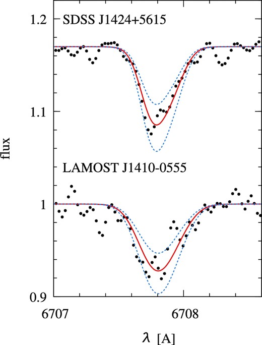
Same as figure 3 but for Li i 6708 Å. (Color online)
It should be noted that both of the CEMP-no stars show large enhancement in magnesium abundance, while other α elements show no excess. Sodium is also enhanced in these stars. Although these abundance anomalies may be a clue to the understanding of CEMP-no stars, it is beyond the scope of this paper.
4 Discussion
4.1 Data compilation
Figure 6 shows lithium abundances as a function of [Fe/H] for our targets together with the data taken from the SAGA database (Suda et al. 2008, 2011; Yamada et al. 2013). The database compiles abundances of halo stars from various literature. It sometimes contains multiple measurements for one star if more than one paper provided an abundance. The following criteria are those we adopt to select main-sequence turn-off metal-poor stars and to classify stars into subclasses.
Main-sequence turn-off metal-poor stars: all measurements by different studies give (i) Teff ≥ 5800 K, (ii) log g ≥ 3.7, and (iii) [Fe/H] ≤ −1.5.
![A(Li) as a function of [Fe/H]. Black dots show carbon-normal stars, grey dots are stars without carbon measurement and CEMP candidates, green squares are CEMP-s stars, red dots with a circle are CEMP-no stars, and yellow crosses are CEMP stars that cannot be classified. Our new CEMP-no stars are red dots with double circles. The Spite plateau (A(Li) = 2.2 ± 0.1; [Fe/H] > −2.5) is indicated by the yellow region. Note that the lithium abundance of CEMP-no stars is comparable to that of carbon-normal stars at −3.5 < [Fe/H] < −2.0 (the blue shaded region), whereas that of CEMP-s stars is lower. (Color online)](https://oup.silverchair-cdn.com/oup/backfile/Content_public/Journal/pasj/69/2/10.1093_pasj_psw129/4/m_pasj_69_2_24_f6.jpeg?Expires=1749282835&Signature=qmDkiru4D3y1d-KjDsjf7f6Acxu0aNdqiY8ilLYbnREFfYimkyFoLfjfLWA2Md4~JZnu4WjzimNpT3HUVntcJ3pyMhqYHYbf3HRxlISYwLy~dpklJ8e9O~p-rw2ojxwsucijxJEMV0hDqJZM-DVw-arbGdCvtPLyijU8~4Ja2Ff8gnCx0GxTukkojAEYz59f3iyiuXb9U7gnt-8L9k8~MMUZrDw6ngSHobWtj-kLIspG2u~1N43rTOUta~hPxmeaP8KZLTJF89oJAdD9nw5bdaFqEN60~OgAzl6ul~yPP7rxdeD-oj5HmFEpulKFBfkEsD-TdElBZsU4mS8rbGjMaA__&Key-Pair-Id=APKAIE5G5CRDK6RD3PGA) Fig. 6.
Fig. 6.A(Li) as a function of [Fe/H]. Black dots show carbon-normal stars, grey dots are stars without carbon measurement and CEMP candidates, green squares are CEMP-s stars, red dots with a circle are CEMP-no stars, and yellow crosses are CEMP stars that cannot be classified. Our new CEMP-no stars are red dots with double circles. The Spite plateau (A(Li) = 2.2 ± 0.1; [Fe/H] > −2.5) is indicated by the yellow region. Note that the lithium abundance of CEMP-no stars is comparable to that of carbon-normal stars at −3.5 < [Fe/H] < −2.0 (the blue shaded region), whereas that of CEMP-s stars is lower. (Color online)
C-normal/CEMP stars: All measurements give [C/Fe] below/above 0.7. When at least one of the measurements gives [C/Fe] > 0.7 and the others give [C/Fe] < 0.7 for the same star, it is classified as a “CEMP candidate”.
CEMP-no/CEMP-s stars: a simple cut in [Ba/Fe] is traditionally used to classify CEMP stars. Most UMP stars, however, do not have tight enough upper limit on [Ba/Fe] to classify them into CEMP-no stars because of their very low iron abundances. Taking into consideration the increasing trend in [Ba/Fe] with [C/Fe] among CEMP-s stars (see, e.g., Aoki et al. 2007), we introduce new criteria for CEMP-s/CEMP-no stars: for [C/Fe] < 2, objects with [Ba/Fe] > 1 are classified into CEMP-s and those with [Ba/Fe] < 0 are CEMP-no stars. For [C/Fe] > 2, [Ba/C] > −1 and [Ba/C] < −2 are adopted as criteria for CEMP-s and CEMP-no stars, respectively (see figure 7). Eu abundance is not used to classify CEMP stars, thus CEMP-s stars could contain some CEMP-r/s stars. In the case that no measurement of barium abundance is available, or its barium abundance falls between the borders, the star is dealt with as an “unclassifiable CEMP star” in this paper.
![[Ba/C] as a function of [C/Fe]. Two solid lines show the criteria used in this study to classify CEMP stars into subclasses. Our two new stars meet the criteria of CEMP-no stars (red dots with two circles). (Color online)](https://oup.silverchair-cdn.com/oup/backfile/Content_public/Journal/pasj/69/2/10.1093_pasj_psw129/4/m_pasj_69_2_24_f7.jpeg?Expires=1749282835&Signature=z-1wL2mDkJNyBmO9jljpHWoNpu68MqTS15Xs6H9N~oQ2KO8OaZ4aAmFfoT6D~U7-NXnRvrAAknedSWvSWu9Eq7GLlf6I5FgVjKgFxEjbGHtAHioyxUFxhBuLfHZRE1RneYD56eTTR0HheuwRVPq2dBjs2E4pL3QA6ujeN14oSoUk41YuX4NbX~VKwEu2VqJR-060NvRC0PqeRo1I3KSWXQGOByGUndRsHd-iIeAgWUwtN8TokjvUq20yNsVR6zqpY0U1Tc~I6PF1mUNiwOE1KsL5NyRvciFARA7QW8rozCCJshB6Lk1CJO~wHnu9m2gBAZE3y6khRnIjqddMVAvWig__&Key-Pair-Id=APKAIE5G5CRDK6RD3PGA) Fig. 7.
Fig. 7.[Ba/C] as a function of [C/Fe]. Two solid lines show the criteria used in this study to classify CEMP stars into subclasses. Our two new stars meet the criteria of CEMP-no stars (red dots with two circles). (Color online)
If a CEMP star has multiple measurements, we select one of them (the first reference for each star in table 4) as the abundance of the star to plot in figures 6, 7, and 8. For carbon-normal stars and CEMP candidates, we simply adopt the average of multiple measurements in our discussion.
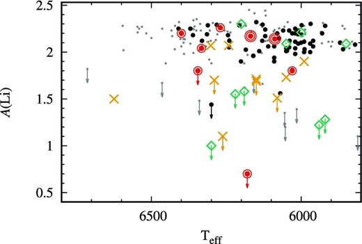
A(Li) as a function of Teff. Symbols are the same as figure 6. (Color online)
Abundances of CEMP stars.
| Object | T eff | log g | [Fe/H] | A(Li) | [C/Fe] | [Ba/Fe] | A(C)† | Reference |
|---|---|---|---|---|---|---|---|---|
| CEMP-no stars | ||||||||
| LAMOST J1410−0555 | 6169 | 4.21 | −3.19 | 2.17 | 1.53 | −0.33 | 6.77 | this work |
| SDSS J1424+5615 | 6088 | 4.34 | −3.01 | 2.14 | 1.49 | <−0.69 | 6.91 | this work |
| CS 29493−050 | 6270 | 3.8 | −2.89 | 2.26 | 0.81 | −0.72 | 6.35 | 1 |
| CS 29514−007 | 6400 | 3.85 | −2.81 | 2.2 | 0.88 | −0.16 | 6.50 | 1 |
| 6281 | 4.1 | −2.8 | 2.24 | 2 | ||||
| HE 1327−2326 | 6180 | 3.7 | −5.71 | <0.70 | 4.06 | <1.24 | 6.78 | 3 |
| 6180 | 3.7 | −5.66 | <1.5 | 4.26 | <1.46 | 7.03 | 4 | |
| 6180 | 3.7 | −5.7 | 4.0 | 5 | ||||
| LAMOST J1253+0753 | 6030 | 3.7 | −4.02 | 1.80 | 1.59 | <−0.30 | 6.00 | 6 |
| SDSS J0212+0137 | 6333 | 4.0 | −3.57 | 2.04 | 2.21 | 0.02 | 7.07 | 7 |
| CEMP-s stars | ||||||||
| CS 22879−029 | 5920 | 3.7 | −2.55 | <1.28 | 1.26 | 1.18 | 7.10 | 1 |
| 6300 | 3.90 | −1.93 | 1.30 | 7.80 | 8 | |||
| CS 22881−036 | 5940 | 3.7 | −2.34 | <1.22 | 1.99 | 2.03 | 8.08 | 1 |
| 6200 | 4.0 | −2.05 | 1.96 | 1.93 | 8.34 | 9 | ||
| CS 22896−136 | 6190 | 3.85 | −2.41 | <1.58 | 1.08 | 1.22 | 7.10 | 1 |
| CS 22956−102 | 6220 | 3.85 | −2.39 | <1.55 | 2.03 | 1.81 | 8.07 | 1 |
| CS 22949−008a | 6300 | 4.0 | −2.14 | <1.0 | 1.44 | 1.41 | 7.73 | 10 |
| CS 22964−161A | 6050 | 3.7 | −2.39 | 2.09 | 1.35 | 1.45 | 7.39 | 11 |
| CS 22964−161B | 5850 | 4.1 | −2.41 | 2.09 | 1.15 | 1.37 | 7.17 | 11 |
| CS 31062−012 | 6200 | 4.3 | −2.53 | 2.3 | 2.14 | 2.08 | 8.04 | 12 |
| 6250 | 4.5 | −2.55 | 2.1 | 1.98 | 7.98 | 13 | ||
| 6000 | 3.8 | −2.74 | 2.15 | 2.01 | 7.94 | 14 | ||
| 5901 | 4.5 | −3.50 | 1.973 | 15 | ||||
| SDSS J1036+1212 | 6000 | 4.0 | −3.2 | 2.21 | 1.47 | 1.17 | 6.70 | 16 |
| 5850 | 4.0 | −3.47 | 1.84 | 1.35 | 6.80 | 17 | ||
| Unclassifiable CEMP stars | ||||||||
| CS 22882−012 | 6290 | 3.8 | −2.76 | <1.7 | 1.09 | 0.61 | 6.76 | 1 |
| CS 22945−017 | 6080 | 3.7 | −2.89 | <1.51 | 1.78 | 0.49 | 7.32 | 1 |
| CS 29504−006 | 6150 | 3.7 | −3.12 | <1.69 | 1.39 | 0.21 | 6.70 | 1 |
| SDSS J1742+2531 | 6345 | 4.0 | −4.80 | <1.80 | 3.63 | <1.72 | 7.26 | 7 |
| SDSS J1035+0641 | 6262 | 4.0 | <−5.05 | <1.1 | 3.08 | <2.25 | 6.70 | 7 |
| CS 29527−015 | 6242 | 4.00 | −3.44 | 2.07 | 18 | |||
| 6242 | 4.00 | −3.55 | 1.18 | 6.06 | 19 | |||
| CS 29528−041 | 6150 | 4.00 | −3.3 | 1.71 | 1.59 | 0.97 | 6.72 | 20 |
| CS 31080−095 | 6050 | 4.50 | −2.85 | 1.73 | 2.69 | 0.77 | 8.27 | 20 |
| HE 0024−2523 | 6625 | 4.3 | −2.72 | 1.5 | 2.6 | 1.46 | 8.31 | 21 |
| HE 1148−0037 | 5990 | 3.7 | −3.46 | 1.90 | 22 | |||
| 5964 | 4.16 | −3.47 | 0.84 | 5.80 | 23 | |||
| HE 1413−1954 | 6302 | 3.80 | −3.50 | 2.04 | 2 | |||
| 6533 | 4.59 | −3.19 | 1.45 | 6.69 | 23 | |||
| CEMP candidates | ||||||||
| CS 22953−037 | 6364 | 4.25 | −2.89 | 2.16 | 0.37 | 5.91 | 19 | |
| 6150 | 3.7 | −3.21 | 1.97 | 0.84 | <−0.67 | 6.06 | 1 | |
| CS 22964−214 | 6800 | 4.5 | −2.30 | 1.0 | −0.12 | 7.13 | 24 | |
| 6180 | 3.75 | −2.95 | 2.02 | 0.62 | −0.54 | 6.10 | 1 | |
| CS 22965−054 | 6205 | 3.73 | −3.09 | <1.07 | <−0.48 | 25 | ||
| 6310 | 3.9 | −2.84 | 2.16 | 22 | ||||
| 6089 | 3.75 | −3.04 | 0.62 | 6.01 | 19 | |||
| 6050 | 3.7 | −3.17 | 2.16 | 0.74 | <−0.45 | 6.00 | 1 | |
| G64-12 | 6462 | 4.26 | −3.29 | 2.36 | 1.07 | −0.07 | 6.21 | 26 |
| G64-37 | 6570 | 4.40 | −3.11 | 2.25 | 1.12 | −0.36 | 6.44 | 26 |
| 6318 | 4.16 | −3.12 | 0.29 | 5.72 | 27 | |||
| 6396 | 3.85 | −2.96 | 2.08 | 15 | ||||
*The first reference for each star in this table is adopted in this study. Where the first reference does not provide some of the parameters, the second one is referred to for those parameters.
† A(C) is converted using the solar abundance of Asplund et al. (2009), while other values are taken directly from the SAGA database, i.e., there remains a solar abundance difference.
‡References. 1: Roederer et al. (2014), 2: Sbordone et al. (2010), 3: Frebel et al. (2008), 4: Aoki et al. (2006), 5: Frebel et al. (2006), 6: Li et al. (2015a), 7: Bonifacio et al. (2015), 8: Johnson et al. (2007), 9: Preston and Sneden (2001), 10: Masseron et al. (2012), 11: Thompson et al. (2008), 12: Aoki et al. (2008), 13: Aoki et al. (2002), 14: Norris et al. (1997), 15: Charbonnel and Primas (2005), 16: Behara et al. (2010), 17: Aoki et al. (2013), 18: Bonifacio et al. (2007), 19: Bonifacio et al. (2009), 20: Sivarani et al. (2006), 21: Lucatello et al. (2003), 22: Aoki et al. (2009), 23: Barklem et al. (2005), 24: Sneden et al. (2003), 25: Lai et al. (2008), 26: Placco et al. (2016), 27: Akerman et al. (2004).
§See table 3 for the results from other studies.
Our new criteria make it possible to classify UMP stars based on their current upper limits on barium abundances. In our literature sample, our new criteria enables us to classify HE 1327−2326 ([C/Fe] = 4.06 and [Ba/Fe] < 1.24; Frebel et al. 2008) as a CEMP-no star.
In addition, an EMP star, SDSS J0212+0137 (Bonifacio et al. 2015), is classified as a CEMP-no star, though its barium abundance ([Ba/Fe] = +0.02) is slightly higher than the traditional criteria of CEMP-no stars. It should be noted that, though one star in the literature sample, HE 0024 −2523 ([Fe/H] = −2.72; Lucatello et al. 2003), was classified as a CEMP-s star with the traditional criteria, it cannot be classified as a CEMP-s nor as a CEMP-no star with the new criteria.
Recently, Yoon et al. (2016) argued that CEMP stars should be classified according to A(C), with A(C) > 7.1 as CEMP-s and A(C) ≤ 7.1 as CEMP-no stars. Although most of the CEMP-no and CEMP-s stars in table 4 are not affected by the choice of classification, we also examine the lithium abundances for the various stellar sub-classes using this criteria.
4.2 Lithium abundances for CEMP subclasses
Since the purpose of this paper is to examine lithium abundance in CEMP-no stars with [Fe/H] ∼ −3, the following discussion is focused on stars within the metallicity range of −3.5 < [Fe/H] < −2.0 (blue-shaded region in figure 6).
By taking a glance at the figure, the plateau of the lithium abundance can be easily found for carbon-normal stars, though some scatter exists, in particular, at [Fe/H] ≲ −3. Most stars without carbon excess marked with black points in the figure have lithium abundance between A(Li) = 1.8 and A(Li) = 2.4. Thus, we define stars with 1.8 < A(Li) < 2.4 as lithium-normal and those with A(Li) < 1.8 as lithium-depleted. No objects with A(Li) > 2.4 is found in the present sample. Based on the criteria, only two out of the 63 carbon-normal stars are classified as lithium-depleted stars (table 5). One is HE 0411−3558 (Teff = 6300 K, log g = 3.7, [Fe/H] = −2.8, [C/Fe] < 0.7, and A(Li) < 1.44; Hansen et al. 2015) and the other is CS 22957-019 (Teff = 6070 K, log g = 3.75, [Fe/H] = −2.43, [C/Fe] = 0.34, and A(Li) = 1.56; Roederer et al. 2014). Ryan et al. (2002) investigated lithium-depleted stars at higher metallicity ([Fe/H] ∼ −1.5) and concluded that the low lithium abundances could be the result of mass transfer. Although HE 0411−3558 and CS 22957-019 show no radial velocity variation as a result of multiple observations, the radial velocity monitoring could be insufficient or the system could be face-on. However, no significant abundance anomalies that could be considered as a result of mass transfer are found within the measurement errors (Hansen et al. 2015; Roederer et al. 2014).
Lithium-depleted fraction for each subclass.
| C-normal | CEMP-s | CEMP-no | |
|---|---|---|---|
| Li-normal (1.8 < A(Li) < 2.4) | 61 | 4 | 4 |
| Li-depleted (A(Li) < 1.8) | 2 | 5 | 0 |
| Li-depleted fraction | 0.032 | 0.556 | 0.000 |
| C-normal | CEMP-s | CEMP-no | |
|---|---|---|---|
| Li-normal (1.8 < A(Li) < 2.4) | 61 | 4 | 4 |
| Li-depleted (A(Li) < 1.8) | 2 | 5 | 0 |
| Li-depleted fraction | 0.032 | 0.556 | 0.000 |
On the other hand, five of the nine CEMP-s stars are lithium-depleted (green open squares, figure 6; see also table 5). This can be interpreted as a result of mass transfer from former AGB companions which should have become white dwarfs, as discussed in section 1. The other four CEMP-s stars are lithium-normal, this could be the result of small amounts of transferred mass which would lead to carbon- and barium-excesses without severe lithium depletion (Masseron et al. 2012; but see also Stancliffe 2010).
It has been difficult to form any discussion on lithium abundance in CEMP-no stars at [Fe/H] ∼ −3 because of the small sample size. We add two CEMP-no stars with lithium measurements to the sample. Together with CS 29493-050 and CS 29514-007 from Roederer et al. (2014), it now becomes possible to discuss the lithium abundance in CEMP-no stars for the first time. The four CEMP-no stars with measured lithium abundance in the metallicity range, −3.5 < [Fe/H] < −2.0, are lithium-normal (table 5). Furthermore, the two CEMP-no stars at lower metallicity, SDSS J0212+0137 ([Fe/H] = −3.57 and A(Li) = 2.04; Bonifacio et al. 2015) and LAMOST J1253+0753 ([Fe/H] = −4.02 and A(Li) = 1.8; Li et al. 2015b) also have normal lithium abundances in our definition. Plus, very recently, Placco et al. (2016) reported that the carbon abundances of the bright EMP stars G64-12 and G64-37 with [Fe/H] < −3 are as high as [C/Fe] ∼ +1.0, indicating that these stars are CEMP-no lithium-normal stars. If these two stars are included in the sample of CEMP-no stars, our result that CEMP-no stars have normal lithium abundances is strengthened.
Fisher's exact test of independence rejects the hypothesis that carbon-normal stars and CEMP-s stars with −3.5 < [Fe/H] < −2.0 have the same lithium-depleted fraction (p = 0.00017). By contrast, the lithium-depleted fraction of CEMP-no stars is not distinguishable from that of carbon-normal stars (p = 1.0). Although the hypothesis that CEMP-no stars and CEMP-s stars have the same lithium-depleted fraction is not rejected (p = 0.11), CEMP-no stars are more likely to behave like carbon-normal stars. If we include G64-12 and G64-37 in the CEMP-no sample, the latter's p-value drops to 0.04. This result suggests that the lithium abundances for the majority of the CEMP-no stars are similar to those of non-carbon enhanced stars, contrary to the case of CEMP-s stars. This seems to be related to the reported difference in binarity of CEMP-no stars and CEMP-s stars (Starkenburg et al. 2014; Hansen et al. 2016a, 2016b), and supports that no significant lithium-depletion is found in [Fe/H] ≳ −4 regardless of carbon abundance, excluding CEMP-s stars.
We also examine the lithium abundance difference between the two CEMP classes using the criterion based on A(C) proposed by Yoon et al. (2016), who separate CEMP-s and CEMP-no stars at A(C) = 7.1. We assume ±0.5 dex margins to avoid contamination, as done when [Ba/Fe]-based criterion is adopted. Thus we regard stars with A(C) < 6.6 as CEMP-no stars and those with A(C) > 7.6 as CEMP-s stars. Four stars in table 4 are classified as CEMP-no and six are classified as CEMP-s stars. The number of lithium-normal stars is four for CEMP-no stars and one for CEMP-s stars. Thus, our result that CEMP-no stars have normal lithium abundances, contrary to CEMP-s stars, does not depend on the manner of the classification.
The temperature or metallicity difference between subclasses could cause the lithium abundance variation. Figure 8 shows lithium abundance as a function of effective temperature. There is no clear dependence of lithium abundance on temperature as reported in previous studies (e.g., Aoki et al. 2009; Sbordone et al. 2010). Moreover, the temperature difference among the three subclasses is, if anything, not large.
Another concern is metallicity difference among subclasses. In particular, it is known that lithium abundance has a decreasing trend with metallicity at [Fe/H] < −3 (e.g., Sbordone et al. 2010). The average metallicity of CEMP-s stars in our sample is higher than that of CEMP-no stars. The lower lithium abundance, on average, in CEMP-s stars than in CEMP-no stars is contrary to the metallicity-dependence of lithium abundances found in carbon-normal stars, indicating that the metallicity difference between the two classes is not the reason for the difference in their lithium abundances.
4.3 What causes the breakdown of the Spite plateau?
The results of our measurements, combining those of previous studies, indicate that CEMP-no stars with [Fe/H] ∼ −3 have normal lithium abundances, as found in carbon-normal stars. This suggests that stellar internal structures are not altered so significantly that lithium abundances in CEMP-no stars are lowered during stellar evolution due to the carbon excesses.
Some studies (e.g., Bonifacio et al. 2015; Piau et al. 2006) argued a possibility that UMP stars are formed mostly from ejecta from Population III stars. If the ejecta from Population III stars containing no lithium is not well-mixed with interstellar medium (ISM), the lithium abundance of some fraction of UMP stars could be lowered.
Another explanation for the very low lithium abundances in UMP stars is additional mixing caused by the initial high rotational velocity of UMP stars. Numerical simulation shows that low-mass metal-free stars are formed through disk fragmentation around massive protostars (see Bromm 2013 and references therein). If the formation of UMP stars is a result of disk fragmentation, they should have rotated faster, which results in lithium destruction (Pinsonneault et al. 1999).
Another scenario is the complete lithium destruction at pre-main sequence phase and the lack of late accretion (Fu et al. 2015). Though their model can account for the discrepancy of the observed Spite plateau and the predicted amount of primordial lithium, fine tuning of model parameters is required.
It should be noted that although the current discussion is limited to lithium abundance in unevolved stars, two UMP stars, HE 0233−0343 (Teff = 6100 K, log g = 3.4, [Fe/H] = −4.68 and A(Li) = 1.77; Hansen et al. 2014) and SMSS J031300.36−670839.3 (Teff = 5125 K, log g = 2.3, [Fe/H] < −7.3, A(Li) = 0.7; Keller et al. 2014) have typical lithium abundances for subgiants and red giants, respectively. By considering lithium abundance variation along the red giant branch in globular clusters (e.g., Lind et al. 2009b; Kirby et al. 2016), their lithium abundances could have been as high as the plateau value when they were main-sequence stars.
4.4 Constraint on the origin of CEMP-no stars
Our results indicate that carbon excess in CEMP-no stars at [Fe/H] ∼ −3 should be brought about through a process without significant lithium depletion. This provides new support for the scenario that CEMP-no stars have a different formation mechanism than CEMP-s stars, which, for the majority, have been shown to belong to binary systems and have experienced a large amount of mass transfer. It should be noted that a small amount of mass transfer from a former AGB companion could cause carbon excess without barium excess nor lithium depletion (Masseron et al. 2012). Namely, if the separation of a binary system is large, the amounts of transferred mass would be small. Such systems can only be detected with long-term precise radial velocity monitoring.
Lithium abundances can provide a hint to classify CEMP stars that are not classified by barium abundances (see “Unclassifiable CEMP stars” in table 4). In particular, three unclassifiable CEMP stars, CS 29527-015 (Bonifacio et al. 2007, 2009), HE 1148−0037 (Aoki et al. 2009; Barklem et al. 2005) and HE 1413−1954 (Sbordone et al. 2010; Barklem et al. 2005) have normal lithium abundances, thus they are likely to be CEMP-no stars, though the upper limit of barium abundance is desirable. These three stars also have low A(C), which supports that they are CEMP-no stars, according to Placco et al. (2016). It should be noted that, although CS 29527-015 and HE 1148−0037 belong to binary systems, both of them are double-lined spectroscopic binaries (Bonifacio et al. 2009 and Sbordone et al. 2010, respectively). Therefore it is unlikely that their companions are now white dwarfs that have polluted their companions with carbon-rich material during their AGB phase. On the other hand, the remaining unclassifiable stars have low lithium abundances, suggesting that they are CEMP-s stars or so-called CEMP low-s stars (Masseron et al. 2010), though some of them have relatively low A(C) (see table 4). A radial velocity variation has been reported only for HE 0024−2523 (Lucatello et al. 2003). Note that lithium abundances alone cannot be a definitive criterion to classify CEMP stars since about half of the CEMP-s stars have normal lithium abundance. In order to classify them using conventional criteria, radial velocity monitoring and measurements of barium abundances are clearly required.
5 Summary and conclusion
We have determined lithium abundance in two new unevolved CEMP-no stars at [Fe/H] < −3 and increased the number of such objects to four. The lithium abundance of all four CEMP-no stars with similar metallicity is not unusual compared to carbon-normal stars, i.e., 1.8 < A(Li) < 2.2. These results lead to the following discussions.
It is unlikely that low lithium abundance in UMP stars is simply due to high carbon abundance. The low lithium abundance is rather linked to their low iron abundance. It is not yet clear what mechanism exists, operating only in iron-poor stars to lower the lithium abundance. A potential cause of low lithium abundances is the initial rapid rotation of UMP stars as a result of disk fragmentation or a lack of accretion from lithium-rich ISM after possible complete lithium destruction during the pre-main sequence phase. It may also be possible that UMP stars are formed mostly from ejecta of fast-rotating Population III stars, which does not include lithium. In this case, CEMP-no stars with [Fe/H] ∼ −3 are considered to be formed from gas clouds in which ejecta from Population III stars are mostly diluted with primordial gas cloud.
The lithium abundance in CEMP-no stars behaves differently from that in CEMP-s stars. This is consistent with CEMP-no stars not having experienced a large amount of mass transfer like CEMP-s stars have, though a small amount of mass transfer is possible. This is also consistent with the difference in binarity between these two classes.
Lithium abundance can be a hint in classifying CEMP stars into subclasses for [Fe/H] ≳ −3.5: lithium-normal stars seem to be CEMP-no whereas lithium-poor stars seem to be CEMP-s. However, it cannot be a strong criterion since some CEMP-s stars have a normal lithium abundance.
In order to clarify the origin of the low lithium abundances in stars with lower metallicity, lithium abundance measurements for many UMP stars are particularly desired. The sample size of UMP stars is expected to increase in the near future as a result of extensive follow-up observations for candidates of metal-poor stars found by e.g., LAMOST or SkyMapper (Keller et al. 2007).
Acknowledgments
The authors thank the anonymous referee for useful comments. We are grateful to Dr. T. C. Beers for useful discussion on carbon-enhanced metal-poor stars stars. WA and TS were supported by JSPS KAKENHI Grant Numbers JP23224004 and JP16H02168. HNL acknowledges support by NSFC grants Nos. 11573032, 11233004, and 11390371.
Based on data collected with the Subaru Telescope, which is operated by the National Astronomical Observatory of Japan.
[X/Y] = log (NX/NY) − log (NX/NY)⊙.
A(X) = log (NX/NH) + 12.
IRAF is distributed by the National Optical Astronomy Observatory, which is operated by the Association of Universities for Research in Astronomy, Inc. under cooperative agreement with the National Science Foundation.
References
