


Abstract
We derive the first hard X-ray luminosity function (XLF) of stellar tidal disruption events (TDEs) by supermassive black holes (SMBHs), which gives an occurrence rate of TDEs per unit volume as a function of peak luminosity and redshift, utilizing an unbiased sample observed by the Monitor of All-sky X-ray Image (MAXI). On the basis of the light curves characterized by a power-law decay with an index of −5/3, a systematic search using the MAXI data detected four TDEs in the first 37 months of observations, all of which have been found in the literature. To formulate the TDE XLF, we consider the mass function of SMBHs, that of disrupted stars, the specific TDE rate as a function of SMBH mass, and the fraction of TDEs with relativistic jets. We perform an unbinned maximum likelihood fit to the MAXI TDE list and check the consistency with the observed TDE rate in the ROSAT all-sky survey. The results suggest that the intrinsic fraction of the jet-accompanying events is 0.0007%–34%. We confirm that at z ≲ 1.5 the contamination of the hard X-ray luminosity functions of active galactic nuclei by TDEs is not significant and hence that their contribution to the growth of SMBHs is negligible at the redshifts.
1 Introduction
The nature of supermassive black holes (SMBHs) that reside in inactive galaxy nuclei is that they are very difficult to explore, compared with that of accreting SMBHs observed as active galactic nuclei (AGNs). However, when the orbital path of a star is close enough to a SMBH to be disrupted by the tidal force exceeding the self-gravity of the star, a luminous flare in the UV/X-ray bands is predicted (Rees 1988). This is called a tidal disruption event (TDE). Observations of TDEs are important for taking a census of dormant SMBHs and for investigating their environments. Moreover, thanks to their large luminosities, TDEs provide us with valuable opportunities to study distant “inactive” galactic nuclei.
X-ray surveys covering a large sky area are very useful for detecting TDEs, because we cannot predict when and where an event occurs. In fact, wide-area X-ray surveys performed with ROSAT, XMM-Newton, INTEGRAL, and Swift (e.g., Komossa & Bade 1999; Esquej et al. 2007; Burrows et al. 2011; Saxton et al. 2012; Nikołajuk & Walter 2013) have discovered many of the TDEs reported so far. Some of TDEs have also been detected in the optical and UV bands (e.g., Gezari et al. 2006, 2008, 2012; Arcavi et al. 2014; Holoien et al. 2014; van Velzen et al. 2011). Since the first detection of a TDE, which occurred in NGC 5905 (Bade et al. 1996), a few tens of X-ray TDEs have been identified (Komossa 2012). The identifications of TDEs were mainly based on their variability characteristics, such as a large amplitude and the unique decline law of the light curve (e.g., Komossa & Bade 1999), which are supported by both analytic solutions (Rees 1988; Phinney 1989) and numerical simulations (e.g., Evans & Kochanek 1989).
The recent hard X-ray survey with Swift/BAT and subsequent X-ray observations detected three TDEs accompanied by relativistic jets (Burrows et al. 2011; Cenko et al. 2012; Brown et al. 2015), as predicted by theoretical studies (e.g., Giannios & Metzger 2011). Presence of the jets was suggested also from follow-up observations in the radio band (Zauderer et al. 2011). In these TDEs, the X-ray fluxes were dominated by non-thermal emission in the beamed jets, unlike in “classical” TDEs, where one observes blackbody radiation emitted from the stellar debris accreted on to the SMBH. Thus, it is interesting to explore what fraction of TDEs produces relativistic jets and what the physical mechanism to launch the jets is.
Theoretically, the occurrence rate of TDEs is estimated to be 10−5–10−4 galaxy−1 yr−1 (e.g., Magorrian & Tremaine 1999), and its dependence on SMBH mass is calculated (e.g., Wang & Merritt 2004; Stone & Metzger 2016). In fact, many observational results (e.g., Donley et al. 2002; Esquej et al. 2008; Maksym et al. 2010) are in rough agreement with the predicted TDE rate. An important quantity that describes the statistical properties of TDEs is the “luminosity function”, i.e., the luminosity dependence of the TDE rate. The luminosity function of TDEs is highly useful for evaluating the effect of TDEs on the growth history of SMBHs and for predicting the number of detectable events in future surveys. Considering that the flare luminosity of a TDE depends on the SMBH mass (e.g., Ulmer 1999; Li et al. 2002), it is possible theoretically to estimate the luminosity function of TDEs (Milosavljević et al. 2006). However, observational studies that directly constrain the TDE luminosity function based on a statistically complete sample have been highly limited so far.
In this paper, we derive the hard X-ray luminosity function of TDEs, using a statistically complete sample obtained with the Monitor of All-sky X-ray Image (MAXI) mission. For this purpose, we systematically search for hard X-ray transient events at high galactic latitudes (|b| > 10°), and identify TDEs. We then derive the luminosity functions of TDEs associated with and without relativistic jets individually. This result also enables us to estimate the contribution of TDEs to the growth of SMBHs.
This paper is organized as follows. Section 2 presents the procedure to construct our TDE sample based on the MAXI data. In subsection 2.3, the light-curve analysis of the MAXI sources to identify TDEs is presented. The derivation of the X-ray luminosity function (XLF) of TDEs is described in section 3. Section 4 gives discussion based on our XLF model, including the contribution of TDEs to the XLF of AGNs and to the evolution of the SMBH mass density. Section 5 presents the summary of our work. Appendix 1 describes the method of detecting transient sources from the MAXI data. Throughout this paper, we assume a Λ cold dark-matter model with H0 = 70 km s−1 Mpc−1, ΩM = 0.3, and |$\Omega _\Lambda = 0.7$|. The term “log ” denotes the base-10 logarithm, while “|$\ln$|” is the natural logarithm.
2 Search of TDE from MAXI data
2.1 Observations and data reduction
The MAXI mission (Matsuoka et al. 2009) on the International Space Station (ISS) has been monitoring all sky in the X-ray band since 2009. MAXI achieves the highest sensitivity as an all-sky monitor, and is highly useful for detecting X-ray transient events, including TDEs. It carries two types of cameras, the Gas Slit Cameras (GSCs: Mihara et al. 2011), consisting of 12 counters, and the Solid-state Slit Camera (Tomida et al. 2011). In this paper, we only utilize the data of the GSCs, which cover the energy band of 2–30 keV. The GSCs have two instantaneous fields-of-view of 1| $_{.}^{\circ}$|5 × 160° separated by 90°. They rotate with a period of 92 min according to the orbital motion of the ISS, and eventually cover a large fraction of the sky (95%) in one day (Sugizaki et al. 2011).
To search the MAXI/GSC data for transient events, we analyze those taken in the first 37 months since the beginning of the operation (from 2009 September 23 to 2012 October 15). We also restrict our analysis to high galactic latitudes (|b| > 10°). Exactly the same data were analyzed to produce the second MAXI/GSC catalog (Hiroi et al. 2013), which contains 500 sources detected in the 4–10 keV band from the data integrated over the whole period. The details of the data selection criteria are described in section 2 of Hiroi et al. (2013).
2.2 Identification of TDEs in MAXI catalogs
TDEs are transient events that become bright for a typical time scale of months to years (e.g., Komossa & Bade 1999). Hence, they may be missed with the MAXI Alert System (Negoro et al. 2012), which is currently optimized to detect the variability of sources on time scales from hours to a few days. Also, faint TDEs may not be detected in the 2nd MAXI catalog (Hiroi et al. 2013), because the long integration time of 37 months works to smear the signals, making the time-averaged significance lower than the threshold.
To detect such transient events as completely as possible, we newly construct the MAXI/GSC “transient source catalog” based on the same data as used by Hiroi et al. (2013). The analysis is optimized to find variable objects on time scales of 30 or 90 d. Namely, we split the whole data into 30 or 90 d bins, and independently perform source detection from each dataset to search for new sources that are not listed in the 2nd MAXI catalog (Hiroi et al. 2013). As a result, we detect 10 transient sources with a detection significance of sD > 5.5 in either of the time-sliced datasets, where sD is defined as (best-fitting flux in 4–10 keV) / (its 1σ statistical error). The details of the analysis procedure and the resultant light curves of the transient sources are given in appendix 1. As an example, figure 1 shows the MAXI/GSC significance map around Swift J164449.3+573451 (hereafter Swift J1644+57), a transient source detected by this method. This object is significantly detected in the data of 30 d during the outburst (left-hand panel), while it is not in the 37-month data (right-hand panel). We estimate that the sensitivity limit for the peak flux averaged for 30 d is ∼2.5 mCrab.
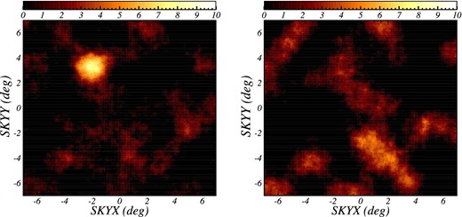
(Left) Significance map around Swift J1644+58 (left upper source) obtained from the data integrated for 30 d when the object was the brightest. (Right) The same, but obtained from the total 37-month data. (Color online)
On the basis of positional coincidence, we identify three TDE candidates in the MAXI transient source catalog from the literature; Swift J1112.2−8238 (hereafter Swift J1112−82; Brown et al. 2015), Swift J1644+57 (Burrows et al. 2011), and Swift J2058.4+0516 (hereafter Swift J2058+05; Cenko et al. 2012). They are located at z = 0.89, z = 0.354, and z = 1.1853, and their (isotropic) luminosities in the 4–10 keV band are estimated to be 1047.1 erg s−1, 1046.6 erg s−1, and 1047.5 erg s−1, respectively. We also identify another candidate that occurred in NGC 4845 (Nikołajuk & Walter 2013), which has been already listed in the 2nd MAXI/GSC catalog (Hiroi et al. 2013). Its 30 d averaged peak flux in the 4–10 keV band is 3.2 mCrab, with a significance of sD = 6.8, which corresponds to a luminosity of 1042.3 erg s−1 at z = 0.004110. We, however, note that the X-ray flare of NGC 4845 may be attributed to a variable AGN, which is supported by the radio observation of the unresolved central core (Irwin et al. 2015). From the time evolution of the radio spectrum, Irwin et al. (2015) also suggested the presence of an expanding outflow or a jet, which may be associated with the X-ray flare. It is not yet clear whether the X-ray flare is due to a TDE or the AGN. The detailed information of each TDE from the literature (Burrows et al. 2011; Cenko et al. 2012; Nikołajuk & Walter 2013; Zauderer et al. 2013; Brown et al. 2015; Pasham et al. 2015) is summarized in table 1.
Our sample of tidal disruption events.*
| Name | z | log L4–10keV | Γ | δ | M * |
|---|---|---|---|---|---|
| [1] | [2] | [3] | [4] | [5] | [6] |
| Swift J1112.2−8238 | 0.89 | 47.1 | — | — | — |
| Swift J164449.3+573451 | 0.354 | 46.6 | 10 | 16 | 0.15 |
| Swift J2058.4+0516 | 1.1853 | 47.5 | >2 | — | 0.1 |
| NGC 4845 | 0.004110 | 42.3 | — | — | 0.02 |
*Col. [1]: name of the TDE. Col. [2]: redshift. Col. [3]: luminosity (erg s−1) in the 4–10 keV band. Col. [4]: the Bulk Lorentz factor. Col. [5]: the Doppler factor. Col. [6]: accreted mass in units of solar mass.
2.3 Search for unidentified TDEs
To constrain statistical properties of TDEs, such as the occurrence rate, as a function of X-ray luminosity (i.e., XLF), it is very important to perform their complete survey at a given flux limit. Hence, we search for other possible TDEs that are not reported in the literature. We make use of the general characteristics of the light curve pattern of TDEs. As mentioned in section 1, a TDE shows a rapid flux increase followed by a power-law decay with an index of −5/3 as a function of time (Rees 1988; Phinney 1989).
For this purpose, we make the light curves of all sources in the 2nd MAXI/GSC catalog (Hiroi et al. 2013) and in the transient catalog (appendix 1) in 10, 30, and 90 d bins, in three energy bands, 3–4 keV, 4–10 keV, and 3–10 keV. The fluxes in individual time-bins are obtained by the same image fitting method as described in appendix 1 by fixing the source positions. We discard the data when the photon statistics are too poor within each bin [see subsection 2.1 in Isobe et al. (2015) for details]. Using the light curve of the Crab nebula analyzed in the same way, we estimate a systematic uncertainty in the flux of ∼10%, which is added to the statistical error.
As a reference, we analyze the light-curve pattern of the four identified TDEs, Swift J1112−82, Swift J1644+57, Swift J2058+05, and NGC 4845. We find that all of them show the following two characteristics. The first one is high variability amplitudes: the ratios between the highest flux and the one of the previous bin in the 30 d (90 d) averaged light curves for Swift J1112−82, Swift J1644+57, Swift J2058+05, and NGC 4845 are 7.0 (1.6), 16.3 (7.7), 8.2 (2.4), and 1.4 (6.8), respectively. Here, we assign a flux of 5 × 10⁻¹² erg s−1 cm−2 (4–10 keV) for each bin when the source is undetected, which is the sensitivity limit of the 2nd MAXI catalog (Hiroi et al. 2013). The second characteristic is that the decay light curves are consistent with a power-law profile of t−5/3, where t is time since the onset time of each TDE. We note that the time of the flux peak, tp, is delayed from the TDE onset time by approximately 80 d for NGC 4845, 20 d for Swift J1644+57 and Swift J2058+05, and 5 d for Swift J1112−82. Hence, we set the central day of the bin showing the highest flux as tp, and estimate the TDE onset time by correcting for these offsets. We confirm that the 10 d light curves in the 3–10 keV band follow power-law profiles, as shown in figure 2. A power-law fit to the light curve over 90 d after the peak flux is found to be acceptable in terms of a χ2 test, yielding the best-fitting indices of |$-1.86^{+0.45}_{-1.55}$|, |$-1.94^{+0.39}_{-0.48}$|, |$-1.92^{+0.58}_{-0.73}$|, and |$-2.00^{+1.14}_{-1.25}$| for Swift J1112−82, Swift J1644+57, Swift J2058+05, and NGC 4845. The errors denote statistical ones at 90% confidence limits, and they are all consistent with −5/3. Accordingly, we apply the above two conditions to the light curves of all MAXI sources (506 in total) except for the four TDEs. First, we find 12 (12) objects which satisfy the criterion that the ratio between the highest and second highest flux bins is larger than 5 in the 30 d (90 d) light curve. For these candidates, we then perform the same light-curve fitting with a power-law profile as described above. The time delay from the TDE onset to the observed flux peak is set to either 5 d, 20 d, or 80 d. As a result, we find that none of them show a decaying index consistent with −5/3 except for the objects identified as AGNs or X-ray galactic sources. Thus, we conclude that MAXI detected only the four TDEs identified above during the first 37 months of its operation, which can be regarded as a statistically complete sample at the sensitivity limit of MAXI for transient events, as long as TDEs share similar characteristics in the X-ray light curve to those of the known events. According to numerical simulations, the index of the power-law decay becomes steeper than −5/3 when the star is not fully disrupted (Guillochon & Ramirez-Ruiz 2013). Such events would be missed in our sample. We find that the four TDE candidates reported by Hryniewicz and Walter (2016) from the Swift/BAT ultra-hard X-ray band (20–195 keV) data were not significantly detected in the MAXI data that covered the same epoch. The details are given in appendix 2. In all events, the flux upper limit in the MAXI band is smaller by a factor of ∼4 than that expected from the Swift/BAT flux by assuming a photon index of 2.0. This implies that these TDE candidates might have unexpectedly hard spectra or be subject to heavy obscuration. Such TDEs, if any, are not considered in our analysis.
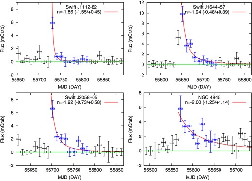
X-ray (3–10 keV) light curves of four TDEs during their flares. A power-law decay model is fitted to only blue regions. The best-fitting power-law index (n) is indicated in each panel, with errors at 90% confidence level. (Color online)
The continuous monitoring data of MAXI provide us with unique information on the X-ray light curve of TDEs in the 3–10 keV band, which can be compared with those obtained with Swift/BAT in the 14–195 keV band. Figure 3 plots the MAXI light curves in 1 d bins of the three TDEs excluding NGC 4845, which was too faint to be examined on shorter time scales than 10 d. We find that the luminosities for Swift J1112−82, Swift J2058+05, and Swift J1644+57 peaked at MJD = 55729, MJD = 55649, and MJD = 55701, respectively, which are all consistent with those determined with Swift/BAT within 1 d (Burrows et al. 2011; Cenko et al. 2012; Brown et al. 2015). Thus, there is no evidence for significant (>1 d) time lags between the soft (<10 keV) and hard (>10 keV) bands.
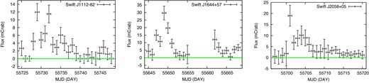
X-ray (3–10 keV) light curves of the three TDEs with relativistic jets around their peak luminosities in 1 d bins. For Swift J1644+57 no MAXI data were obtained around MJD ∼55660. (Color online)
3 Hard X-ray luminosity function of tidal disruption events
3.1 Definition of luminosities
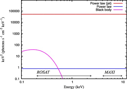
Representative spectrum of a TDE with Tbb = 5 × 10⁵ K. The three components are shown (red: jet component with δ = 16; blue: Comptonized component; magenta: blackbody component). The unit of the vertical axis is arbitrary. (Color online)
3.2 TDE sample
We regard the four identified TDEs listed in table 1 as constituting a complete sample from the MAXI survey during 37 months, and we utilize them to derive the XLF. When integrated over 30 d, the MAXI survey covers all the high Galactic latitudes (|b| > 10°) region, which corresponds to 83% of the entire sky. As described in the previous subsection, we have searched for TDEs based on 30 d or 90 d binned light curves. Thus, the sensitivity limit for the 30 d averaged peak flux of TDEs where our sample becomes the flux limited one is determined by that for 30 d integrated data of MAXI/GSC, which is 2.5 mCrab, or 3 × 10⁻¹¹ erg s−1 cm−2 (4–10 keV). For simplicity, we ignore the dependence of the sensitivity on sky positions (Hiroi et al. 2013), whose effects are much smaller than the statistical uncertainties in the XLF parameters.
It is necessary to assume a spectrum to derive the luminosity from the observed count rate of MAXI/GSC. Because the blackbody component can be ignored in the 4–10 keV band, here we assume a power-law spectrum absorbed with the hydrogen column-densities reported by the previous studies (Burrows et al. 2011; Cenko et al. 2012; Nikołajuk & Walter 2013; Brown et al. 2015). In the following analysis, for simplicity, we always adopt a photon index of 2 for both Comptonization and jet components, as a representative value. In fact, for all four TDEs, the hardness ratio defined as (H − S)/(H + S), where H and S are the count rates obtained from the MAXI data in the 4–10 keV and 3–4 keV bands, respectively, is consistent with a photon index of 2.0 within uncertainties. In this case, the K-correction factor is always unity and ωpow = ωjet. The calculated peak luminosity of each TDE is listed in table 1. Its systematic error due to the uncertainty in the peak-flux time within the bin size of the MAXI light curve has negligible effect on our conclusions.
3.3 Formulation of TDE X-ray luminosity function
We define the XLF of TDEs so that dΦ(LX, z)/dLX represents the TDE occurrence rate per unit co-moving volume per LX per unit rest-frame time, as a function of LX and z, in units of Mpc|$^{-3}\,L_{\rm X}^{-1}\:$|yr−1. Note that this function has an additional dimension of per unit time compared with the “instantaneous” XLF of TDEs and the XLF of AGNs (see subsection 4.3), which represents the number densities of TDEs and AGNs, respectively, observed in a single epoch.
3.4 Mass function of stars disrupted by SMBHs
3.5 Maximum likelihood fit
We adopt the unbinned maximum likelihood (ML) method to constrain the XLF parameters. While the ML fit gives the best-fitting parameters, the goodness of the fit cannot be evaluated. Hence, we perform a one-dimensional Kolmogorov–Smirnov test (hereafter KS test, e.g., Press et al. 1992) separately for the redshift distribution and for the luminosity distribution between the observed data and the best-fitting model. The p-value, the chance of getting observed data set, is evaluated from the D-value assuming the one-sided KS test statistic. The D-value is chosen as the maximum value among the absolute distances between an empirical cumulative distribution function and a theoretical one.
Since our sample size of TDEs is very small (four), we fix the following parameters of the XLF model, which cannot be well constrained from the data. We adopt a characteristic luminosity of log LX* = 44.6 corresponding to the Eddington ratio of λEdd = 1 (see next paragraph). As mentioned previously and listed in table 2, the Lorentz factor of the jets, the dependence of the specific TDE rate on SMBH mass, the fraction of the intrinsic jet luminosity in LX, and the upper mass boundary of tidally disrupted stars are fixed at Γ = 10, λ = −0.4, ηjet = 0.1, and M*, max = 1.0 M⊙ as the standard parameters, respectively. Effects on the main results by changing these numbers (λEdd, Γ, λ, ηjet, and M*, max) from the default values will be examined in subsections 3.6 and 3.7. The index of the redshift evolution is assumed to be either p = 0 (no evolution case) or 4 (strong evolution case). According to the prediction of numerical simulations that the occurrence rate of TDEs increases with the star-formation rate (Aharon et al. 2016), the latter case simply assumes that the TDE rate is proportional to the star-formation rate density, which evolves with ∝(1 + z)4 (Pérez-González et al. 2005). Eventually, only ϕ0ξ0 and fjet are left as free parameters.
Default setting of fixed parameters.*
| λEdd | Γ | λ | ηjet | M *, max |
|---|---|---|---|---|
| [1] | [2] | [3] | [4] | [5] |
| 1.0 | 10 | −0.4 | 0.1 | 1.0 |
| λEdd | Γ | λ | ηjet | M *, max |
|---|---|---|---|---|
| [1] | [2] | [3] | [4] | [5] |
| 1.0 | 10 | −0.4 | 0.1 | 1.0 |
*Col. [1]: Eddington ratio. Col. [2]: the Lorentz factor. Col. [3]: index for the MBH dependence of the TDE rate. Col. [4]: fraction of the intrinsic luminosity of the jet in LX. Col. [5]: upper mass boundary of disrupted stars in units of solar mass.
The minimization procedure is carried out by using the MINUIT software package. We calculate the likelihood function over a redshift range of z = 0–1.5. The luminosity range is derived from the SMBH range of log (MBH/M⊙) = 4–8 for a given λEdd (1.0). To convert the mass into the X-ray luminosity LX, we consider a spectrum composed of the three components described in subsection 3.1 (the blackbody, Comptonization, and jet components). Specifically, we first determine the ratio of the Comptonized component in the 2–10 keV band to the bolometric luminosity without a jet component. Assuming that accretion physics in TDEs is similar to that of AGNs, we refer to the results by Vasudevan and Fabian (2007), who derived from the 2–10 keV band a bolometric correction factor (k2–10) of ∼50 for λEdd = 1.0. We then convert the luminosity in the 2–10 keV band into that in the 4–10 keV band by assuming a power-law photon index of 2.0. As a result, log LX shows a range from 40.2 to 44.2 for λEdd = 1.0. The rest of the bolometric luminosity is attributed to the blackbody emission. The integration range of M* is determined to satisfy the criterion RTDE/RSch ≥ 1. To calculate the tidal disruption radius RTDE = R*(MBH/M*)1/3, we convert the radius of a disrupted star R* into a mass M* with R*/R⊙ = (M*/M⊙)0.8 (e.g., Kippenhahn & Weigert 1990). Hence, RTDE/RSch is a function of M* and MBH, or that of M*, λEdd, and LX.
Table 3 summarizes the results of the ML fit for the cosmological evolution indices of p = 0 and p = 4. The other fixed parameters are also listed in table 2. One-dimensional KS tests for the distribution of z and for that of |$L^{\rm obs}_{\rm X}$| do not rule out either result at the 90% confidence level. The 90% confidence upper and lower limits on fjet are derived, corresponding to the case where the |$\mathcal {L}$|-value is increased by 2.7 from its minimum. Since the ML method cannot directly determine the normalization (ψ0ξ0) of the luminosity function, we calculate it so that the predicted number from the model equals the detected number of the TDEs. The attached error corresponds to the Poisson error in the observed number at the 90% confidence level based on equations (9) and (12) in Gehrels (1986).
Best-fitting parameters.*
| p | f jet | ψ0ξ0 | p-value (|$L^{\rm obs}_{\rm X}$|-distr./z-distr.) |
|---|---|---|---|
| [1] | [2] | [3] | [4] |
| 0 | 0.012|$^{+0.122}_{-0.010}$| | |$1.7^{+1.6}_{-0.9}$| | 0.16/0.14 |
| 4 | 0.003|$^{+0.027}_{-0.002}$| | |$1.6^{+1.6}_{-0.9}$| | 0.60/0.40 |
| p | f jet | ψ0ξ0 | p-value (|$L^{\rm obs}_{\rm X}$|-distr./z-distr.) |
|---|---|---|---|
| [1] | [2] | [3] | [4] |
| 0 | 0.012|$^{+0.122}_{-0.010}$| | |$1.7^{+1.6}_{-0.9}$| | 0.16/0.14 |
| 4 | 0.003|$^{+0.027}_{-0.002}$| | |$1.6^{+1.6}_{-0.9}$| | 0.60/0.40 |
*Col. [1]: Index of the redshift evolution. Col. [2]: Fraction of the TDEs with jets. Col. [3]: Normalization factor of XLF in units of 10−8 Mpc−3|$\log L_{\rm X}^{-1}\:$|yr−1. Col. [4]: p-value on the basis of the KS-test for each parameter of |$L^{\rm obs}_{\rm X}$| and z.
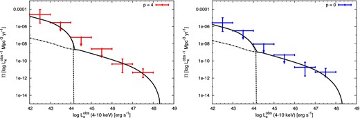
Best-fitting XLF as a function of “observed” peak luminosity at z = 0.75 for two evolution indices (left-hand panel: p = 4; right-hand panel: p = 0). The solid lines represent the total XLF consisting of that of TDEs without jets (dotted line) and that of TDEs with jets (dot–dashed line). (Color online)
Table 4 lists the TDE occurrence rates per unit volume (Mpc−3 yr−1) in different luminosity ranges predicted from our best-fitting TDE XLFs. The corresponding errors are calculated by only considering the uncertainty in the normalization of the TDE XLF.
Frequency of TDE occurrence at different luminosity ranges.*
| log |$L^{\rm obs}_{\rm X}$| | |$\dot{N}_{p = 0}$| | |$\dot{N}_{p = 4}$| |
|---|---|---|
| [1] | [2] | [3] |
| 40–41 | |$1.2^{+1.2}_{-0.7}\times 10^{-5}$| | |$1.1^{+1.1}_{-0.6}\times 10^{-5}$| |
| 41–42 | |$4.0^{+4.0}_{-2.3}\times 10^{-6}$| | |$3.8^{+3.8}_{-2.2}\times 10^{-6}$| |
| 42–43 | |$9.0^{+9.0}_{-5.1}\times 10^{-7}$| | |$8.6^{+8.6}_{-4.8}\times 10^{-7}$| |
| 43–44 | |$1.2^{+1.2}_{-0.7}\times 10^{-7}$| | |$1.1^{+1.1}_{-0.6}\times 10^{-7}$| |
| 44–45 | |$1.1^{+1.1}_{-0.6}\times 10^{-9}$| | |$4.8^{+4.7}_{-2.7}\times 10^{-10}$| |
| 45–46 | |$1.8^{+1.8}_{-1.0}\times 10^{-10}$| | |$3.8^{+3.8}_{-2.2}\times 10^{-11}$| |
| 46–47 | |$3.1^{+3.1}_{-1.8}\times 10^{-11}$| | |$6.6^{+6.6}_{-3.7}\times 10^{-12}$| |
| 47–48 | |$2.6^{+2.5}_{-1.4}\times 10^{-12}$| | |$5.4^{+5.4}_{-3.1}\times 10^{-13}$| |
*Col. [1]: Luminosity range. Col. [2]: Frequency of the TDE occurrence (Mpc−3 yr−1) in the corresponding luminosity range for log LX* = 44.6 and p = 0. Col. [3]: Same as Col. [2] but for p = 4.
3.6 Comparison with ROSAT results
We check the consistency between our results and a previous study based on the ROSAT All-Sky Survey (RASS: Donley et al. 2002). Here, we must take into account the different TDE survey conditions between MAXI and ROSAT. Because MAXI is continuously monitoring the entire sky, we can derive the whole light-curve of each TDE and hence its “peak” luminosity. By contrast, the detection of TDEs reported by the ROSAT survey was based on two snapshot observations, one in the scanning mode during the RASS and the other in the pointing mode. Thus, in the case of ROSAT, it is impossible to accurately estimate the “peak” luminosity of each TDE because of the uncertainty in its peak flux time due to the scarcity of the observations.
To perform this calculation, we need C0 and C1, the conversion factors from an intrinsic luminosity to an observed luminosity in the ROSAT band (0.2–2.4 keV). Since the blackbody component can be dominant in this energy band, the terms of ωbb in equations (3) and (4) must be estimated. We follow our assumption that the rest of the non-beamed bolometric luminosity from which the Comptonization component is subtracted is dominated by a blackbody component with a single temperature. Accordingly, we estimate the effective temperature by assuming that the emitting area of the blackbody component is ∼π(3RSch)2. The color temperature is assumed to be identical to the effective one. As a result, ωbb is derived as a function of LX and z. We obtain ωpow = 2.71 for a power-law photon index of 2.0.
When comparing the ROSAT and MAXI results, we should take into account the fact that the RASS performed in the soft X-ray band would easily miss obscured TDEs, unlike the case of MAXI. Indeed, the follow-up observations of our four TDEs with Swift or XMM-Newton indicate that two of them (Swift J1644+57 and NGC 4845; Burrows et al. 2011; Nikołajuk & Walter 2013) are obscured by column densities of NH > 1022 cm−2. From this result, we estimate the obscuration fraction to be ∼1/2, and, accordingly, decrease the detectable number of TDEs NTDE by a factor of 2 to be compared with the ROSAT result. Also, we implicitly assume that all TDEs have hard X-ray components. Although they are not significantly required in the RASS spectra of WPVS 007 (Grupe et al. 1995) and RX J1624.9+7554 (Grupe et al. 1999), their expected contribution to the 0.5–2 keV flux can be very small (∼1%) and hence cannot be well constrained with these data owing to the limited energy band and photon statistics. To confirm this assumption, future broadband observations of TDEs, like those by eROSITA, will be important.
We calculate NTDE using equation (20) from our best-fitting XLF models summarized in table 3. We obtain |$N_{\rm TDE}/2 = 3.2^{+3.2}_{-1.8}$| for p = 0 and |$N_{\rm TDE}/2 = 4.0^{+3.9}_{-2.2}$| for p = 4, which are consistent with the observed number of TDEs (three or two) in the ROSAT survey. When λEdd = 0.1 (corresponding to log LX* = 44.0) is adopted instead of λEdd = 1.0 (log LX* = 44.6), the derived XLF predicts |$N_{\rm TDE}/2 = 0.7^{+0.7}_{-0.4}$| for p = 0 and |$N_{\rm TDE}/2 = 1.2^{+1.2}_{-0.7}$| for p = 4. These numbers are significantly smaller than three at the 90% confidence level, although that for p = 4 is consistent with the two (i.e., when the event in IC 3599 is excluded from the ROSAT sample). Also, under the assumption of λEdd = 5 and k2–10 = 70 as a super-Eddington accretion case, the predicted TDE number is significantly higher (NTDE/2 ≳ 4) than the observed one regardless of the evolution index (p). Hence, we adopt λEdd = 1.0 in our baseline model, which is allowed for the range of p = 0–4.
In the above calculations of NTDE, we have ignored the possible time evolution of the X-ray spectrum of each TDE during the decay phase. According to Vasudevan and Fabian (2007), the bolometric correction factor from the 2–10 keV band (k2–10) depends on the Eddington ratio. Since k2–10 determines the relative weights between the Comptonized and blackbody components in our assumption, the X-ray spectrum is predicted to be time-dependent. To roughly examine these effects, we calculate NTDE approximating that k2–10 = 50 for λEdd ≥ 0.1 and k2–10 = 20 for λEdd < 0.1. In the case of λEdd = 1.0, we obtain |$N_{\rm TDE}/2 = 3.7^{+3.7}_{-2.1}$| for p = 0 and |$N_{\rm TDE}/2 = 4.8^{+4.8}_{-2.7}$| for p = 4, while NTDE/2 < 3 is obtained for both p = 0 and 4 in the case of λEdd = 0.1. Hence, the possible spectral evolution does not affect our conclusion.
3.7 Effects by changing fixed parameters
In this subsection, we examine the effects on the XLF results, particularly fjet, by changing the fixed parameters in the XLF model that are difficult of constraint on the data: (1) the Lorentz factor of the jets (Γ); (2) the dependence of the specific TDE rate on SMBH mass (λ); (3) the fraction of the intrinsic jet luminosity in LX (ηjet); (4) the upper mass boundary of tidally disrupted stars (M*, max). Considering the small sample size, we perform an ML fit of the XLF by adopting an alternative value instead of the default value for each fixed parameter and check how fjet is affected. We consider Γ = 5 and 20 (default is 10), λ = −0.1 (default is −0.4), ηjet = 0.01, 1.0, and 10.0 (default is 0.1), and M*, max/M⊙ = 10 and 100 (default is 1). In each case, we assume the two evolution indices, p = 0 and p = 4. We regard the minimum or maximum values considered here as corresponding to extreme cases within physically plausible values.
Figure 6 summarizes the constraints on fjet plotted against Γ when one of the other parameters (λ, ηjet, M*, max) is changed. The red and blue marks correspond to p = 0 and p = 4, respectively. If an acceptable fit is not obtained in terms of the one-dimensional KS tests (for the redshift and luminosity distributions) and/or the predicted number of TDEs in the ROSAT survey, we mark them in gray. Also, when the maximum luminosity in the TDE XLF is lower than the observed one (log LX = 47.5), we plot the points at the position of fjet = 100% in gray. These gray points should be ignored because the corresponding XLF model is rejected.
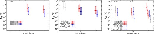
Constraint on fjet plotted against the jet Lorentz factor Γ for various choices of the other parameters in the XLF (λ, M*, max, ηjet). For clarity, the data points are slightly shifted along the x-axis. The gray points correspond to the case where the fit is rejected in terms of the one-dimensional KS tests (for the redshift and/or luminosity distributions), and/or the predicted number of TDEs in the ROSAT survey. Also, we plot the points at the position of fjet = 100% in gray when the TDE XLF cannot reproduce the observed maximum luminosity (log LX = 47.5). Hence, these gray points should be ignored. (Color online)
Among the acceptable parameter sets, we obtain the maximum upper limit of fjet = 34% for Γ = 20, ηjet = 0.01, and p = 0, and the minimum lower limit of fjet = 0.0007% for Γ = 10, ηjet = 10.0, and p = 4. Thus, we conservatively estimate that the fraction of TDEs with jets among all TDEs is 0.0007%–34%. This constraint is compatible with the fraction of radio-loud AGNs in all AGNs (∼10%). We note that fjet depends on a combination of ηjet and Γ. This is mainly because the cut-off luminosity of the XLF for TDEs with jets is determined as ηjetδ(Γ, θ)4, with which fjet is strongly coupled: one obtains a large value of fjet when ηjet and/or Γ becomes smaller. Since Γ determines the solid-angle of the detectable relativistic jets (∝1/Γ2), there is another coupling of fjet with Γ, which partially cancels out the coupling through the cut-off luminosity.
4 Discussions
4.1 Result summary
Utilizing a complete sample of TDEs detected in the MAXI extragalactic survey in the 4–10 keV band, we have, for the first time, quantitatively derived the shape of the XLF of TDEs (the occurrence rate of a TDE per unit volume) as a function of intrinsic peak luminosity at z ≲ 1.5. We take account of two TDE types of XLF, one with jets and the other without jets, and those subject to heavy absorption that would be difficult of detection in soft X-ray surveys. In the modeling of the XLF, we have taken into account the mass function of SMBHs, that of disrupted stars, the specific TDE rate as a function of SMBH mass, and relativistic beaming effects from jets, although we need to fix several parameters at reasonable values. The XLF can be converted to an “instantaneous XLF” obtained from a single-epoch observation in different energy bands, by assuming spectra of TDEs. Our baseline model, whose parameters are listed in table 2, is found to reproduce the number of TDEs previously detected in the ROSAT survey well. The main finding is that the fraction of TDEs with jets among all TDEs is 0.0007%–34%. Our result will serve as a reference model of a TDE XLF, which would be useful for estimating their contribution to the growth history of SMBHs and for predicting TDE detections in future missions.
4.2 Comparison of TDE rate with previous studies
We compare the TDE rate per unit volume based on our best-fitting XLF with those estimated from previous studies. Combining the XMM-Newton slew survey and the RASS, Esquej et al. (2008) detected two TDEs, whose soft X-ray luminosities were ∼5 × 1041 erg s−1 and ∼5 × 1043 erg s−1. They derived a TDE rate per unit volume of ∼5 × 10⁻⁶ Mpc−3 yr−1 for the peak luminosity of 1044 erg s−1 in the 0.2–2.0 keV band. In table 4 we predict the rate of unobscured TDEs with the peak luminosity >1041 erg s−1 (4–10 keV) to be ∼5 × 10⁻⁶ Mpc−3 yr−1 at z = 0, which is in good agreement with the estimate made by Esquej et al. (2008).
Maksym, Ulmer, and Eracleous (2010) studied a TDE in the galaxy cluster Abell 1689, using Chandra and XMM-Newton. The TDE rate “per galaxy” was estimated to be 6 × 10⁻⁵ galaxy−1 yr−1 for the minimum luminosity in the 0.3–2.5 keV band of 1042 erg s−1. Our XLF predicts a TDE rate of ∼1 × 10⁻⁴ galaxy−1 yr−1 for peak luminosities of log LX > 42, by adopting the spatial density of galaxies of ϕ0 = 0.007 galaxy Mpc−3. As mentioned in Maksym, Ulmer, and Eracleous (2010), the discrepancy by a factor of ∼2 may be explained if only half the number of member galaxies in Abell 1689 can produce TDEs detectable by their analysis.
It is interesting to compare our TDE rate with that obtained from the flux-complete, optically selected sample of van Velzen and Farrar (2014) using archival Sloan Digital Sky Survey data. They detected two TDE candidates, and estimated the TDE rate of ∼(4–8) × 10−8 Mpc−3 yr−1 for SMBH masses of ∼107 M⊙. Our estimate for the corresponding luminosity (log LX ≳ 43) is ∼1 × 10⁻⁷ Mpc−3 yr−1. This is higher than the TDE rate of van Velzen and Farrar (2014). It may be owing to dust extinction, which reduces the number of TDE flares detectable in the optical band. Indeed, if we correct the optical TDE rate for obscuration by a factor of 2, it becomes ∼(8–16) × 10−8 Mpc−3 yr−1, which is consistent with the X-ray result.
4.3 Contribution of TDEs to X-ray luminosity functions of AGNs
It is possible that the XLF of AGNs may be contaminated by TDEs, which are difficult to distinguish from AGNs in observations of limited numbers. To investigate this effect, we calculate the instantaneous XLFs of TDEs based on our best-fitting parameters using equation (18). Figure 7 plots the results in the 2–10 keV band at the low redshift (0.002 < z < 0.2) and high redshift (1.0 < z < 1.2) ranges for the two evolution indices, p = 0 and p = 4. The error region at the 90% confidence level due to the uncertainty in the normalization is also indicated. The luminosity range below the sensitivity limit where the TDE XLF is not directly constrained by the MAXI survey is indicated by the dashed lines.
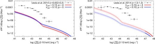
Comparison of the instantaneous XLF of TDEs (our work) and the XLF of AGNs (Ueda et al. 2014) in the 2–10 keV band. The left-hand and right-hand panels show the results in the low (z = 0.1) and high (z = 1.1) redshift ranges, respectively. Each line is colored in accordance with the notation in the figure. The 1σ Poisson errors are attached to the AGN XLF. (Color online)
For comparison, we overplot the hard XLF of AGNs obtained by Ueda et al. (2014) at z = 0.1 and z = 1.1 for the two redshift ranges. As noticed from figure 7, the instantaneous XLF of TDEs are far below the observed AGN XLF at 0.002 < z < 0.2, indicating that the contribution of TDEs is negligible in the local universe. At 1.0 < z < 1.2, the TDE contribution to the AGN XLF is also negligible at high luminosities, while it could be significant in the lowest luminosity range. However, the model of the TDE XLF in this region is just an extrapolation from the result in the low-redshift range, and must be constrained by more sensitive surveys to reach any conclusions.
4.4 Mass accretion history of SMBHs by TDEs
We adopt the mass-to-radiation conversion efficiency of ϵ = 0.1, similarly in the case of AGNs. Figure 8 shows the cumulative SMBH mass-density (M⊙ Mpc−3) calculated from zs = 1.5. We find that the total mass density at z = 0 is at most 7 × 10² M⊙ Mpc−3 even in the case of p = 4. This indicates that the SMBH mass-density contributed by TDEs is much less than that of AGNs (e.g., Ueda et al. 2014). This is what is expected from the comparison in XLF between TDE and AGN as described in the previous subsection.
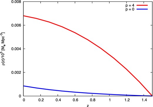
Evolution of SMBH mass-density caused by TDEs. Each line is colored in accordance with the notation in the figure. (Color online)
5 Summary
We have derived the XLF of TDEs, i.e., the occurrence rate of a TDE per unit volume as a function of intrinsic peak luminosity, from the MAXI extragalactic survey. Our sample consists of four TDEs, Swift J1112−82, Swift J1644+57, Swift J2058+05, and NGC 4845, detected in the first 37 months’ data of MAXI/GSC at high Galactic latitudes (|b| > 10°). It is complete up to a flux limit of ∼3 × 10⁻¹¹ erg s−1 cm−2 (4–10 keV), and is less affected with absorption than those detected in lower energy bands. In fact, two TDEs out of the four show significant absorptions in the X-ray spectra.
We formulate the shape of the TDE XLF, based on the mass function of SMBHs, that of tidally disrupted stars, and the specific TDE rate as a function of SMBH mass. We take account of two distinct types of TDEs, XLF with jets and XLF without jets, and also of the relativistic beaming from the jets. To incorporate effects of the cosmological evolution, we assume two cases where the XLF is constant over redshift or proportional to (1 + z)4. ML fits are performed to the observed TDE sample, with the normalization of the XLF (i.e., TDE rate) and the fraction of TDEs with jets among all TDEs, fjet, allowed to vary. We then verify the best-fitting model by checking consistency between our sample and the ROSAT study by Donley et al. (2002). Consequently, we find that fjet is constrained to be 0.0007%–34%, consistent with the case of AGNs.
On the basis of our best-fitting TDE XLF, we have estimated the contributions of TDEs to instantaneous XLFs of AGNs and to the evolution of the SMBH mass density. It is found to be much smaller than those of AGNs, indicating that the effect of TDEs on the growth of SMBHs is negligible at z ≲ 1.5. Future observations of TDEs, including the eROSITA survey, will enable us to establish more accurate statistical properties of TDEs over wide luminosity and redshift ranges.
Part of this work was financially supported by the Grant-in-Aid for JSPS Fellows for young researchers (TK, MS) and for Scientific Research 26400228 (YU). This research has made use of MAXI data provided by RIKEN, JAXA and the MAXI team.
Appendix 1. Detection of X-ray transient events from MAXI data
This section describes the image analysis of the MAXI/GSC data employed to extract the transient X-ray events. The method is essentially the same as that of Hiroi et al. (2013) used for producing the 37-month catalog, but is applied to 37 (or 12) individual images binned in 30 d (or 90 d) to obtain the light curves of all sources including newly detected transient objects.
The entire all-sky image in each time-bin is divided into 768 areas of 14° × 14° size centered at the coordinates defined in the HEALPix software (Górski et al. 2005). Circular regions around the very bright sources Sco X-1, Cyg X-2, and Crab Nebula are not used in our analysis to avoid systematic errors in the calibration of the point spread function (PSF). First, combining the observed image and the model of the background (the cosmic X-ray background plus the non-X-ray background), we make the significance map: an example is shown in figure 1. Here the significance at each position is simply calculated as the background-subtracted counts divided by the square root of total counts in the 0| $_{.}^{\circ}$|1 × 0| $_{.}^{\circ}$|1 region around it. Then, excess points with the peak significance above 5.5σ are left as source candidates. We regard those whose positions do not match any sources in the 37-month MAXI/GSC catalog within 1° as candidates of transient sources newly detected in this time-sliced image analysis.
To determine the fluxes of all source candidates, we then perform image fitting with a model composed of the background and PSFs. Here we consider PSFs of all sources in the 37-month MAXI catalog and those of the transient candidates extracted above. The PSFs are calculated using the MAXI simulator (Eguchi et al. 2009) by assuming the spectrum of the Crab nebula. The fluxes of all sources (in units of Crab) and the normalization of the background are left as free parameters. The positions of the 37-month MAXI catalog sources are fixed according to the results by Hiroi et al. (2013), while those of the transient candidates are set to free parameters. To find the best-fitting parameters and their statistical errors, we employ the maximum likelihood algorithm based on the C statistics (Cash 1979), utilizing the MINUIT software package. To ensure complete detections of transient events, we repeat the above procedures twice for each image. Namely, we again make the significance map based on the best-fitting model including the PSFs, search for remaining residuals with the significance above 5.5σ, and then perform the image fitting including new source candidates.
The results are that we detect 10 transient events in total at high galactic latitudes (|b| > 10°), whose detection significance exceeds 5.5 in either of the analyzed images. Here we have paid careful attention to excluding fake events caused by light contamination from the Sun by checking the image and spectra. Table 5 summarizes the basic information about the events. The parameters are derived from an image where the event was detected with the highest detection significance among all time-bins.
Information on transient events.*
| MAXI name | RA | Dec | σpos | s D | f 4–10keV | Hardness ratio | Flare time | Counterpart | Type |
|---|---|---|---|---|---|---|---|---|---|
| [1] | [2] | [3] | [4] | [5] | [6] | [7] | [8] | [9] | [10] |
| 2MAXIt J0745−504 | 116.451 | −50.496 | 0.216 | 6.07 | 5.16 | >0.87 | 55727–55756 | HD 63008 | Star |
| 2MAXIt J1108−829 | 167.064 | −82.914 | 0.191 | 6.70 | 2.88 | 0.19 ± 0.14 | 55727–55756 | Swift J1112.2−8238 | Tidal disruption event |
| 2MAXIt J1159+238 | 179.814 | 23.876 | 0.185 | 5.77 | 2.66 | >0.71 | 55877–55906 | ||
| 2MAXIt J1507−217 | 226.882 | −21.743 | 0.122 | 10.35 | 8.59 | 0.33 ± 0.11 | 55127–55156 | GRB 091120 | Gamma-ray burst |
| 2MAXIt J1517+067 | 229.350 | 6.793 | 0.198 | 5.79 | 1.79 | 0.23 ± 0.18 | 55637–55726 | ||
| 2MAXIt J1645+576 | 251.379 | 57.604 | 0.131 | 8.83 | 3.18 | 0.18 ± 0.12 | 55637–55726 | Swift J164449.3+573451 | Tidal disruption event |
| 2MAXIt J1807+132 | 271.806 | 13.269 | 0.184 | 5.68 | 2.73 | 0.28 ± 0.18 | 55697–55726 | ||
| 2MAXIt J1944+022 | 296.170 | 2.203 | 0.219 | 6.12 | 2.45 | <0.32 | 55997–56086 | Swift J1943.4+0228 | CV |
| 2MAXIt J2058+053 | 314.578 | 5.377 | 0.202 | 6.39 | 3.39 | 0.19 ± 0.15 | 55697–55726 | Swift J2058.4+0516 | Tidal disruption event |
| 2MAXIt J2313+030 | 348.455 | 3.037 | 0.223 | 6.01 | 4.09 | <0.23 | 55097–55126 | SZ Psc | RS CVn |
*Col. [1]: MAXI name. Col. [2]: right ascension, in units of degree. Col. [3]: Declination, in units of degree. Col. [4]: 1σ statistical position error. Col. [5]: detection significance. Col. [6]: Average flux over a time interval in the 4–10 keV band in units of mCrab. Col. [7]: Hardness ratio and its 1σ error. Col. [8]: Epoch (MJD) when the source is detected. The values of Cols. [2]–[7] are derived in this time interval. Col. [9]: name of the counterpart. Col. [10]: type of the counterpart.
To find possible counterparts of our transient events, we check major X-ray source catalogs and the literature regarding gamma-ray bursts and TDEs covering our observation epoch: the Palermo Swift BAT X-ray catalog (Cusumano et al. 2010), the Fermi 2nd LAT Catalog (Nolan et al. 2012), the ROSAT Bright Source Catalog (Voges et al. 1999), the Swift BAT 70-month Catalog (Baumgartner et al. 2013), Swift Transient Monitor Catalog (Krimm et al. 2013), the First XMM-Newton Sky Slew Survey Catalog (Saxton et al. 2008), the INTEGRAL General Reference Catalog (version 36), and papers by Cenko et al. (2012), Zauderer et al. (2013), Serino et al. (2014), and Brown et al. (2015). We identify a counterpart if its position is within the 3σ positional error (corresponding to the 99% confidence level) of a MAXI transient source. The error consists of the statistical and systematic errors, |$\sigma _{\rm pos} = (\sigma _{\rm stat}^2 + \sigma _{\rm sys}^2)^{1/2}$|. Here, the systematic error is chosen as 0| $_{.}^{\circ}$|05 according to the previous studies (Hiroi et al. 2011, 2013). Figure 9 plots the 10 d bin light-curves in the 3–10 keV band of all transient events excluding the three TDEs (Swift J1112−82, Swift J1644+57, and Swift J2058+05).
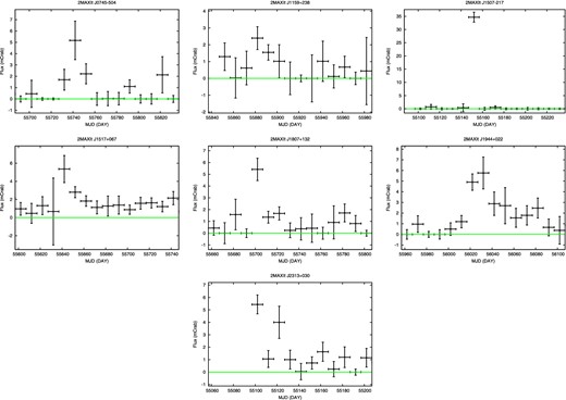
The 10 d bin MAXI light curves in the 3–10 keV band of transient sources excluding the three TDEs. (Color online)
Appendix 2. MAXI results for TDE candidates suggested in the Swift/BAT data
We check if MAXI also found any signals of the TDE candidates reported by Hryniewicz and Walter (2016), who used the Swift/BAT ultra-hard X-ray (20–195 keV) data taken between 2005 and 2013. The number of TDE candidates detected within the 37-month period of our MAXI data is four. We confirm that all of them are not significantly detected in the 4–10 keV image integrated over a 30 d period covering the flare time. Thus, it is justified not to include these events in our analysis. Table 6 summarizes the 5.5σ upper limit of the fluxes in the 4–10 keV band together with the basic information on each TDE. We find that in all events the MAXI upper limit is smaller by a factor of ∼4 than that expected from the averaged BAT flux in the same epoch by assuming a photon index of 2. The reason is unclear, but these events might be subject to heavy (nearly Compton-thick) obscuration.
Information on Swift/BAT TDE candidates.*
| Name | RA | Dec | |$\hat{f}_{\rm 4-10keV}$| | Epoch |
|---|---|---|---|---|
| [1] | [2] | [3] | [4] | [5] |
| PGC 015259 | 67.341 | −4.760 | <1.7 | 55217–55246 |
| UGC 03317 | 83.406 | 73.726 | <1.1 | 55457–55486 |
| PGC 1185375 | 225.960 | 1.127 | <3.5 | 55247–55276 |
| PGC 1190358 | 226.370 | 1.293 | <3.2 | 55247–55276 |
*Col. [1]: Name of TDE candidates detected with Swift/BAT (Hryniewicz & Walter 2016). Col. [2]: Right ascension, in units of degree. Col. [3]: Declination, in units of degree. Col. [4]: 5.5σ upper limit of the averaged 4–10 keV flux in a 30 d period covering the flare time, in units of mCrab. Col. [5]: Epoch (MJD) when the upper flux limit is estimated.
References
