


Abstract
Optical spectropolarimetry by Kishimoto et al. (2004, MNRAS, 354, 1065) has shown that several luminous type 1 quasars show a strong decrease of the polarized continuum flux in the rest-frame near-ultraviolet (UV) wavelengths of λ < 4000 Å. In the literature, this spectral feature is interpreted as evidence of the broadened hydrogen Balmer absorption edge imprinted on the accretion disk thermal emission due to the disk atmospheric opacity effect. On the other hand, quasar flux variability studies have shown that the variable continuum component in UV–optical spectra of quasars, which is considered to be a good indicator of the intrinsic spectral shape of the accretion disk emission, generally has a significantly flat spectral shape throughout the near-UV to optical spectral range. To examine whether the disk continuum spectral shapes revealed as the polarized flux and as the variable component spectra are consistent with each other, we carry out multi-band photometric monitoring observations for a sample of four polarization-decreasing quasars of Kishimoto et al.'s (4C 09.72, 3C 323.1, Ton 202, and B2 1208+32) to derive the variable component spectra and compare the spectral shape of them with that of the polarized flux spectra. Contrary to expectation, we confirm that the two spectral components of these quasars have totally different spectral shapes, in that the variable component spectra are significantly bluer compared to the polarized flux spectra. This discrepancy between two spectral shapes may imply either (1) the decrease of polarization degree in the rest-frame UV wavelengths is not indicating the Balmer absorption edge feature but is induced by some unknown (de)polarization mechanisms, or (2) the UV–optical flux variability is occurring preferentially at the hot inner radii of the accretion disk and thus the variable component spectra do not reflect the whole accretion disk emission.
1 Introduction
1.1 Optical polarization in luminous type 1 quasars
Although there is no doubt that active galactic nuclei (AGNs) play a key role in galaxy evolution across the cosmic time, the basic physics of the AGN central engine, namely, the accretion disk around the supermassive black hole, and the structures in its vicinity have not yet been well understood (Antonucci 2013, 2015). One crucial difficulty in studying AGN accretion disks is that the big blue bump (BBB) of the AGN accretion disk ultraviolet (UV)–optical continua is usually hidden under the “small blue bump” made up of Balmer continuum and Fe ii lines from broad line region (BLR) (e.g., Grandi 1982), and thus it is essentially impossible to quantify intrinsic AGN accretion disk continuum emission (e.g., Kishimoto et al. 2008b).
In this context, optical spectropolarimetry offers an unique way to examine accretion disk emission in quasars. It is well known that type 2 AGNs/quasars show strong polarization perpendicular to the radio structure due to the scattered AGN lights from the polar-scattering region (e.g., Antonucci & Miller 1985). On the other hand, for type 1 quasars, weak linear polarization parallel to the radio structure is usually observed (e.g., Stockman et al. 1979, 1984; Antonucci 1983; Schmidt & Smith 2000; Kishimoto et al. 2004), which cannot be explained by the polar-scattering or by the polarization induced within the atmosphere of plane-parallel scattering-dominated disk (e.g., Antonucci 1988; Kishimoto et al. 2003).1 Currently, observed properties of polarization in type 1 quasars are understood such that the polarized flux is the electron-scattered accretion disk emission from the geometrically and optically thin equatorial scattering region located inside the dust torus (e.g., Stockman et al. 1979; Antonucci 1988; Smith et al. 2004, 2005; Goosmann & Gaskell 2007; Batcheldor et al. 2011; Gaskell et al. 2012; Marin & Goosmann 2013; Hutsemékers et al. 2015), although the synchrotron emission from the relativistic jet core viewed at larger angles to the ejection axis may explain the optical polarization in some type 1 quasars (Schmidt & Smith 2000).
In many type 1 Seyfert galaxies and low-luminosity quasars, the broad lines are also polarized but often at a lower polarization degree and at a different position angle than the continuum, showing the polarization angle rotation as a function of wavelength (e.g., Smith et al. 2004). This implies that the equatorial scattering region is in size smaller than, or similar to, the BLR (e.g., Angel & Stockman 1980; Smith et al. 2005; Kishimoto et al. 2008a; Baldi et al. 2016). By extending this interpretation of the scattering geometry, it is naturally expected that, since the BLR extends to a greater radius in higher luminosity quasars (e.g., Bentz et al. 2013), the BLR emission lines will be depolarized in higher luminosity quasars in which the BLR has a greater radius than the equatorial scattering region (see, e.g., Kishimoto et al. 2004, 2008a). In fact, Kishimoto et al. (2003, 2004) have carried out deep spectropolarimetry for 16 luminous quasars using Keck/LRIS and VLT/FORS1, and confirmed that the polarizations of five out of these quasars (3C 95, Ton 202, B2 1208+32, 3C 323.1, and 4C 09.72) were confined to the continua, i.e., the BLR emission is depolarized (figure 1) (see also Antonucci 1988; Schmidt & Smith 2000). It should also be noted that the continuum polarization position angles of these five quasars are approximately wavelength-independent, suggesting that the observed polarization is attributable to a single polarization source. Furthermore, Kishimoto et al. (2004) discovered that the polarized flux spectra of these five quasars were showing a decrease in the UV wavelength range of λ < 4000 Å (see figure 1 and table 1), which they interpreted as evidence of the broadened hydrogen Balmer absorption edge imprinted on the accretion disk thermal emission due to the disk atmospheric opacity effect (see also Gaskell 2009; Hu & Zhang 2012). The presence of the hydrogen Balmer absorption edge in the AGN accretion disk emission spectrum has been naturally predicted by nonlocal thermodynamic equilibrium radiative-transfer thermal accretion disk models of, e.g., Hubeny et al. (2000), but its observational examination is very difficult due to the strong flux contamination from the UV Fe ii pseudo-continuum and Balmer continuum emission from the BLR at λ = 2200 Å–4000 Å. Kishimoto et al. (2004) argued that the quasar spectropolarimetry has the potential to reveal the intrinsic spectral shape of the accretion disk thermal emission for each individual luminous type 1 quasar because the contaminating BLR emission does not appear in the polarized flux spectrum so that the wavelength-independent electron (Thomson) scattering produces a scaled copy of the intrinsic accretion disk spectrum as the polarized flux component. In subsequent works (Kishimoto et al. 2005, 2008b), they further confirmed that the measurements of the near-infrared (NIR) polarized fluxes of the UV polarization-decreasing quasars were consistent with those expected from the power-law extrapolation of the optical polarized flux spectra to the NIR region with the power-law index of αν = 1/3, as predicted by the standard picture of the thermal, optically thick accretion disk models (Lynden-Bell 1969; Pringle & Rees 1972; Shakura & Sunyaev 1973; Novikov & Thorne 1973; Hubeny et al. 2000). Although it is currently unclear how common the continuum-confined polarization and its decrease at λ < 4000 Å are for the population of luminous type 1 quasars, these results from the quasar spectropolarimetry, if confirmed, have profound implications for general understanding of the AGN accretion disk physics.
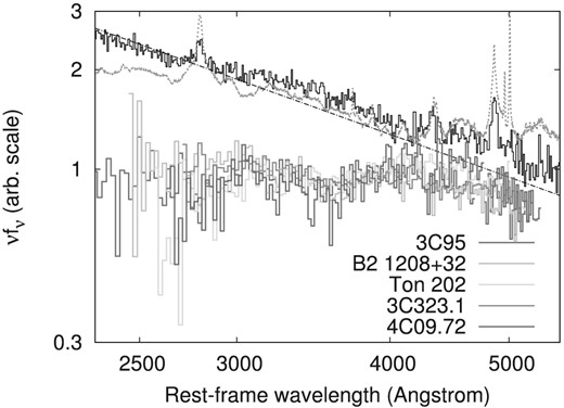
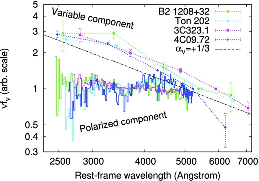
Polarized flux spectra for five quasars showing polarization decrease at λ < 4000 Å (figure 35 of Kishimoto et al. 2004). For comparison, the composite difference spectrum (i.e., the composite variable component spectrum) generated by using two epoch spectra of the SDSS quasars (Ruan et al. 2014) (the black thin solid line), and the composite spectrum of the SDSS quasars (Vanden Berk et al. 2001) (the gray dashed line) are also shown. The dash–dotted line indicates a power-law spectrum with αν = +1/3 (in units of |$f_{\nu }\propto \nu ^{\alpha _{\nu }}$|). (Color online)
List of our target quasars with polarization dip in λ < 4000 Å.*
| Name | Coordinates | E(B − V) | z | P (per cent) | P (per cent) |
|---|---|---|---|---|---|
| RA Dec | at 2891–3600 Å | at 4000–4731 Å | |||
| B2 1208+32 | 12:10:37.56 +31:57:06.02 | 0.017 | 0.388 | 1.01 ± 0.01 | 1.41 ± 0.01 |
| Ton 202 | 14:27:35.60 +26:32:14.55 | 0.019 | 0.366 | 1.25 ± 0.01 | 1.87 ± 0.02 |
| 3C 323.1 | 15:47:43.53 +20:52:16.66 | 0.042 | 0.264 | 1.51 ± 0.01 | 2.19 ± 0.01 |
| 4C 09.72 | 23:11:17.74 +10:08:15.77 | 0.042 | 0.433 | 0.50 ± 0.01 | 0.93 ± 0.01 |
*The redshift z and polarization degree P (per cent) at two rest-frame wavelength ranges are taken from table 6 of Kishimoto et al. (2004). The reported values of P for 4C 09.72 and 3C 323.1 are corrected for the interstellar polarization effect. The Galactic selective extinction E(B − V) based on Schlegel, Finkbeiner, and Davis (1998) is taken from NASA's Extragalactic Database (NED).
1.2 Optical variability in luminous type 1 quasars
Some property other than the polarimetry, optical flux variability, which is an ubiquitous property of AGNs, is also worthy of investigation in connection with the intrinsic spectral shape of the AGN accretion disk spectra. Since the variability amplitude is enormous (typically ∼10%–20%), the variable component in the AGN UV–optical spectra must be reflecting the main energy source of the AGN, namely, the accretion disk emission itself (Gaskell 2008). Moreover, the strong inter-band correlations of the AGN variability indicate that the AGN UV–optical variability is not caused by localized independent fluctuations (having their own temperatures), but is a consequence of some kind of global changes in the accretion disk (Kokubo 2015). Therefore, it is natural to expect that the spectral shape of an AGN accretion disk continuum can be obtained directly as the variable continuum spectral component (Pereyra et al. 2006; Li & Cao 2008; Schmidt et al. 2012; Kokubo et al. 2014; Ruan et al. 2014, and references therein). It should be noted that the BLR emission is less variable than the underlying continuum, known as the intrinsic Baldwin effect (Kinney et al. 1990): Wilhite et al. (2005) showed that the BLR emission lines vary at most 20%–30% as much the continuum emission, and Kokubo et al. (2014) noted that the low ionization lines of Fe ii and Mg ii are even less variable than the high ionization lines. Since the flux contribution from the host galaxy and most of the BLR emission is nonvariable, the spectral shape of the variable component spectra can be derived without suffering from the heavy spectral distortion by these contaminants.
In the NIR wavelength range, several spectral variability studies suggest that the accretion disk spectra revealed as the variable spectral component has a spectral shape as blue as the thermal accretion disk model prediction of αν = 1/3 (Tomita et al. 2006; Lira et al. 2011; Koshida et al. 2014, and references therein). In the near-UV to optical wavelength range, thermal accretion disk models generally predict the spectral turnover to much redder spectral slope (e.g., Kishimoto et al. 2008b). However, Kokubo et al. (2014) examined the spectral variability of ∼9000 Sloan Digital Sky Survey (SDSS) quasars using ∼10 yr multiband light curves available in the SDSS Stripe 82 region, and found that the variable component spectra of quasars are well described by a power-law shape with αν ∼ 1/3 even in the UV–optical wavelength range, and thus are systematically too blue to be explained by the existing thermal accretion disk models even after considering the flux contamination from the (weakly) variable broad emission lines, Fe ii emission lines, and the Balmer continuum emission (see also Schmidt et al. 2012; Ruan et al. 2014, and figure 1). It should also be noted that the strong dip feature at λ < 4000 Å observed in the polarized flux seems to be absent in the composite variable continuum spectra of SDSS quasars (Wilhite et al. 2005; Pereyra et al. 2006; Kokubo et al. 2014; Ruan et al. 2014). In summary, quasar variability studies suggest that the intrinsic accretion disk spectrum revealed as the variable continuum component cannot be explained by existing accretion disk models.
1.3 The goal of this study
As described above, the results from the two kinds of studies seem to be contradicting; on the one hand polarimetric studies suggest that the intrinsic accretion disk spectrum revealed by the spectropolarimetry has a spectral shape consistent with the thermal, optically thick accretion disk model predictions of, e.g., Hubeny et al. (2000), but on the other hand variability studies suggest that the intrinsic accretion disk spectrum obtained as a variable continuum component has too blue a UV spectral shape to be explained by existing accretion disk models. This discrepancy, if confirmed, is a huge problem where the basic assumptions underlying these observations are related to our fundamental understandings of quasar central engine, and thus it definitely offers new insights into the nature of the quasar/AGN BBB emission.
However, we should note that the above statement is currently based on the observations for different quasar samples. Although the quasars in the Kishimoto et al. (2004)'s sample have similar optical spectra as the SDSS quasars (actually B2 1208+32, Ton 202, and 3C 323.1 are contained in the spectroscopically confirmed SDSS quasar catalog; Schneider et al. 2010); on the one hand the variability studies are based on the general population of several thousands of SDSS quasars (e.g., Kokubo et al. 2014), but on the other hand the spectropolarimetric studies are based on the small, and probably biased, sample of quasars (see Schmidt & Smith 2000; this point will be discussed elsewhere).2 The purpose of this work is to examine the optical spectral variability for the quasars showing the Balmer edge-like feature in their polarized flux spectra confirmed by Kishimoto et al. (2004), and probe whether or not these quasars also show flat variable component spectra as the other normal quasars. Here we present the multi-band optical light curves for four out of the five quasars in Kishimoto et al. (2004)'s sample (4C 09.72, B2 1208+32, Ton 202, and 3C 323.1), and compare their spectral shape of the polarized flux and variable flux components.
This paper is organized as follows. In section 2, we present multiband optical light curves of the four quasars obtained by using the 1.05 m Kiso Schmidt telescope at the Kiso Observatory in Japan. Then, we derive the variable component spectra for the quasars from the multi-band light curves by using a “flux gradient method” in section 3. In section 4 we compare the spectral shape of the the variable and polarized component spectra of these quasars in detail (subsection 4.1), and discuss the possible interpretations of the relationship between these two spectral components (subsection 4.2). Finally, our summary and conclusions are given in section 5.
2 Multiband photometric observations with the 1.05 m Kiso Schmidt telescope
We carried out u-, g-, r-, i-, and z-band photometric monitoring observations for four out of the five quasars with polarization dip in λ < 4000 Å in Kishimoto et al. (2004)'s sample (4C 09.72, B2 1208+32, Ton 202, and 3C 323.1; see table 1) from 2015 April to 2016 February, using the 1.05 m Kiso Schmidt telescope being operated by the Kiso Observatory of the University of Tokyo. The 1.05 m Kiso Schmidt telescope is equipped with the Kiso Wide Field Camera (KWFC: Sako et al. 2012), which has eight CCD chips (the field of view is 2| $_{.}^{\circ}$|2 × 2| $_{.}^{\circ}$|2) composed of four CCDs with 2 k × 4 k pixels manufactured by Lincoln Laboratory, Massachusetts Institute of Technology (MIT) and four ST-002A CCDs with 2 k × 4k pixels manufactured by Scientific Imaging Technologies, Inc. (SITe). The average wavelengths of the Kiso/KWFC photometric bands are not precisely known, and thus we assume them to be identical with the SDSS imaging camera, i.e., 3551, 4686, 6166, 7480, and 8932 Å for u, g, r, i, and z bands, respectively, taken from the SDSS website (see also Fukugita et al. 1996; Doi et al. 2010).3 The four target quasars are located within the SDSS Legacy survey footprint (York et al. 2000; Gunn et al. 2006) and thus the photometric calibration can be done by using the SDSS photometry data of the field stars on the same frames with the targets.4
Our observations have been carried out in the queue mode. In the queue mode, calibration data, i.e., dome-flat frames for every filter and bias frames, are usually obtained automatically at the beginning and/or end of each observing night. Since the dark current of the KWFC CCDs is below 5e− [hr−1 pixel−1] at an operational temperature of 168 K (e.g., Sako et al. 2012), we did not obtain dark frames. The five band images were normally obtained quasi-simultaneously in giruz order with four dithering pointings for each band, although the number of the bands and exposures was reduced on several observing nights according to the weather conditions. The exposure time for each image is 30 s for every filter in 2015 April–June, and is 60 s for g, r, and i bands and 120 s for u and z bands in 2015 July–2016 February.
For the observations presented in this paper, we used 2 × 2 binning four MIT chips in FAST readout mode (1|${^{\prime\prime}_{.}}$|88 pixel−1) to reduce the overhead time, and the targets were acquired on to the MIT chip#3 (named as MIT-4 in figure 2 of Sako et al. 2012). Thus, in this work we only reduce and analyse the chip#3 images. The detector temperature is kept at 167.9–168.0 K during the observations. Each of the 2 k × 4 k CCDs of KWFC has a dual amplifier readout. During the data reduction, we treat the two readout areas on chip#3 (upper 1 k × 4 k and lower 1 k × 4 k pixels, corresponding the two amplifiers) separately. During the data reduction, the gain factor and the readout noise of the chip#3 are assumed to be 2.3 electrons per ADU and 15 electrons, respectively, for both of the readout ports. An overscan subtraction for all of the calibration and object frames is carried out by using the column overscan region with the IRAF task colbias.5 The master bias frame for each of the observing nights is generated by median-combining the overscan-subtracted bias frames taken at the same or the closest night, and is used to correct for the large-scale bias pattern. Master dome-flat frames for each of the observing filters are created by median-combining the dome-flat frames taken at the same or the closest night by normalizing the large-scale sensitivity and/or illumination pattern with the use of the IRAF task mkillumflat. These master dome-flat frames are used to correct for the pixel-to-pixel sensitivity variation of the CCD detector. To correct for the global sensitivity inhomogeneity of the detector, we use super sky-flat frames created by median-combining different nights’ object images by masking detected objects using the IRAF task objmasks. During the creation of the master dome-flat and super sky-flat calibration frames, the dead pixel lines at the bottom right-hand portion of chip#3 (X = 1263–2073 and Y = 33–41 pixel coordinates in the 2 × 2 binning mode) are replaced by linear interpolation along columns using the IRAF task fixpix.
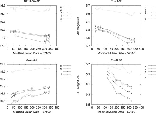
u-, g-, r-, i-, and z-band light curves of B2 1208+32, Ton 202, 3C 323.1, and 4C 09.72, obtained at the Kiso observatory. Galactic extinction is not corrected. (Color online)
Sky background subtraction, source extraction and aperture photometry for the overscan, bias, and pixel-to-pixel and global flat-fielded object frames were carried out using SExtractor (version 2.8.6; Bertin & Arnouts 1996), and coordinate conversion (shifts, pixel scale, and rotation) was carried out using WCSTools imwcs (version 3.8.4; Mink 2006) and USNO-B1.0 catalog (Monet et al. 2003). An automatically interpolated background map is calculated and subtracted from the object frames (namely, we use the SExtractor parameters of BACK_TYPE=AUTO, BACKPHOTO_TYPE=GLOBAL, BACK_SIZE=64, and BACK_FILTERSIZE=6). The dead pixel lines mentioned above are masked during the SExtractor runs. Considering the seeing statistics at the Kiso site (3|${^{\prime\prime}_{.}}$|9 FWHM at median in g band; Morokuma et al. 2014), the extraction aperture is set to 5 pixels (∼9|${^{\prime\prime}_{.}}$|4). The detection and analysis thresholds are set to 3σ, where σ is defined as the sum of the photon noise and the readout noise, not including noises introduced by the overscan/bias subtraction and the flat-fielding processes. It should be noted that the target quasars are observed as pointlike objects, and thus the apparent flux changes due to seeing variations are cancelled by the relative photometry using field stars described below.
The magnitude zero-point shift for each frame was evaluated by taking a 3σ-clipping weighted average of the differences between the instrumental magnitudes and the SDSS model magnitudes [retrieved from the SDSS Data Release 12 (DR12) SkyServer Star view; Alam et al. (2015)] of field stars within the field of view of each of the readout areas on chip#3 (1| $_{.}^{\circ}$|076 × 0| $_{.}^{\circ}$|269). The field stars flagged as CLEAN in the SDSS database were used, and the object frames with no more than 30 position-matched field stars were excluded from the analysis. It is known that the photometric zeropoints of the SDSS magnitude system are slightly offset from those of the AB magnitude system. Thus we apply the recommended offset values of uAB = uSDSS − 0.04 mag, and zAB = zSDSS + 0.02 mag to our calibrated data, following the description on the SDSS website.6 The magnitude to flux conversion is done by assuming the zero magnitude flux as 3631 Jansky (Jy). Since the color-term correction factors for the KWFC SDSS filters have not been determined, in this work we do not apply the color correction. We also decide not to combine the (mostly single-epoch) SDSS Legacy Survey photometric data for the target quasars with our light curves to avoid the possible systematic error due to the noncorrection of the color-term.
The obtained light curves are shown in table 2 and plotted in figure 2. The reported magnitude/flux values for a given filter are the weighted averaged values of the dithering images taken on the same nights. The observation epoch for each data point is expressed in Modified Julian Date (MJD) at the midpoint of the exposures. We confirm that all of the four quasars show flux variability in all five bands during our observations, although the variability amplitude in B2 1208+32 is relatively small compared to the others. The observed variability amplitudes of Δg ∼ 0.1–0.4 mag within ∼200 d in the quasar rest-frame are consistent with the general property of the SDSS quasars (e.g., MacLeod et al. 2012).
KWFC u-, g-, r-, i-, and z-band light curves for B2 1208+32, Ton 202, 3C 323.1, and 4C 09.72.*
| Name | MJD | Magnitude | Error in magnitude | Band |
|---|---|---|---|---|
| B2 1208+32 | 57164.47822 | 16.9528 | 0.0306 | u |
| B2 1208+32 | 57390.64625 | 17.1045 | 0.0167 | u |
| B2 1208+32 | 57402.62973 | 17.0845 | 0.0170 | u |
| B2 1208+32 | 57407.78441 | 17.1105 | 0.0258 | u |
| B2 1208+32 | 57419.86152 | 17.0244 | 0.0291 | u |
*The reported magnitude values are in AB magnitude system, and are not corrected for Galactic extinction. The complete listing of this table is available in the online edition as Supporting Information.
3 Analysis
The flux–flux plots of two-band simultaneous light curves of AGNs and quasars in the UV–optical wavelength range are known to be fitted well with a straight line of y = a + bx, which indicates that the variable continuum component in AGNs and quasars keeps its spectral shape nearly constant over several years to several tens of years of the flux variability (Sakata et al. 2010, 2011; Kokubo et al. 2014; Kokubo 2015; Ramolla et al. 2015 and references therein, although see also Sun et al. 2014). This means that the linear regression slope (gradient) of the flux–flux plot of the quasar two-band light curves can be used as an indicator of the color of the variable component spectrum, since the flux gradient represents the flux ratio of the two-band fluxes of the variable component spectrum (“flux gradient method”: e.g., Choloniewski 1981; Winkler et al. 1992; Hagen-Thorn 1997; Winkler 1997; Glass 2004; Hagen-Thorn 2006; Cackett et al. 2007; Sakata et al. 2010, 2011; Kokubo et al. 2014; Ramolla et al. 2015). The good point of the flux gradient method is that the regression slope is not affected by the flux contamination from the nonvariable spectral components (the host galaxy flux and time-averaged flux level of BLR emission). Thus, applying the flux gradient method to the multi-band light curves, we can derive the relative spectra of the variable component in quasars without suffering from the spectral distortion due to the flux contribution from the nonvariable spectral components (see Kokubo et al. 2014, and references therein). Here we examine the spectral shape of the variable flux component in the four quasars by using the multiband photometric monitoring data obtained at the Kiso observatory. The two-band simultaneous light curve for each target and for each band-pair is generated by combining the two-band measurements taken on the same nights.
Figure 3 shows the flux–flux plots of the light curves of B2 1208+32, Ton 202, 3C 323.1, and 4C 09.72, overplotted with the best-fitting linear regression line for each band-pair derived by using the MPFITEXY IDL routine (Williams et al. 2010). The MPFITEXY routine depends on the MPFIT package (Markwardt 2009), and is able to cope with the data with an intrinsic scatter, which is automatically adjusted to ensure χ2/(degrees of freedom) ∼1 (see Tremaine et al. 2002; Novak et al. 2006; Park et al. 2012 for details). Flux values in figure 3 are corrected for the Galactic extinction (Galactic extinction values for the SDSS filters are taken from NED; Schlegel et al. 1998). For B2 1208+32, Ton 202, and 3C 323.1, we choose to use the i-band flux as a reference of the continuum flux variability and as an x-axis in the flux–flux plots (i.e., independent variable), since the i-band wavelength range is less contaminated by broad emission lines than the other bands. For 4C 09.72, whose observed-frame i-band wavelength range contains the Hβ line, the r-band flux is instead used as a reference of the continuum flux variability and as the x-axis in the flux–flux plots.
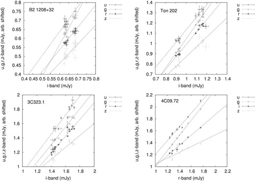
Galactic-extinction-corrected flux–flux plots of the light curves of B2 1208+32, Ton 202, 3C 323.1, and 4C 09.72 obtained at the Kiso observatory. The flux values are arbitrarily shifted on the y-axis for clarity. (Color online)
The best-fitting linear regression parameters (regression slope and intercept) for the flux–flux plots are summarized in table 3. Since the variability amplitude of B2 1208+32 is small and the sampling of the light curves is poor, the regression parameters are not well constrained for B2 1208+32, especially in the i–u band-pair. For the other quasars, the flux–flux plots are well fitted with linear regression lines. We should also note that the regression intercepts of i–u, i–g, i–r, r–u, and r–g band-pairs (where the y-axis represents shorter wavelengths) are generally negative, and conversely those of i–z, r–i, and r–z band-pairs (where the y-axis represents longer wavelengths) are positive. This means that the total observed flux spectra of these quasars become bluer when they get brighter (“bluer when brighter” trend), which is a common feature observed in the light curves of the SDSS quasars (see Kokubo et al. 2014 for details).
Best-fitting linear regression parameters (slope and intercept) for the two-band flux–flux plots.*
| Name | Band-pair | Slope | Intercept |
|---|---|---|---|
| (x–y) | [mJy] | ||
| B2 1208+32 | i–u | 1.371 ± 0.395 | −0.284 ± 0.251 |
| B2 1208+32 | i–g | 1.814 ± 0.186 | −0.523 ± 0.121 |
| B2 1208+32 | i–r | 1.241 ± 0.126 | −0.158 ± 0.081 |
| B2 1208+32 | i–z | 1.061 ± 0.288 | +0.425 ± 0.187 |
| Ton 202 | i–u | 1.222 ± 0.068 | −0.220 ± 0.068 |
| Ton 202 | i–g | 1.421 ± 0.040 | −0.376 ± 0.041 |
| Ton 202 | i–r | 1.210 ± 0.038 | −0.172 ± 0.039 |
| Ton 202 | i–z | 0.955 ± 0.079 | +0.716 ± 0.082 |
| 3C 323.1 | i–u | 1.331 ± 0.169 | −0.611 ± 0.272 |
| 3C 323.1 | i–g | 1.250 ± 0.082 | −0.544 ± 0.127 |
| 3C 323.1 | i–r | 1.166 ± 0.051 | −0.292 ± 0.079 |
| 3C 323.1 | i–z | 0.830 ± 0.102 | +1.241 ± 0.160 |
| 4C 09.72 | r–u | 1.148 ± 0.076 | −0.244 ± 0.108 |
| 4C 09.72 | r–g | 1.269 ± 0.029 | −0.156 ± 0.042 |
| 4C 09.72 | r–i | 0.857 ± 0.044 | +0.304 ± 0.063 |
| 4C 09.72 | r–z | 0.485 ± 0.151 | +1.160 ± 0.216 |
*The reported uncertainty is ± 1σ.
Figure 4 shows the relative variable component spectra of the four quasars derived from the linear regression slopes of the flux–flux plots (table 3), along with the polarized component spectra taken from Kishimoto et al. (2004). Figure 5 shows all of these spectra simultaneously to emphasize the similarity of the spectral shape of the variable component spectra among the target quasars. In figures 4 and 5, the uncertainty of the variable component spectra in the reference band (r band for B2 1208+32, Ton 202, and 3C 323.1, and i band for 4C 09.72) is taken to be zero. Detailed comparisons of the spectral shape of the variable component spectra and the polarized component spectra and a discussion about them are given in the next section.
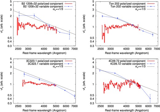
Comparison of the spectral shape of the variable and polarized components in the optical spectra of B2 1208+32, Ton 202, 3C 323.1, and 4C 09.72. Dotted lines indicate the variable component spectra derived in this work (see section 3), and the solid lines are the polarized component spectra taken from Kishimoto et al. (2004). The polarized component spectra are the same as figure 1. The two spectra in each panel are scaled to match each other approximately at the red side of the polarized component spectrum. For comparison, a power-law spectrum with αν = +1/3 (in units of |$f_{\nu }\propto \nu ^{\alpha _{\nu }}$|) is also shown.
Same as in figure 4, but all objects are shown simultaneously. The variable component spectra are scaled to 1 in the i band for clarity. The spectra of B2 1208+32, Ton 202, 3C 323.1, and 4C 09.72 are colored green, cyan, magenta, and blue, respectively.
4 Discussion
4.1 Notes on the effect of the BLR emission variability
In figures 4 and 5, it is clearly seen that the variable component spectra of the four quasars have a very blue power-law-like spectral shape throughout the rest-frame near-UV to optical spectra region, which is as blue as the long-wavelength limit value of the thermal accretion disk prediction αν = 1/3, in good agreement with the previous works on the AGN and quasar variability (e.g., Collier et al. 1999; Kokubo et al. 2014; Ruan et al. 2014; Fausnaugh et al. 2016; MacLeod et al. 2016; see subsection 1.2). This means that the variable component spectra are significantly bluer than the polarized component spectra (and thus than the thermal accretion disk model predictions) in the near-UV spectral region of the four quasars. Figure 4 shows that the discrepancy of the spectral shape between the variable and polarized components (if these spectra are scaled to the same flux level at optical wavelengths) results in an about twofold discrepancy in the emitted energy at UV wavelengths. As discussed in subsection 1.3, this huge discrepancy strongly suggests that there are fundamental problems in our current understanding of the quasar UV–optical variability and/or polarization; namely, that one (or both) of the two interpretations—one states that the polarized component spectrum should represent the intrinsic accretion disk continuum spectrum (e.g., Kishimoto et al. 2004, 2008b), the other states that the variable component spectrum represents it well (e.g., Pereyra et al. 2006; Schmidt et al. 2012; Kokubo et al. 2014; Ruan et al. 2014)—is (are) wrong.
It should first be noted that, as mentioned in subsection 1.2, broad-band photometric light curves containing the rest-frame spectral regions of the broad emission lines are unavoidably (more or less) affected by the contamination from the broad line flux variability, although the continuum variability is often larger than the broad line variability at least by a factor of a few (intrinsic Baldwin effect; e.g., Kinney et al. 1990; Wilhite et al. 2005; Bian et al. 2012; Kokubo et al. 2014). The variable component spectra in figure 4 actually show small deviations from single power-law spectra, which can possibly be attributed to the flux variability of BLR emission: the z band of Ton 202 and B2 1208+32 contains the Hα line, the i band of 4C 09.72 and the r band of Ton 202 and 3C 323.1 contain the Hβ
line, and the g band contains blends of higher order Balmer lines and the Balmer continuum emission from the BLR, all of which are known to show flux variability as a result of reverberation of the ionizing continuum emission (e.g., Maoz et al. 1993; Korista & Goad 2001, 2004; Kokubo et al. 2014; Edelson et al. 2015; Fausnaugh et al. 2016, and references therein). The dominant BLR emission in u band is Fe ii pseudo-continuum and Mg ii emission, but several spectral variability studies show that the variability of these low-ionization emission lines is very weak and does not significantly contribute to the variable spectral component (see Goad et al. 1999; Kokubo et al. 2014; Modzelewska et al. 2014; Sun et al. 2015, and references therein). In any case, it is very difficult to attribute the twofold flux excess in the near-UV region (u and g bands in the observed frame) of the variable component spectra compared to the polarized component spectra (seen in figure 4) to the variable BLR emission contamination, considering the huge energy required to fill the gap.
More direct observational evidence against the non-accretion disk variable component contamination in the near-UV region is the observed strong inter-band. The flux–flux plots in figure 3, especially for 4C 09.72, show a very strong linear correlation. Such a strong inter-band correlation is generally observed in AGNs and quasars (Sakata et al. 2010; Kokubo 2015), and validates the use of the flux gradient method described in section 3. Since the BLR is located at a few tens or hundreds of light-days (note that our observation period is ∼200 d in the quasar rest-frame) away from the inner region of the accretion disk in luminous quasars like those analysed in this work (according to the well-established BLR radius–optical luminosity relation; e.g., Bentz et al. 2013), the observed strong inter-band correlation suggests that the huge flux contribution from the BLR emission is unlikely and that there exists essentially a single dominant variable continuum component throughout the near-UV to optical wavelengths.
One may think that this power-law-like variable component spectra seen in figures 4 and 5 are from the variable optical synchrotron emission. However, if it was true, the optical polarized component spectra would be dominated by the intrinsically polarized synchrotron emission and thus have the same spectral shape as those of the variable component spectra. A similarity between the variability amplitude and the spectral shape of the variable component observed in the four quasars that have general properties of the SDSS quasars, which are mostly radio-quiet quasars (e.g., Ivezić et al. 2002), also suggests that the variable component in these luminous type 1 quasars are related to the accretion disk emission rather than the optical synchrotron emission. Inversely, it seems to be difficult to explain the observed complex spectral shape of the polarized flux spectra by the optical synchrotron emission contribution (see Kishimoto et al. 2003, 2004 for more detailed discussion).
4.2 Possible interpretations of the relationship between variable and polarized spectral components
Because there seems to be no explanation for the large flux deficit in the near-UV region seen in the polarized component spectra of the quasars (compared to the variable component spectra), we may have to consider that the UV–optical polarization in the luminous type 1 quasars cannot solely be explained by the Thomson (electron) scattering, and there may be some unknown (de)polarization mechanisms producing the observed decrease of the polarization degree in the near-UV wavelengths, considering that the variable flux component spectra should represent the spectral shape of intrinsic accretion disk emission.
On the other hand, it could also be possible that the blue spectral shape of the variable component is not representing the shape of the total flux spectrum coming from the whole surface of the quasar accretion disk. Generally speaking, a causal argument suggests that the short-term (several days to several tens of days) flux variability observed in AGNs and quasars is caused at the disk radii smaller than several tens of light-days from the central black hole (e.g., Starling et al. 2004; Sun et al. 2014). On the basis of this causal argument and the observational fact of the strong linear inter-band flux–flux correlation of the quasar variability on all time-scales (see e.g., Sakata et al. 2010), it seems to be natural to consider that the quasar UV to optical flux variability is always caused by temperature fluctuations within a certain disk radius, which must result in a variable component spectrum that is bluer than the total flux spectrum from the disk. The construction of quantitative models based on the idea described above and comparison with observations are beyond the scope of this work, and these will be discussed in a subsequent paper.
Finally, it should also be noted that, although quantitative comparisons with model spectra are currently impossible, there is still room to consider that the observed polarization properties in the four quasars with a λ < 4000 Å polarization dip may be explained by the intrinsic polarization imprinted on the accretion disk atmosphere. By referring to the model calculations of Laor, Netzer, and Piran (1990) (see also Shields et al. 1998; Hsu & Blaes 1998; Koratkar & Blaes 1999), Kishimoto et al. (2003) and Antonucci et al. (2004) stated that, in a certain accretion disk model parameter space, even though the total flux (and thus the variable component) of the accretion disk spectrum has no feature around the Balmer edge spectral region, the polarization degree (and thus the polarized component) spectrum can show the decreasing feature blueward of the Balmer edge due to the increase of the absorption opacity.7 If this is true, our result of the discrepancy of the spectral shape between the variable component and polarized component in the four quasars can be explained so that the variable component spectrum is a scaled copy of the featureless accretion disk continuum; on the other hand, the polarized component spectrum only represents the intrinsically polarized accretion disk continuum component.
Although above we have listed several implications of the discrepancy between the variable component and polarized component spectra in quasars, it is definitely impossible to conclusively decide whether the polarized component or the variable component spectrum represents the intrinsic accretion disk spectrum well, or if both of the interpretations are invalid, with the currently available data. The only way to probe the true nature of the relationship between the variable component and the polarized component in the quasar spectra is the examination of the polarimetric variability, which has rarely been investigated for AGNs and quasars (see e.g., Merkulova & Shakhovskoy 2006; Gaskell et al. 2012; Afanasiev et al. 2015). For example, Kishimoto, Antonucci, and Blaes (2003) noted that Ton 202 showed evidence of slight changes of the polarization degree at λ < 4000 Å dip region within a year time-scale. This may indicate the presence of the fast-moving absorption material responsible for the Balmer-edge feature in the edge-on trajectory between the inner accretion disk region and the scatterer (e.g., Jiang et al. 2016), which must be confirmed by further spectropolarimetric follow-up observations. Future intensive photometric and/or spectroscopic polarimetric monitoring observations will clarify the causes of the discrepancy between the spectral shapes of the polarized component and variable component in luminous type 1 nonblazar quasars.
5 Summary and conclusions
In the literature, it is suggested that the UV–optical polarized flux spectra of the luminous type 1 quasars are representing the intrinsic spectral shape of the quasar accretion disk emission, and several quasars are showing Balmer edge features (specifically, decrease of the polarized flux at λ < 4000 Å) in their polarized flux spectra which can be interpreted as the imprint of the opacity effect on the accretion disk atmosphere (e.g., Kishimoto et al. 2003; Antonucci et al. 2004; Kishimoto et al. 2004, 2008b; Hu & Zhang 2012). On the other hand, it is also assumed in several previous works that the UV–optical variable component spectra of quasars are a good indicator of the intrinsic spectral shape of the quasar accretion disk emission (e.g., Pereyra et al. 2006; Schmidt et al. 2012; Kokubo et al. 2014; Ruan et al. 2014). In this work, we examined the consistency of the above-mentioned assumptions through the investigation of whether the variable component spectra have the same spectral shape as the polarized flux component spectra in a sample of four λ < 4000 Å polarization-decreasing quasars spectropolarimetrically confirmed by Kishimoto et al. (2004) (4C 09.72, 3C 323.1, Ton 202, and B2 1208+32). The result is negative, where the variable component spectra are significantly bluer compared to the polarized flux component spectra, especially in the near-UV spectral region: the variable component spectra of these quasars are confirmed to be well represented by a single power-law component with αν ∼ 1/3 through the rest-frame UV–optical wavelength range, resulting in the twofold excess of the emitted energy at UV wavelengths compared to the polarized flux spectra. Although it is impossible to decide which of the two assumptions are invalid (or if both are) only from the currently available observational constraints, we can at least say that this discrepancy in the spectral shape implies either (1) the decrease of polarization degree in the rest-frame UV wavelengths does not indicate the Balmer absorption edge feature but is induced by some unknown (de)polarization mechanisms, or (2) the UV–optical flux variability is occurring preferentially at the hot inner radii of the accretion disk and thus the variable component spectra do not reflect the whole accretion disk emission. Future photometric and/or spectroscopic polarimetric monitoring observations will be useful for clarifying the causes of this discrepancy between the spectral shapes of the polarized component and the variable component, and consequently the true nature of the accretion disk emission in the luminous type 1 nonblazar quasars.
We thank Yuki Sarugaku for his support during the KWFC queue mode observations. We are grateful to all the staff in the Kiso Observatory for their efforts to maintain the observation system. We thank the referee, Makoto Kishimoto, for carefully reading our manuscript and for giving useful comments. This work was supported by JSPS KAKENHI Grant Number 15J10324.
This research has made use of NASA's Astrophysics Data System Bibliographic Services. This research has made use of the NASA/IPAC Extragalactic Database (NED), which is operated by the Jet Propulsion Laboratory, California Institute of Technology, under contract with the National Aeronautics and Space Administration. Funding for SDSS-III has been provided by the Alfred P. Sloan Foundation, the Participating Institutions, the National Science Foundation, and the U.S. Department of Energy Office of Science. The SDSS-III web site is http://www.sdss3.org/. SDSS-III is managed by the Astrophysical Research Consortium for the Participating Institutions of the SDSS-III Collaboration including the University of Arizona, the Brazilian Participation Group, Brookhaven National Laboratory, Carnegie Mellon University, University of Florida, the French Participation Group, the German Participation Group, Harvard University, the Instituto de Astrofisica de Canarias, the Michigan State/Notre Dame/JINA Participation Group, Johns Hopkins University, Lawrence Berkeley National Laboratory, Max Planck Institute for Astrophysics, Max Planck Institute for Extraterrestrial Physics, New Mexico State University, New York University, Ohio State University, Pennsylvania State University, University of Portsmouth, Princeton University, the Spanish Participation Group, The University of Tokyo, University of Utah, Vanderbilt University, University of Virginia, University of Washington, and Yale University.
Supporting Information
Additional Supporting Information may be found in the online version of this article.
Table 2.
The quasars discussed in this work are not in the SDSS Stripe 82 region and do not have multi-band light curves. Moreover, the SDSS does not provide multiepoch spectral data for these quasars.
Although we have also been observing the other quasar 3C 95 since 2015 September, we do not include it in the sample of this work because it is not in the SDSS Legacy survey footprint; thus currently the absolute flux calibration cannot be performed. Further observations on this object and the construction of the reference star catalog around it are in progress and will be reported elsewhere.
IRAF is distributed by the National Optical Astronomy Observatory, which is operated by the Association of Universities for Research in Astronomy (AURA) under a cooperative agreement with the National Science Foundation.
Although these models are generally claimed to suffer from the wrong polarization direction (i.e., a polarization direction perpendicular to the disk's rotation axis, contrary to the observations), it is also suggested that absorption opacity effects can in some cases change the polarization position angle to the direction parallel to the disk's rotation axis (Nagirner effect; e.g., Gnedin & Silantev 1978; Matt et al. 1993; Agol et al. 1998).
References
