


Abstract
Average hard-tail X-ray emission in the soft state of nine bright Atoll low-mass X-ray binaries containing a neutron star (NS-LMXBs) are investigated by using the light curves of MAXI/GSC (Gas Slit Camera) and Swift/BAT (Burst Alert Telescope). Two sources (4U 1820−30 and 4U 1735−44) exhibit a large hardness ratio (15–50 keV/2–10 keV: HR >0.1), while the other sources distribute at HR ≲ 0.1. In either case, HR does not depend on the 2–10 keV luminosity. Therefore the difference of HR is due to the 15–50 keV luminosity, which is Comptonized emission. The Compton cloud is assumed to be around the neutron star. The size of the Compton cloud would affect the value of HR. Although the magnetic field of an NS-LMXB is weak, we could expect a larger Alfvén radius than the innermost stable circular orbit or the neutron star radius in some sources. In such cases, the accretion inflow is stopped at the Alfvén radius and would create a relatively large Compton cloud. This would result in the observed larger Comptonized emission. By attributing the difference of the size of Compton cloud to the Alfvén radius, we can estimate the magnetic fields of neutron stars. The obtained lower/upper limits are consistent with the previous results.
1 Introduction
A neutron-star low-mass X-ray binary (NS-LMXB) consists of a weakly magnetized neutron star and a low-mass star. NS-LMXBs are known to exhibit soft and hard states in the X-ray band when their mass-accretion rates are high and low, respectively (e.g., Mitsuda et al. 1989; Matsuoka & Asai 2013). In the soft state, the spectra are dominated by a soft/thermal component, while a hard/Comptonized component is also recognized. The soft/thermal component is well described by an optically thick standard accretion disk model (Shakura & Sunyaev 1973). If the magnetic field of the NS is weak (≤108 G), the magnetic field does not affect the accretion flow, and the accretion disk can extend down to the NS surface. Most of the gas in the disk accretes on to the NS equatorial region. As the luminosity decreases, a soft-to-hard transition occurs in the inner disk from optically thick to thin. Then the radius of the inner disk becomes larger. It is called a truncated disk (Done et al. 2007). The luminosity of the soft-to-hard transition is known to be 1%–4% of the Eddington luminosity (Maccarone 2003). In the hard state, the spectra are dominated by a hard/Comptonized component, while a soft/thermal component is still required. The geometry of the accretion flow changes to the optically thin disk and then the flow accretes to the whole surface of the NS.
The hard/Comptonized component has been observed in both soft and hard states (see Barret 2001 for a review). However, there are differences between the two states in the fitting parameters (the oprital depth and the electron temperature) with the Comptonized component. In the soft state, the optical depth (τ) and the electron temperature (kTe) of the Comptonized component are τ ∼ 5–15 and kTe = a few keV, while those in the hard state are τ ∼ 2–3 and kTe = a few tens of keV. There are two possible locations for the Compton cloud. One is that the formation of a Compton cloud takes place in a transition layer (TL: Titarchuk et al. 1998) located between the disk and NS (e.g., Seifina & Titarchuk 2012; Titarchuk et al. 2013). The other possible location is an accretion disk corona (ADC) above the disk (e.g., Church et al. 2014). Both the location of the Compton cloud and the origin of the seed photons remain uncertain. Furthermore, an additional hard X-ray component has been detected above ∼30 keV in both states (e.g., Paizis et al. 2006). The origin of the emission also remains uncertain, although there are several models, such as Comptonization by bulk motion of accreting matter near the NS (e.g., Paizis et al. 2006), Comptonization by non-thermal electrons accelerated in a jet (e.g., Di Salvo et al. 2006), and synchrotron emission of energetic electrons (e.g., Markoff et al. 2001). Titarchuk, Seifina, and Shrader (2014) reported that the additional hard X-ray component was evidence for the presence of a hot outer part to the TL (see also Seifina et al. 2015).
NS-LMXBs have been classified into two groups, Z sources and Atoll sources, based on their behavior on the color–color diagram and the hardness–intensity diagram (Hasinger & van der Klis 1989). Z sources are bright and sometimes reach close to the Eddington luminosity. On the other hand, Atoll sources are less bright, and some of them exhibit hard/soft spectral state transitions. In the color–color diagram, the distribution can be divided into two main regions, “banana” and “island”. The spectrum is usually softer in the banana than in the island. The distributions of the diagrams (of color–color and hardness–intensity) depend on the energy band, the instrument response, and the absorbing column density towards the source (Done & Gierliński 2003; Kuulkers et al. 1994). Gladstone, Done, and Gierliński (2007) investigated how the banana branch moves in the color–color diagram (soft color: 4–6.4 keV/3–4 keV; hard color: 9.7–16 keV/6.4–9.7 keV) for inclination angles of 30°, 60°, and 70°. The change is mainly in the soft color. They also investigated the effect of kTe of 2.5, 3.0, and 3.5 keV for each inclination angle. This matches very well with the location and the shape of the banana branches in their color–color diagrams.
The surface magnetic field of the NS is believed to be higher in the Z sources (∼109 G) than in the Atoll sources (∼108 G) (Zhang & Kojima 2006). For example, the magnetic field of the Z-source Cyg X-2 was estimated to be 2.2 × 10⁹ G from the observed oscillations in the horizontal branch and the beat frequency model (Focke 1996). For the transient Z-source XTE J1701−462, the magnetic field was estimated to be ∼(1–3) × 109 G from the interaction between the magnetosphere and the radiation-pressure-dominated accretion disk (Ding et al. 2011). Meanwhile, two Atoll sources, 4U 1608−52 and Aql X-1, were estimated to have magnetic fields of 107–108 G from the propeller effect (4U 1608−52: Chen et al. 2006; Asai et al. 2013, Aql X-1: Campana et al. 1998; Zhang et al. 1998; Asai et al. 2013). However, Titarchuk, Bradshaw, and Wood (2001) suggested that both Z sources and Atoll sources have a very low surface magnetic fields of ∼107–108 G based on their magneto-acoustic wave model and the observed kHz quasi-periodic oscillations (QPOs). Also using the kHz QPO, Campana (2000) estimated the magnetic field of ∼(1–8) × 108 G for Cyg X-2 from the kHz QPO observability in the variations of the NS magnetosphere radius (Alfvén radius). Campana (2000) also reported that the magnetic fields of two Atoll sources, 4U 1820−30 and Aql X-1, were estimated to be ∼2 × 10⁸ G and ∼(0.3–1) × 108 G, respectively.
In general, the effect of the magnetic fields of NS-LMXBs is ignored because it is weak. However, in some cases, the importance of the effect is suggested (e.g., Campana 2000; Cui et al. 1998; Ding et al. 2011; Wang et al. 2011). Ding et al. (2011) suggested that the inner disk radius could be set by the magnetospheric radius when the gas pressure from the disk decreases by large radiation pressure and the magnetosphere expands. Wang et al. (2011) considered a TL between the innermost Keplerian orbit and the magnetosphere, and suggested that the accretion flow is disturbed by several instabilities. Furthermore, Campana (2000) suggested that the disappearance of the kHz QPO was related to the disappearance of the magnetosphere (see also Cui et al. 1998). They also noted that the effect of the magnetic field of an NS must be taken into account. In this study, we considered the effect of the magnetic field of an NS.
We investigated the average hardness ratio (hereafter HR: 15–50 keV/2–10 keV) in the soft state of nine bright Atoll NS-LMXBs using MAXI (Matsuoka et al. 2009)/GSC (Gas Slit Camera: Mihara et al. 2011; Sugizaki et al. 2011)1 and Swift (Gehrels et al. 2004)/BAT (Burst Alert Telescope: Barthelmy et al. 2005)2 from 2009 August 15 (MJD = 55058) to 2015 August 15 (MJD = 57249). In section 2, we describe the data selection and analysis of the hardness–luminosity diagram. In section 3, we discuss the relation between hard tail emission and magnetic fields of NS-LMXB. The conclusion is presented in section 4.
2 Analysis and results
2.1 Distribution of hardness ratio (15–50 keV/2–10 keV)
We obtained long-term one-day bin light curves of MAXI/GSC and Swift/BAT for nine bright Atoll NS-LMXBs. The light curves of the 2–10 keV band of GSC, the 15–50 keV band of BAT, and the HR of the two bands are shown for each source in figures 1 –3. The obtained count rates of GSC and BAT were converted to luminosities by assuming a Crab-like spectrum (Kirsch et al. 2005) and the distances listed in table 1. The assumption of a Crab-like spectrum is acceptable in the hard state, because the energy spectrum is dominated by the Comptonized emission approximated by a power law with a photon index of 1–2. On the other hand, in the soft state, the energy spectrum is dominated by the thermal emission. The luminosity obtained by assuming Crab-like spectrum is underestimated in the 2–10 keV band, but is overestimated in the 15–50 keV band. As a result, the HR of two energy bands is overestimated by 2.0 times (see Asai et al. 2015 for detail). Therefore, we handle only the relative difference (see the Appendix).
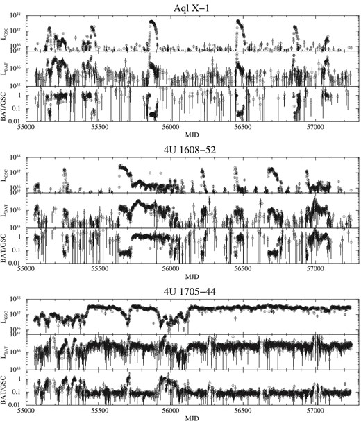
One-day GSC light curves in the 2–10 keV band, one-day BAT light curves in the 15–50 keV band, and the hardness ratio (BAT/GSC) of Aql X-1, 4U 1608−52, and 4U 1705−44. LGSC and LBAT are the luminosities in units of erg s−1. Vertical error bars represent 1 σ statistical uncertainty.
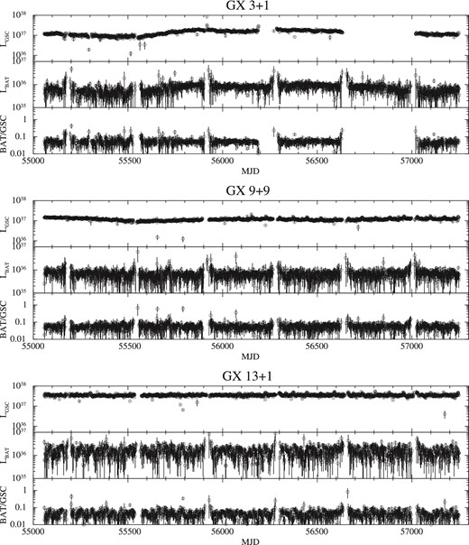
Same as figure 1, but for GX 3+1, GX 9+9, and GX 13+1. One-year periodic rises before and after data gaps in the Swift/BAT light curves are due to instrumental effect. MAXI/GSC data gaps in GX 3+1 in MJD = 56187–56287 and 56652–56997 are due to contamination source.
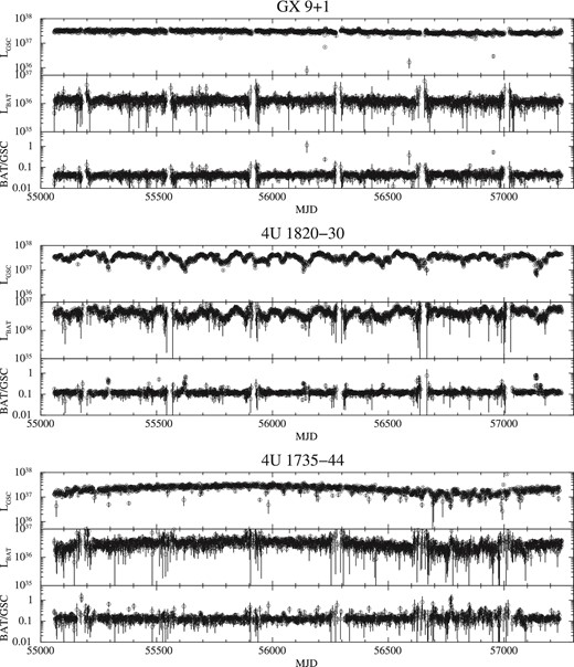
Same as figure 1, but for GX 9+1, 4U 1820−30, and 4U 1735−44.
Periods of the soft states defined by MAXI/GSC and Swift/BAT, and distance used in this paper.
| Name | Period of soft states (MJD) | Distance (kpc) | Ref.* |
|---|---|---|---|
| Aql X-1 | 55157–55170, 55451–55479, 55857–55899, 56460–56513, 56853–56873 | 5 | (1) |
| 4U1608−52 | 55260–55272, 55645–55721, 56213–56226, 56442–56445, 56673–56734, 56937–56945 | 4.1 | (2) |
| 4U1705−44 | 55410–55684, 55717–55915, 56048–57249 | 7.4 | (1) |
| GX 3+1 | 55058–57249 | 4.5 | (4) |
| GX 9+9 | 55058–57249 | 5 | (3) |
| GX 13+1 | 55058–57249 | 7 | (1) |
| GX 9+1 | 55058–57249 | 5 | (1) |
| 4U 1820−30 | 55058–55288, 55306–55615, 55629–56130, 56141–56474, 56482–56619, 56681–56986, | 7.6 | (1) |
| 56995–57132, 57145–57151, 57167–57249 | |||
| 4U 1735−44 | 55058–56766, 56775–57249 | 8.5 | (2) |
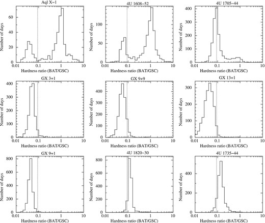
Figure 4 shows the histograms (number of days) of the HR (BAT/GSC) of all nine NS-LMXBs. The peak around HR = 1 corresponds to the hard state, while the distribution around HR = 0.1 corresponds to the soft state. The soft state shows two peaks. The boundary of the two peaks (HR at the smallest value) is 0.09 (dotted line in figure 4). We also show the distributions of HRs for the individual sources in figure 5. The distributions of the soft state are divided into two groups using the peak value of HR. One group has a peak HR smaller than 0.09: Aql X-1, 4U 1608−52, GX 3+1, GX 9+9, GX 13+1, and GX 9+1. The other has a peak HR larger than 0.09: 4U 1820−30 and 4U 1735−44. We note that 4U 1705−44 is exceptional since the peak is at HR = 0.09.
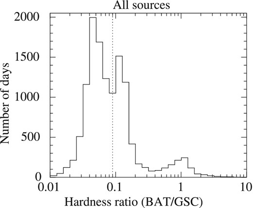
Distributions of hardness ratios of BAT/GSC for all nine NS-LMXBs. The distributions were constructed from data with a significance >1 σ. The vertical dotted line represents the threshold between two soft states (see text for explanation).
Distributions of hardness ratios of BAT/GSC for nine NS-LMXBs. The vertical dotted lines represent the threshold that we determined in figure 4.
2.2 Hardness–luminosity diagram
To investigate the difference between two groups in the soft state, we selected the data of only the soft state. Table 1 shows periods of the soft state that are analyzed in this paper. Four sources (GX 3+1, GX 9+9, GX 13+1, and GX 9+1) stayed in the soft state during the observed period, which is obvious since there is no distribution of the hard state (around HR = 1) in figure 5. In contrast to these four sources, the other five sources show both the soft and hard states. The individual selection of the soft state is summarized as follows.
Aql X-1: The source stayed in the soft state during five outbursts (see figure 1). The HR threshold between the soft and hard states was chosen as 0.222 in one-day bin data, which is taken after the analysis in Asai et al. (2015). When the state transition continued for more than one day, we excluded the data and used the data only in a stable HR.
4U 1608−52: The source stayed in the soft state during six outbursts and mini-outbursts during MJD = 55900–56100 (see figure 1). The HR threshold was chosen as 0.224 in one-day bin data after Asai et al. (2015). We excluded the data during the transition in the same way as for Aql X-1. We also removed the data of mini-outbursts, because the spectral states repeated between the soft and hard states in short durations (less than several tens of days).
4U 1705−44: The source stays in soft state during three outbursts and mini-outbursts during MJD = 55058–55400 and 55800–56100 (see figure 1). The HR threshold was chosen as 0.355 in one-day bin data after Asai et al. (2015). We excluded the data during the transition in the same way as Aql X-1, and the data of mini-outbursts as 4U 1608−52.
4U 1820−30: Although 4U 1820−30 stays in the soft states for most of the time, it changed to the hard state (HR>0.2: Asai et al. 2015) eight times (see figure 3). We excluded the data in the eight hard states.
4U 1735−44: 4U 1735−44 stays in the soft states most of the time, and it changed to the hard state (HR ∼1) only once (see figure 3). We excluded the data in the hard state.
Figure 6 shows hardness–luminosity diagrams during the soft state for each source. The gray backdrop is the distribution of all the nine sources. The vertical dotted lines represent the threshold that we determined in figure 4. The nine sources are divided into two groups except for 4U 1705−44. One is distributed in the part below the threshold of 0.09 (Aql X-1, 4U 1608−52, GX 3+1, GX 9+9, GX 13+1, and GX 9+1.). The other is distributed in the part higher than the threshold (4U 1820−30 and 4U 1735−44).
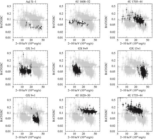
Hardness–luminosity diagram, which plotted against a backdrop of all nine NS-LMXBs. The data are 5-d averaged. The distributions are constructed from data with a significance >3 σ. The horizontal dotted lines represented the the threshold that we determined in figure 4.
After excluding 4U 1705−44, both figure 5 and figure 6 show that eight NS-LMXBs are divided into two groups by the threshold of HR = 0.09. This result is consistent with the results of spectral model fitting for RXTE data of 4U 1820−30 and GX 3+1 (see the Appendix). In the next section, we discuss the difference of HR.
3 Discussion
We investigated average hard-tail X-ray emission in the soft state of nine bright Atoll NS-LMXBs, where the magnitude of the hard tail is defined by HR (15–50/2–10 keV, see figures 4 and 5). We can classify the HR into at least two groups: the larger hard tail (4U 1820−30 and 4U 1735−44) and the smaller hard tail (Aql X-1, 4U 1608−52,GX 3+1, GX 9+9, GX 13+1, and GX 9+1) (see figures 6 and 10). In this section, we give a reasonable phenomenological interpretation of the observational results. The results would be related to properties of each NS, such as magnetic fields.
3.1 Differences of inclination, electron temperature, and seed photon
The difference of HR (15–50/2–10 keV) comes from that of the 15–50 keV luminosity, because the HR is almost constant for a wide range of the 2–10 keV luminosity. For example, the 2–10 keV luminosities of both sources, Aql X-1 and 4U 1820−30, are in the same range of (∼1.2–30) × 1036 erg s−1. On the other hand, the HR of Aql X-1 is smaller than 0.09 and that of 4U 1820−30 is larger than 0.09, as shown in figure 6. The emission in the 15–50 keV energy band is known to originate from the Comptonized component.
We show how the HR of the energy range (15–50/2–10 keV) would not be affected by the following differences below.
Inclination. In general, the difference in the HR distribution is interpreted via the difference of the inclination of the system (Gladstone et al. 2007). When the inclination is high, the HR tends to be large because of the large τ. GX 13+1 is known to be a high inclination system because of the periodic dipping and the deep Fe absorption features (60°–80°; Díaz Trigo et al. 2012; D'Aì et al. 2014). If the distribution of HR in figure 6 reflects the inclination, the HR distribution of GX 13+1 is expected to be in the part that is higher than the threshold (0.09). However, the result is the opposite. The other sources would not be high inclination systems because periodic dipping has not been reported. Thus the value of HR would be independent of the inclination when we used the energy band of 15–50/2–10 keV.
Electron temperature kTe of Compton cloud. In the soft state, kTe is typically a few keV (see Barret 2001 for a review). The difference in the HR distribution is interpreted by the difference of kTe of the Compton cloud (Gladstone et al. 2007). When kTe is high, HR tends to be large because Compton up-scattering occurs up to high energy. Titarchuk, Seifina, and Frontera (2013) reported that kTe changes from 2.9 to 6 keV for upper banana in both 4U 1820−30 and GX 3+1. If the distribution of HR in figure 6 reflected kTe, the distributions of HR in both 4U 1820−30 and GX 3+1 are expected to be the same. However, the distributions of the two sources are not the same and are divided above and below the threshold (0.09). The change of kTe as described by Titarchuk, Seifina, and Frontera (2013) would appear as scatter in the HR for each source.
The HR of 4U 1820−30 and 4U 1735−44 is larger than the threshold. In the case of 4U 1820−30, the composition of the accreting matter is helium (Rappaport et al. 1987). kTe would be higher than the hydrogen accretion of other sources. However, the orbital period (and thus separation) of 4U 1735−44 is large and the companion star would be a normal star. Thus the accreting matter would be hydrogen. Helium accretion cannot be a common reason for the large Compton component. Thus, the classification of two groups of HR is independent of kTe.
Origin of the seed photon to Compton cloud. The Comptonized component is also characterized by the seed photon. The seed photons are considered to be soft photons from an NS surface and/or disk photons in soft state (e.g., Sakurai et al. 2012; Seifina & Titarchuk 2012; Titarchuk et al. 2013). The difference would not affect the distribution of HR, because the HR is almost constant over the large range of luminosity of (7–50)× 1036 erg s−1.
Therefore, we propose that the difference between the two groups would be due to the size of the Compton cloud.3 The group with HR larger than 0.09 (4U 1820−30 and 4U 1735−44) would have larger Compton cloud than the other group with HR smaller than 0.09. We notice that the HR of 4U 1705−44 indicates an intermediate value between two groups.
3.2 Location of Compton cloud
In the soft state, Comptonized emission is considered to be formed in the TL located between the accretion disk and NS surface (e.g., Seifina & Titarchuk 2012; Titarchuk et al. 2013) and/or in the ADC above the accretion disk (e.g., Church et al. 2014). Although the location is controversial, the size of the Compton cloud would change with the amount of accretion flow. However, there is no correlation between the observed luminosity and the HR between the two groups. Here, let us take into account of the magnetic field of the NS. Although the magnetic field of an NS in an NS-LMXB is considered to be weak, in some cases the effect of the magnetic field is taken into account (e.g., Campana 2000; Cui et al. 1998; Ding et al. 2011; Wang et al. 2011). In the soft state, most of the gas in the disk accretes on to the NS equatorial region, because the disk can extend to the NS surface or the innermost stable circular orbit (ISCO). The accretion flow is thermalized on the NS surface, and the emission from there is Comptonized by the plasma around the NS. However, if the magnetic field of the NS is ≥108 G, the Alfvén radius would be larger than the ISCO/NS surface. In this case, the accretion disk would be terminated at the Alfvén radius. A similar situation is suggested by Ding et al. (2011), although they considered the radiation-pressure-dominated accretion disk. Then the accretion flow spreading vertically at the Alfvén radius would create relatively large Compton cloud. In the TL model, the outer boundary of the TL corresponds to the Alfvén radius. The difference between HRs is dependent on whether the Alfvén radius is larger than the ISCO/NS surface.
We calculated RA as a function of L when B is from 0.5 × 10⁸ G to 3.5 × 10⁸ G, as shown in figure 7. We adopted η = 0.52 because the accretion flow is considered to be a disk-like accretion flow in the soft state. We also adopted MNS = 1.4 M⊙ and RNS = 106 cm. We also plotted the radius of the ISCO and the NS. The ISCO is 3rg, where rg is the Schwarzschild radius (= 2GM/c2). Here, the ISCO is 1.2 × 106 cm for MNS = 1.4 M⊙. When L is 1037 erg s−1, RA is larger than the ISCO for B > 1.5 × 10⁸ G. In this case, the accretion flow would be stopped and spread at the Alfvén radius, and then the relatively large Compton cloud would be created. As a result, the HR would be large (for example HR > 0.09). On the other hand, when B < 1 × 10⁸ G, the RA is smaller than both the ISCO and the NS surface. In this case, the accretion flow is not affected by the magnetic field, and then most of the gas in the disk accretes on to the NS equatorial region. The HR would be low (for example HR < 0.09).
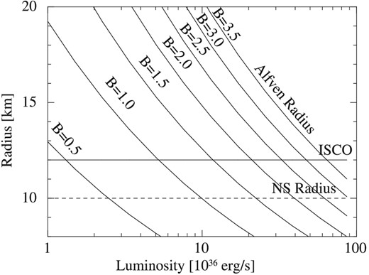
Alfvén radius (RA) as a function of luminosity, where B is from 0.5 × 10⁸ G to 3.5 × 10⁸ G.
Figure 8 illustrates the schematic drawings of suggested geometry of an NS-LMXB in a soft state. Assuming MNS = 1.4 M⊙ and B = 2 × 10⁸ G, (a) RA = 1.2 × 106 cm, (b) RA = 1.3 × 106 cm, and (c) RA = 1.5 × 106 cm for L = 20 × 1036 erg s−1, 15 × 1036 erg s−1, and 10 × 1036 erg s−1, respectively. When the luminosity increases, RA becomes smaller and the size of Compton cloud would be smaller. However, the solid angle from the photon source is constant. Thus, HR is constant even if the luminosity is increasing, as long as RA is larger than the ISCO [(b) and (c) in the lower panel].
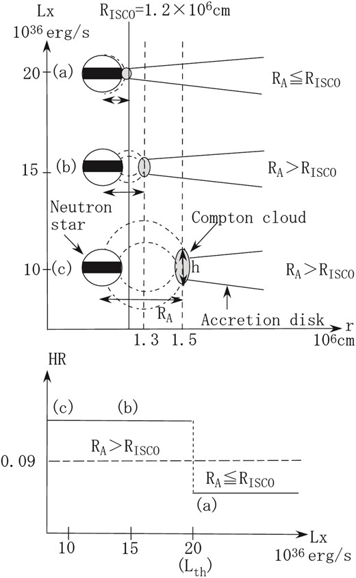
Schematic drawings of suggested geometry of NS-LMXB in the soft state. Assuming MNS = 1.4 M⊙ and B = 2 × 10⁸ G, (a) RA = 1.2 × 106 cm, (b) RA = 1.3 × 106 cm, and (c) RA = 1.5 × 106 cm corresponding to L = 20 × 1036, 15 × 1036, and 10 × 1036 erg s−1, respectively. The HR representing the solid angle of the Compton cloud changed between (a) and (b), while it stays constant in (b) and (c).
Here, we define the threshold luminosity (Lth) where RA equals the ISCO in equation (1). In the lower panel, Lth = 20 × 1036 erg s−1. When the luminosity is higher than Lth, RA is smaller than the ISCO and HR is below 0.09 (a). On the other hand, when the luminosity is lower than Lth, RA is larger than ISCO and HR is above 0.09 [(b) and (c)].
3.3 Magnetic field derived from the threshold luminosity
Next, we try to estimate the magnetic field (B) of the NS using the difference in HR. We defined Lth in the previous subsection. Here, we use the ISCO rather than the NS surface, since the ISCO is 1.2 × 106 cm, which is larger than RNS, employing traditional values of RNS = 1 × 106 cm and MNS = 1.4 M⊙. We note that the ISCO is not always larger than RNS (e.g., Wang et al. 2015). Since uncertainty remains for both the radius and mass, we adopt the traditional values. If the luminosity is higher than Lth, RA is smaller than the ISCO. In this case, the accretion disk would not be affected by the magnetic field and the large Compton cloud would not be created. The HR remains small (<0.09). When the observed HR is always smaller than 0.09 in one source, the minimum observed luminosity becomes the upper limit of Lth. On the other hand, when the observed HR is always larger than 0.09, the maximum observed luminosity becomes the lower limit of Lth. Thus, we can estimate the upper/lower limits of B from the upper/lower limits of Lth.
First, we determined Lth from the hardness–luminosity diagrams (figure 6). The values of Lth are listed in table 2. Here, for 4U 1705−44, we adopted the lower-end luminosity of the distribution on HR = 0.09 as Lth, because the HR of 4U 1705−44 is distributed around HR = 0.09. This means that the luminosity changes over Lth. Substituting RA = ISCO of 1.2 × 106 cm and L = Lth in equation (1), we obtained B as in table 2. The values B of Aql X-1 and 4U 1608−52 are consistent with those reported previously. Although the B of 4U 1820−30 (>3.2 × 10⁸ G) is somewhat larger than the reported value of ∼2 × 10⁸ G (Campana 2000), our values are consistent in the sense that the B of 4U 1820−30 is larger than those of Aql X-1 and 4U 1608−52.
Threshold luminosity and corresponding magnetic fields.
| Name | HR of peak | L th* | B | kHz QPO† | Reported B | References‡ |
|---|---|---|---|---|---|---|
| (1036 erg s−1) | (108 G) | (108 G) | ||||
| Aql X-1 | <0.09 | ≲ 11 | ≲ 1.4 | ○ | 0.3–1.9 | (1), (2), (3), (4) |
| 4U 1608−52 | <0.09 | ≲ 8 | ≲ 1.2 | ○ | 0.5–1.6 | (4), (5) |
| 4U 1705−44 | = 0.09 | ≲ 20 | ≲ 1.9 | ○ | — | — |
| GX 3+1 | <0.09 | ≲ 8 | ≲ 1.2 | — | — | — |
| GX 9+9 | <0.09 | ≲ 9 | ≲ 1.3 | — | — | — |
| GX 13+1 | <0.09 | ≲ 30 | ≲ 2.4 | — | — | — |
| GX 9+1 | <0.09 | ≲ 23 | ≲ 2.1 | — | — | — |
| 4U 1820−30 | >0.09 | ≳ 55 | ≳ 3.2 | • | ∼2 | (3) |
| 4U 1735−44 | >0.09 | ≳ 34 | ≳ 2.5 | • | — | — |
*Threshold luminosity in the 2–10 keV band (see text for explanation).
†• : kHz QPOs have been reported in soft state. ○ : kHz QPOs have been reported, although the state is not clear. — : Not reported (van der Klis 2006).
Next, we plot the hardness–“normalized luminosity” diagram for all the sources in figure 9b. The luminosities of figure 6 were normalized by the Lth. Figure 9a shows the hardness–luminosity diagram for all the sources to realize the effect of the normalization. After the normalization, in figure 9b, the data points are distributed on a single trend from upper-left to lower-right. The data points in the upper-left section can be interpreted to mean that the accretion flow is spread vertically at RA. Meanwhile, the data points in the lower-right section can be interpreted to mean that the accretion flow is unaffected by the magnetic fields. We also presented the hardness–“normalized luminosity” diagrams for individual sources in figure 10.
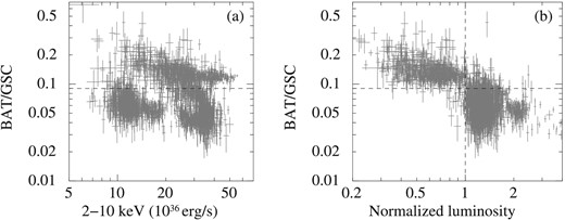

According to the fact that the frequency of the upper kHz QPO is related to the Keplerian frequency at the inner edge of an accretion disk, Campana (2000) suggested that the disappearance of kHz QPO at high luminosities may be related to the disappearance of the magnetosphere at the time when RA reaches RNS. Then we can assume that the disappearance of the kHz QPO is related to a smaller HR (<0.09) in our sources. In table 2 we listed an existence of reported kHz QPO (van der Klis 2006). The kHz QPO was observed from large HR (≥0.09) sources (4U 1705−44, 4U 1820−30, and 4U 1735−44) while it was not observed from small HR (≤0.09) sources (GX 3+1, GX 9+9, GX 13+1, and GX 9+1). In the cases of Aql X-1 and 4U 1608−52, the kHz QPO was detected even though they have small HR. For Aql X-1, Campana (2000) reported that the kHz QPO disappeared at the luminosity (2–10 keV) higher than 3.6 × 1036 erg s−1. Similarly, for 4U 1608−52, the kHz QPOs were detected only when the luminosity (2–20 keV) dropped down to 1037 erg s−1 (Méndez et al. 1998). Namely, the kHz QPO was not detected in the soft state (>1037 erg s−1). Therefore, the existence/absence of the kHz QPO is consistent with our results of the large/small HR.
4 Conclusion
We investigated average hard-tail X-ray emission in the soft state of nine bright Atoll NS-LMXBs by using the light curves of MAXI/GSC and Swift/BAT, and tried to relate the difference of HR values to that of B of NSs. When RA is larger than the ISCO, the accretion disk would be stopped and spread at RA, and then the relatively large Compton cloud would be created. Then, the HR would become large (>0.09), and the observed luminosity is lower than Lth, where Lth is the luminosity at which RA equals the ISCO. We can derive the lower limit of B of the NS from the lower limits of Lth. Since the HR of 4U 1820−30 and 4U 1735−44 is large, Bs is estimated as B ≳ 2.5 × 10⁸ G. The upper limit of B is given for the other seven sources. These results are consistent with the previous results.
We would like to acknowledge the MAXI team for MAXI operation and for analyzing real-time data.
Appendix. Hardness–intensity diagram
Here we investigate the validity of assuming a Crab-like spectrum for a soft state in the conversion from the count rate of GSC and BAT to the luminosity (see subsection 2.1). In a soft state, the luminosity obtained in this way is underestimated in the 2–10 keV, but is overestimated in the 15–50 keV. Therefore, we handle only the relative difference of HR. Here we compare HR obtained by assuming a Crab-like spectrum with that obtained by spectral model fitting for RXTE (Rossi X-ray Timing Explorer) data. The latter was taken from table 4 of Titarchuk, Seifina, and Frontera (2013) for 4U 1820−30 and table 4 of Seifina and Titarchuk (2012) for GX 3+1. Figure 11 shows the hardness–luminosity diagram in both cases. The data of 4U 1820−30 included those of the soft and hard state in both cases. The energy band of HR is slightly different. The HR in figure 11a is 15–50 keV/2–10 keV. In figure 11b, the HR of 4U 1820−30 and GX 3+1 is 10–50 keV/3–10 keV and 10–60 keV/3–10 keV, respectively. In spite of the difference of energy band, the HR of 4U 1820−30 is larger than that of GX 3+1 in both figures 11a and 11b. Thus, the relative difference of HR assuming a Crab-like spectrum is consistent with the result of spectral model fitting.
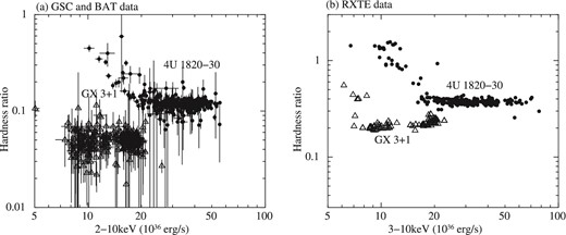
Hardness–luminosity diagram of 4U 1820−30 and GX 3+1. The data of 4U 1820−30 included the data of both soft and hard state. (a) The data are obtained by GSC and BAT. The 2–10 keV luminosities are obtained by assuming Crab-like spectrum. The HR is 15–50 keV/2–10 keV. The data are 5-d averaged. (b) The data are obtained by RXTE, which is listed in table 4 of Titarchuk, Seifina, and Frontera (2013) for 4U 1820−30 and table 4 of Seifina and Titarchuk (2012) for GX 3+1. The HR of 4U 1820−30 and GX 3+1 is 10–50 keV/3–10 keV and 10–60 keV/3–10 keV, respectively.
Correctly speaking, the “size” is the optical depth × the solid angle from the photon source of the Compton cloud. If the optical depth is similar, the difference of the solid angle is reflected. When the distance between the photon source and the Compton cloud is similar, the solid angle is proportional to the size of the Compton cloud. We use the word “size” in this context.
We notice that Wang (1997) estimated η ∼ 1 even in the case of disk-like accretion flow. They calculated torque in an inclined magnetic moment axis to the spin axis assuming that the spin axis was normal to the disk plane.
References
