


Abstract
While narrow absorption lines (NALs) are relatively stable, broad absorption lines (BALs) and mini-BAL systems usually show violent time variability within a few years via a mechanism that is not yet understood. In this study, we examine the variable ionization state (VIS) scenario as a plausible mechanism, as previously suspected. Over three years, we performed photometric monitoring observations of four mini-BAL and five NAL quasars at zem ∼ 2.0–3.1 using the 105 cm Kiso Schmidt Telescope in u, g, and i bands. We also performed spectroscopic monitoring observation of one of our mini-BAL quasars (HS 1603+3820) using the 188 cm Okayama Telescope over the same period as the photometric observations. Our main results are as follows: (1) Structure function (SF) analysis revealed that the quasar UV flux variability over three years was not large enough to support the VIS scenario, unless the ionization condition of outflow gas is very low. (2) There was no crucial difference between the SFs of mini-BAL and NAL quasars. (3) The variability of the mini-BAL and quasar light curves was weakly synchronized with a small time delay for HS 1603+3820. These results suggest that the VIS scenario may need additional mechanisms such as variable shielding by X-ray warm absorbers.
1 Introduction
Quasars are useful background sources when investigating objects along our lines of sight. The absorption features in quasar spectra (i.e., quasar absorption lines; QALs) are usually classified into intervening QALs, which originate in intervening galaxies and the intergalactic medium, and intrinsic QALs, whose origin is physically associated with background quasars. The latter comprise the accelerated gas outflow from the quasars themselves.
The gas outflow can be accelerated by several possible mechanisms: radiation pressure in the lines and continuum (Murray et al. 1995; Proga et al. 2000), magnetocentrifugal force (Everett 2005), and thermal pressure (Chelouche & Netzer 2005). However, the primary mechanism of the gas outflow is poorly understood. The outflow winds are important, because (1) they eject angular momentum from the quasar accretion disk and promote accretion of new gas (Murray et al. 1995; Proga et al. 2000); (2) they expel large amounts of energy and metallicity, thus contributing to the chemical evolution of the local universe (Moll et al. 2007; Di Matteo et al. 2005); and (3) they regulate star formation in nearby interstellar and intergalactic regions.
Broad absorption lines (BALs), defined as lines with a full width at half maximum (FWHM) exceeding 2000 km s−1 (Weymann et al. 1991), have been routinely used in outflow wind studies. However, the line parameters (e.g., column density and line width) of BALs cannot be measured by model fitting because the line profiles are hopelessly blended and saturated. On the other hand, mini-BALs (with FWHMs of 500–2000 km s−1) and narrow absorption lines (NALs; with FWHMs ≤ 500 km s−1) contain internal structures that can be model-fitted to probe their properties (e.g., Misawa et al. 2005, 2007b). The observed BALs, mini-BALs, or NALs depend on the viewing angle to the outflow stream (Murray et al. 1995; Ganguly et al. 2001). The detection rates of BALs, mini-BALs, and NALs are ∼10%–15%, ∼5%, and ∼50%, respectively (Hamann et al. 2012), which probably indicates the global covering fraction of the absorbers around the continuum sources.
Around 70%–90% of BALs are time-variable within 10 years (Gibson et al. 2008; Capellupo et al. 2011, 2012, 2013). As an extreme case, the measured C iv BAL variability of SDSS J141007.74+541203.3 is only 1.20 d in the quasar rest frame (Grier et al. 2015), representing the shortest timescale of absorption line variability ever reported. Recently, Misawa, Charlton, and Eracleous (2014) monitored the spectra of mini-BAL and NAL quasars, and found that only the former show significant time variability in their absorption lines.
However, the physical mechanisms of the absorption line variability remain unclear. To date, three scenarios have been proposed: (1) gas clouds crossing our line of sight (the gas motion scenario), (2) variable attenuation by flux that is redirected toward our line of sight by scattering material around the quasar (the reflection scenario), and (3) changing ionization levels in the outflow gas [the variable ionization state (VIS) scenario].
Misawa et al. (2005, 2007b) spectroscopically monitored the C iv mini-BAL in the quasar HS 1603+3820 for more than four years. They found multiple troughs in the mini-BAL that vary in concert. This finding eliminates the gas motion scenario (at least in 1603+3820) because it implies simultaneous crossing of gas clouds over our line of sight, which is unlikely. Misawa et al. (2010) also rejected the reflection scenario, because in spectropolarimetric observations of the same mini-BAL system, the fraction of polarized flux (i.e., the flux redirected by scattering material) is only ∼0.6%, too small to support the reflection scenario. Gibson et al. (2008) found no correlations between quasars and absorption line variability in 13 BAL quasars. On the other hand, Trévese et al. (2013) simultaneously monitored the equivalent widths (EWs) of BALs and the ultraviolet (UV) luminosities of their host quasars (i.e., ionizing photon density) and found clear correlations in a single quasar, supporting the VIS scenario. The VIS scenario has not been tested in mini-BAL/NAL quasars and is still being debated.
In this study, we verify the VIS scenario in the light curves of four mini-BAL quasars and five NAL quasars (hereafter, quasar variability).1 We also search for possible correlations between the outflow and quasar parameters, as discussed in the literature [e.g., Giveon et al. 1999 (G99, hereafter); Vanden Berk et al. 2004 (VB04, hereafter); de Vries et al. 2005; Wold et al. 2007; Wilhite et al. 2008 (W08, hereafter); Meusinger & Weiss 2013]. Section 2 of this paper describes the sample selection, observation, and data analysis. In section 3, we present the photometric data of mini-BAL/NAL quasars. Section 4 discusses the viability of the VIS scenario in mini-BAL and NAL quasars and the possible correlations between parameters. Results are summarized in section 5. Throughout, we adopt a cosmological model with H0 = 70 km s−1 Mpc−1, Ωm = 0.27, and ΩΛ = 0.73.
2 Observation and data analysis
2.1 Sample selection
Our samples are selected based on the availability of multi-epoch high dispersion spectroscopic studies in Misawa, Charlton, and Eracleous (2014). We sampled four mini-BAL quasars (HS 1603+3820, Q 1157+014, Q 2343+125, and UM 675) and five NAL quasars (Q 0450−13102 Q 0940−1050, Q 1009+2956, Q 1700+6416, and Q 1946+7658), whose absorption line variabilities (or non-variabilities) have been already studied by Misawa, Charlton, and Eracleous (2014) using Subaru with the High Dispersion Spectrograph (HDS; R ∼ 450000), Keck with the High Resolution Echelle Spectrometer (HIRES; R ∼ 360000), and Very Large Telescope (VLT) with the Ultraviolet and Visual Echelle Spectrograph (UVES; R ∼ 40000) in time intervals of ∼4–12 yr. Our sample quasars are summarized in table 1.
2.2 Imaging observations
Photometric observations were performed by the 105 cm Kiso Schmidt Telescope with a Kiso Wide Field Camera (KWFC: Sako et al. 2012). The eight 2 K × 4 K charge-coupled devices (CCDs) in the KWFC provide a field of view (FoV) of 2| $_{.}^{\circ}$|2 × 2| $_{.}^{\circ}$|2. Since five of our nine quasars are located in the Sloan digital sky survey (SDSS) field, our photometry used the SDSS (u, g, and i) filters instead of the Johnson filters. Moreover, as the u band is less sensitive than the g and i bands, we adopted a 2 × 2 binning mode (1|${^{\prime\prime}_{.}}$|89 pixel−1) for the u-band observations.
The quasars were repeatedly observed from 2012 April 14 to 2014 October 16 with a typical monitoring interval of three months, representing the typical variability timescale of BALs (e.g., Capellupo et al. 2011, 2012, 2013). Observation logs of the individual quasars are summarized in table 2. The log excludes Q 0450−1310 and Q 1946+7658 in the u band, because the continuum fluxes of these quasars are heavily absorbed by the foreground intergalactic medium (i.e., the Lyα forest). Bias subtraction, flat-fielding, sky subtraction, and world coordinate system matching were performed by an automatic analysis pipeline. The same pipeline was used for supernova discoveries in the Kiso Supernova Survey (KISS) project (Morokuma et al. 2014).
2.3 Relative photometry
The extraction and magnitude measurements of quasars and comparison stars were performed by SExtractor (Bertin & Arnouts 1996). Regions crowded with stars were selected by the flux estimation code FLUX_BEST.
Since we mainly investigate the light curves of quasars (i.e., the relative magnitudes between observing epochs), we do not need to measure their true magnitudes. Therefore, we performed relative photometry by simultaneously monitoring the quasars and effective photometric standard stars (hereafter called comparison stars) near the quasars. The comparison stars were selected as follows. We chose two (unsaturated) bright stars near the target quasars in the same CCDs and investigated their relative magnitudes Δm (=|ms1 − ms2|), where ms1 and ms2 are the magnitudes of the bright stars. If the relative variability between the two stars |Δm −〈Δm〉|, where 〈Δm〉 is the average value of all observations, was always below 0.05 mag and below the 3 σ level of the photometric errors (i.e., Δm was very stable), one of the stars was designated a comparison star. Otherwise, we continued searching for stars that satisfied the above criteria. A single comparison star was used in all epochs, unless different stars in different filters were required.
In equation (2), σij2 is the sum of squares of the photometric error in the comparison star between epochs i and j.
2.4 Properties of sample quasars
Sample quasars.
| Quasar | RA* | Dec† | m V (MV)‡ | z em § | z abs ‖ | v ej ♯ | Variability** | |$\langle {\rm EW}_{\rm abs, C\,{\small {I}V}} \rangle {}^{\dagger \dagger}$| | 〈ΔEW〉‡‡ | (ΔEW)max§§ | R ‖‖ | log Lbol♯♯ | log MBH/M*** | 円† | Ref.‡‡‡ |
|---|---|---|---|---|---|---|---|---|---|---|---|---|---|---|---|
| (mag) | (km s−1) | (Å) | |||||||||||||
| mini-BAL quasar | |||||||||||||||
| HS 1603+3820 | 16:04:55.4 | +38:12:01 | 15.99 (−30.60) | 2.542 | ∼2.43 | ∼9500 | Y | 13.10 | 2.03 ± 0.38 | 7.83 ± 2.16 | <0.2 | 48.27 | 9.72 | 2.87 | 1,5,8 |
| Q 1157+014 | 11:59:44.8 | +01:12:07 | 17.52 (−28.49) | 2.00 | ∼1.97 | ∼3000 | Y§§§ | 37.96 | 1.09 ± 1.21 | 1.41 ± 1.61 | 471 | 47.47 | 9.14 | 1.70 | 2,5,2 |
| Q 2343+125 | 23:46:28.2 | +12:49:00 | 17.0 (−29.62) | 2.515 | ∼2.24 | ∼24400 | N | 2.48 | 0.84 ± 0.48 | 1.25 ± 0.82 | 1.27 | 47.87 | 9.08 | 4.90 | 11,5,9 |
| UM 675 | 01:52:27.3 | −20:01:06 | 17.4 (−28.81) | 2.15 | ∼2.13 | ∼1900 | Y | 4.51 | –‖‖‖ | 1.54 ± 0.32 | 438 | 47.58 | 9.52 | 0.91 | 3,5,10 |
| NAL quasar | |||||||||||||||
| Q 0450−1310 | 04:53:13.6 | −13:05:55 | 16.5 (−29.89) | 2.300 | 2.2307 | 37037 | N | – | – | – | <1.69 | 48.01 | 9.59 | 1.90 | 4,12,12 |
| Q 0940−1050 | 09:42:53.4 | −11:04:25 | 16.90 (−30.26) | 3.080 | 2.8347 | 18578 | N | 1.64 | 0.03 ± 0.04 | 0.04 ± 0.06 | <2.58 | 48.11 | 9.48 | 3.59 | 4,12,12 |
| Q 1009+2956 | 10:11:56.6 | +29:41:41 | 16.05 (−30.71) | 2.644 | 2.2533 | 33879 | N | 1.73 | –‖‖‖ | 0.01 ± 0.07 | <1.58 | 48.49 | 9.53 | 7.21 | 4,6,8 |
| Q 1700+6416 | 17:01:00.6 | +64:12:09 | 16.17 (−30.66) | 2.722 | 2.7125 | 767 | N | 0.30 | 0.02 ± 0.01 | 0.03 ± 0.02 | <1.24 | 48.98 | 10.4 | 3.02 | 4,6,2 |
| Q 1946+7658 | 19:44:55.0 | +77:05:52 | 16.20 (−30.94) | 3.051 | 2.8928 | 927 | N | 0.29 | –♯♯♯ | –♯♯♯ | <1.35 | 48.38 | 10.23 | 1.12 | 4,7,7 |
*Right ascension.
†Declination.
‡ V-band magnitude (Vega) from Véron-Cetty and Véron (2010). Values in parentheses are absolute magnitudes.
§C iv emission redshift.
‖Apparent redshift of C iv outflow.
♯Ejection velocity determined from the quasar emission redshift (in km s −1).
**Absorption line variability (Yes or No). See Misawa, Charlton, and Eracleous (2014).
††Averaged equivalent width of C iv absorption line given by the outflows (in Å), from Misawa, Charlton, and Eracleous (2014).
‡‡Averaged amplitude of C iv absorption variabilities, from Misawa, Charlton, and Eracleous (2014).
§§ Maximum amplitude of C iv absorption variabilities, from Misawa, Charlton, and Eracleous (2014).
‖‖Radio loudness.
♯♯Bolometric luminosity.
***Central black hole mass (in units of solar units).
†††Eddington ratio, Lbol/LEdd.
‡‡‡References for R, log Lbol, and log MBH in numerical order: (1) Just et al. (2007), (2) Shen et al. (2011), (3) Griffith et al. (1994), (4) Misawa et al. (2007a), (5) Misawa, Charlton, and Eracleous (2014), (6) Wu et al. (2010), (7) Kuhn et al. (1995), Różańska et al. (2014), (9) Trainor and Steidel (2012), (10) Dietrich et al. (2009), (11) FIRST survey, and (12) this paper.
§§§Variability is seen only in Si iv mini-BAL with a significance level of ∼2.4 σ (Misawa et al. 2014).
‖‖‖Cannot be calculated because our sample was limited to two epochs.
♯♯♯We cannot calculate these because C iv NAL was observed only once (Misawa et al. 2014).
Log of observations.
| QSO | Obs. date | Band | Δtrest* | t EXP † |
|---|---|---|---|---|
| (d) | (s) | |||
| HS 1603+3820 (mini-BAL QSO) | 2012 Apr 14 | u | 0 | 180 × 5 |
| 2012 Apr 14 | g | 0 | 60 × 5 | |
| 2012 Apr 14 | i | 0 | 60 × 5 | |
| 2012 May 12 | i | 7.9 | 60 × 5 | |
| 2012 May 12 | g | 8.2 | 60 × 5 | |
| 2012 May 13 | u | 8.2 | 300 × 5 | |
| 2012 Aug 24 | u | 37.3 | 300 × 5 | |
| 2012 Aug 24 | g | 37.3 | 60 × 3 | |
| 2012 Sep 21 | g | 45.2 | 180 × 3 | |
| 2013 Jan 15 | g | 77.9 | 180 × 5 | |
| 2013 Feb 6 | g | 84.1 | 60 × 5 | |
| 2013 Feb 7 | i | 84.4 | 300 × 3 | |
| 2013 Mar 4 | u | 91.5 | 300 × 3 | |
| 2013 May 17 | g | 112.4 | 60 × 5 | |
| 2013 May 17 | i | 112.4 | 60 × 5 | |
| 2013 May 18 | u | 112.6 | 420 × 1, 480 × 3, 600 × 1 | |
| 2013 Sep 27 | g | 149.9 | 120 × 5 | |
| 2013 Sep 27 | i | 149.9 | 120 × 5 | |
| 2013 Sep 29 | u | 150.5 | 300 × 5 | |
| 2014 May 19 | g | 215.0 | 60 × 5 | |
| 2014 May 21 | u | 216.5 | 300 × 4 | |
| 2014 Sep 2 | g | 245.9 | 120 × 2, 180 × 2, 240 × 1 | |
| Q 1157+014 (mini-BAL QSO) | 2012 Apr 14 | u | 0 | 300 × 5 |
| 2012 Apr 14 | g | 0 | 120 × 5 | |
| 2012 Apr 14 | i | 0 | 60 × 1, 120 × 4 | |
| 2012 May 12 | u | 9.3 | 300 × 5 | |
| 2012 May 12 | g | 9.3 | 120 × 5 | |
| 2012 May 12 | i | 9.3 | 120 × 5 | |
| 2013 Jan 15 | g | 92 | 180 × 1, 300 × 5 | |
| 2013 Feb 6 | g | 99.3 | 180 × 5 | |
| 2013 Mar 3 | g | 107.7 | 180 × 5 | |
| 2013 Mar 3 | i | 107.7 | 180 × 3 | |
| 2013 Mar 4 | u | 108.0 | 600 × 3 | |
| 2013 May 17 | g | 132.7 | 120 × 5 | |
| 2013 May 17 | i | 132.7 | 120 × 5 | |
| 2013 Dec 10 | u | 201.7 | 600 × 4 | |
| 2013 Dec 10 | g | 201.7 | 360 × 3 | |
| 2013 Dec 10 | i | 201.7 | 180 × 5 | |
| 2014 May 19 | g | 255.0 | 120 × 5 | |
| Q 2343+125 (mini-BAL QSO) | 2012 Aug 25 | g | 0 | 120 × 1, 180 × 1, 240 × 1 |
| 2012 Sep 8 | g | 4.0 | 120 × 5 | |
| 2012 Oct 21 | g | 16.2 | 120 × 5 | |
| 2012 Oct 21 | i | 0 | 120 × 5 | |
| 2012 Nov 16 | g | 23.6 | 120 × 4 | |
| 2012 Nov 16 | i | 7.4 | 120 × 5 | |
| 2013 Sep 27 | g | 113.2 | 120 × 4, 240 × 1 | |
| 2013 Sep 27 | i | 97.0 | 120 × 5 | |
| 2013 Sep 28 | u | 0 | 300 × 5 | |
| 2014 Sep 2 | g | 209.9 | 120 × 1, 180 × 4 | |
| 2014 Oct 16 | u | 109.0 | 300 × 1, 360 × 4 | |
| 2014 Oct 16 | g | 222.5 | 120 × 5 | |
| 2014 Oct 16 | i | 206.2 | 120 × 4 | |
| UM 675 (mini-BAL QSO) | 2012 Aug 26 | g | 0 | 300 × 2 |
| 2012 Sep 8 | g | 4.1 | 120 × 5 | |
| 2012 Oct 21 | g | 17.8 | 120 × 5 | |
| 2012 Oct 21 | i | 0 | 120 × 5 | |
| 2012 Nov 17 | g | 26.0 | 120 × 4 | |
| 2012 Nov 18 | i | 8.9 | 120 × 5 | |
| 2013 Sep 27 | g | 126.0 | 180 × 1, 240 × 3 | |
| 2013 Sep 28 | u | 0 | 420 × 5 | |
| 2013 Sep 28 | i | 108.6 | 120 × 5 | |
| 2014 Sep 2 | g | 234.0 | 180 × 3 | |
| 2014 Oct 16 | u | 121.6 | 300 × 2 | |
| 2014 Oct 16 | i | 230.2 | 120 × 4 | |
| Q 0450−1310 (NAL QSO) | 2012 Sep 9 | g | 0 | 60 × 2, 120 × 3 |
| 2012 Oct 20 | g | 12.4 | 60 × 3, 120 × 2 | |
| 2012 Oct 20 | i | 0 | 120 × 5 | |
| 2012 Nov 17 | g | 20.9 | 180 × 3 | |
| 2012 Nov 18 | i | 8.8 | 60 × 5 | |
| 2013 Feb 6 | g | 45.4 | 180 × 2, 240 × 1 | |
| 2013 Sep 27 | g | 116.0 | 120 × 5 | |
| 2013 Sep 27 | i | 103.6 | 60 × 5 | |
| 2013 Dec 10 | g | 138.5 | 240 × 5 | |
| 2013 Dec 10 | i | 126.1 | 60 × 5 | |
| Q 0940−1050 (NAL QSO) | 2012 Apr 14 | u | 0 | 300 × 5 |
| 2012 Apr 14 | i | 0 | 60 × 5 | |
| 2012 May 11 | g | 0 | 60 × 5 | |
| 2012 May 12 | i | 6.9 | 60 × 5 | |
| 2012 May 13 | u | 7.1 | 300 × 3 | |
| 2012 Nov 17 | g | 46.6 | 300 × 4, 240 × 1 | |
| 2013 Jan 15 | g | 61.0 | 180 × 5 | |
| 2013 Feb 6 | g | 66.4 | 180 × 5 | |
| 2013 Mar 3 | g | 72.5 | 120 × 5 | |
| 2013 Mar 4 | u | 79.4 | 600 × 2 | |
| 2013 May 17 | g | 90.9 | 60 × 5 | |
| 2013 Dec 10 | g | 142.0 | 180 × 5 | |
| 2013 Dec 10 | i | 148.3 | 120 × 5 | |
| Q 1009+2956 (NAL QSO) | 2012 Apr 14 | u | 0 | 300 × 5 |
| 2012 Apr 14 | g | 0 | 60 × 5 | |
| 2012 Apr 14 | i | 0 | 60 × 4 | |
| 2012 May 11 | u | 8.0 | 300 × 5 | |
| 2012 May 11 | g | 7.4 | 60 × 5 | |
| 2012 May 12 | i | 7.7 | 60 × 5 | |
| 2012 Nov 18 | g | 59.8 | 180 × 1, 300 × 4 | |
| 2012 Nov 18 | i | 59.8 | 120 × 5 | |
| 2013 Jan 15 | g | 75.7 | 180 × 6 | |
| 2013 Feb 6 | g | 81.8 | 60 × 4, 180 × 1 | |
| 2013 Feb 7 | i | 82.0 | 300 × 5 | |
| 2013 Mar 3 | g | 88.6 | 60 × 4, 120 × 1 | |
| 2013 Mar 3 | i | 88.6 | 60 × 4, 120 × 1 | |
| 2013 Mar 4 | u | 88.9 | 300 × 3 | |
| 2013 May 17 | g | 109.2 | 60 × 5 | |
| 2013 Dec 10 | u | 166.0 | 300 × 5 | |
| 2013 Dec 10 | g | 166.0 | 120 × 5 | |
| 2013 Dec 10 | i | 166.0 | 60 × 5 | |
| 2014 May 19 | g | 209.9 | 60 × 5 | |
| Q 1700+6416 (NAL QSO) | 2012 Apr 14 | u | 0 | 180 × 5 |
| 2012 Apr 14 | g | 0 | 60 × 5 | |
| 2012 Apr 14 | i | 0 | 60 × 5 | |
| 2012 May 11 | g | 7.2 | 60 × 5 | |
| 2012 May 12 | i | 7.5 | 60 × 5 | |
| 2012 May 13 | u | 7.8 | 300 × 5 | |
| 2012 Aug 25 | g | 35.7 | 120 × 1, 240 × 1, 300 × 1 | |
| 2012 Aug 25 | i | 35.7 | 300 × 3 | |
| 2012 Sep 9 | g | 39.8 | 180 × 2, 300 × 1 | |
| 2012 Oct 19 | g | 50.5 | 60 × 5 | |
| 2012 Oct 20 | i | 50.8 | 60 × 5 | |
| 2012 Oct 21 | u | 51.0 | 300 × 5 | |
| 2013 Jan 15 | g | 74.2 | 180 × 5 | |
| 2013 Feb 6 | g | 80.1 | 60 × 5 | |
| 2013 Mar 3 | g | 86.5 | 180 × 5 | |
| 2013 Mar 4 | u | 87.0 | 300 × 5 | |
| 2013 May 17 | g | 106.9 | 60 × 5 | |
| 2013 May 17 | i | 106.9 | 60 × 5 | |
| 2013 May 18 | u | 107.2 | 300 × 1, 480 × 1, 600 × 2 | |
| 2013 Sep 27 | g | 142.7 | 120 × 5 | |
| 2013 Sep 27 | i | 142.7 | 60 × 4 | |
| 2013 Sep 28 | u | 142.9 | 300 × 5 | |
| 2014 May 19 | g | 205.5 | 60 × 5 | |
| 2014 Sep 2 | g | 234.0 | 120 × 5 | |
| 2014 Oct 16 | u | 238.0 | 300 × 5 | |
| 2014 Oct 16 | g | 245.8 | 60 × 4, 120 × 1 | |
| 2014 Oct 16 | i | 245.0 | 60 × 1, 120 × 3 | |
| Q 1946+7658 (NAL QSO) | 2012 Apr 14 | g | 0 | 60 × 5 |
| 2012 Apr 14 | i | 0 | 60 × 5 | |
| 2012 May 11 | g | 6.7 | 60 × 5 | |
| 2012 May 11 | i | 6.7 | 60 × 5 | |
| 2012 Aug 24 | g | 32.6 | 300 × 3 | |
| 2012 Aug 25 | i | 32.8 | 120 × 1, 300 × 2 | |
| 2012 Sep 8 | g | 36.3 | 60 × 2, 120 × 3 | |
| 2012 Oct 19 | g | 46.4 | 60 × 6 | |
| 2012 Oct 20 | i | 46.6 | 60 × 5 | |
| 2013 Nov 18 | g | 53.8 | 120 × 5 | |
| 2012 Nov 18 | i | 53.8 | 120 × 5 | |
| 2013 Feb 6 | g | 73.6 | 60 × 1, 300 × 2 | |
| 2013 Mar 3 | g | 79.7 | 60 × 5 | |
| 2013 May 17 | g | 98.2 | 60 × 5 | |
| 2013 May 17 | i | 98.2 | 60 × 5 | |
| 2013 Sep 27 | g | 124.4 | 120 × 1, 180 × 2, 240 × 1 | |
| 2013 Sep 28 | i | 131.3 | 60 × 5 | |
| 2014 May 19 | g | 188.8 | 60 × 5 | |
| 2014 Sep 2 | g | 215.0 | 60 × 1, 120 × 4 |
*Time delay from the first observation in the quasar rest frame. Zero denotes the first epoch.
†Total exposure time for usable image, which is altered according to the weather.
Spectroscopic observation log of HS 1603+3820.
| Observing epoch | Obs. date | t EXP* |
|---|---|---|
| (d) | (s) | |
| 1 | 2012 Sep 19 | 1200 × 2 |
| 2 | 2014 May 30 | 1200 × 8 |
| 3 | 2015 Feb 23 | 1200 × 3 |
| 4 | 2015 May 21 | 1200 × 3 |
| Observing epoch | Obs. date | t EXP* |
|---|---|---|
| (d) | (s) | |
| 1 | 2012 Sep 19 | 1200 × 2 |
| 2 | 2014 May 30 | 1200 × 8 |
| 3 | 2015 Feb 23 | 1200 × 3 |
| 4 | 2015 May 21 | 1200 × 3 |
*Total exposure time for usable image.
Detailed variability properties of the light curves of mini-BAL and NAL quasars.
| Quasar | Type | N* | σm† | 〈|Δm|〉‡ | |Δmmax|§ | 〈|Δm/Δtrest|〉‖ | |Δm/Δtrest|max♯ |
|---|---|---|---|---|---|---|---|
| (mag) | (mag) | (mag) | (mag yr−1) | (mag yr−1) | |||
| SDSS u band | |||||||
| HS 1603+3820 | mini-BAL QSO | 7 | 0.068 | 0.104 ± 0.015 | 0.229 ± 0.035 | 0.387 ± 0.040 | 1.116 ± 0.204 |
| Q 1157+014 | mini-BAL QSO | 4 | 0.084 | 0.086 ± 0.033†† | 0.189 ± 0.045 | 0.285 ± 0.070 | 0.676 ± 0.196 |
| Q 2343+125 | mini-BAL QSO | 2 | –** | –** | 0.054 ± 0.020†† | –** | 0.181 ± 0.068†† |
| UM 675 | mini-BAL QSO | 2 | –** | –** | 0.101 ± 0.040†† | –** | 0.304 ± 0.119†† |
| Q 0940−1050 | NAL QSO | 3 | 0.080 | 0.138 ± 0.042 | 0.236 ± 0.098†† | 0.634 ± 0.402 | 1.191 ± 0.496†† |
| Q 1009+2956 | NAL QSO | 4 | 0.023 | 0.041 ± 0.008 | 0.056 ± 0.016 | 0.116 ± 0.028 | 0.123 ± 0.035 |
| Q 1700+6416 | NAL QSO | 7 | 0.076 | 0.128 ± 0.017 | 0.302 ± 0.019 | 0.326 ± 0.063 | 3.546 ± 0.831 |
| SDSS g band | |||||||
| HS 1603+3820 | mini-BAL QSO | 10 | 0.049 | 0.069 ± 0.007 | 0.193 ± 0.009 | 0.229 ± 0.021 | 2.909 ± 0.451 |
| Q 1157+014 | mini-BAL QSO | 8 | 0.030 | 0.040 ± 0.005 | 0.094 ± 0.010 | 0.109 ± 0.020 | 1.549 ± 0.358 |
| Q 2343+125 | mini-BAL QSO | 7 | 0.020 | 0.023 ± 0.004 | 0.067 ± 0.001 | 0.042 ± 0.014 | 4.634 ± 0.058 |
| UM 675 | mini-BAL QSO | 6 | 0.083 | 0.110 ± 0.021 | 0.220 ± 0.017 | 0.334 ± 0.041 | 0.691 ± 0.045 |
| Q 0450−1310 | NAL QSO | 6 | 0.047 | 0.070 ± 0.012 | 0.158 ± 0.010 | 0.301 ± 0.056 | 2.568 ± 0.169 |
| Q 0940−1050 | NAL QSO | 7 | 0.028 | 0.046 ± 0.006 | 0.115 ± 0.012 | 0.304 ± 0.023 | 0.929 ± 0.196 |
| Q 1009+2956 | NAL QSO | 9 | 0.014 | 0.015 ± 0.002 | 0.054 ± 0.011 | 0.052 ± 0.009 | 0.303 ±0.080 |
| Q 1700+6416 | NAL QSO | 13 | 0.044 | 0.069 ± 0.005 | 0.170 ± 0.016 | 0.193 ± 0.019 | 9.248 ± 1.545 |
| Q 1946+7658 | NAL QSO | 12 | 0.052 | 0.076 ± 0.007 | 0.237 ± 0.017 | 0.249 ± 0.033 | 16.900 ± 1.778 |
| SDSS i band | |||||||
| HS 1603+3820 | mini-BAL QSO | 5 | 0.024 | 0.012 ± 0.005†† | 0.053 ± 0.016 | 0.033 ± 0.020†† | 0.630 ± 0.208 |
| Q 1157+014 | mini-BAL QSO | 5 | 0.065 | 0.065 ± 0.013 | 0.138 ± 0.021 | 0.145 ± 0.050†† | 5.027 ± 0.4887 |
| Q 2343+125 | mini-BAL QSO | 2 | 0.024 | 0.044 ± 0.009 | 0.081 ± 0.011 | 0.117 ± 0.040†† | 0.238 ± 0.032 |
| UM 675 | mini-BAL QSO | 4 | 0.066 | 0.102 ± 0.027 | 0.163 ± 0.017 | 0.273 ± 0.043 | 0.456 ± 0.058 |
| Q 0450−1310 | NAL QSO | 4 | 0.010 | 0.020 ± 0.004 | 0.035 ± 0.005 | 0.086 ± 0.009 | 0.090 ± 0.019 |
| Q 0940−1050 | NAL QSO | 3 | 0.052 | 0.083 ± 0.025 | 0.105 ± 0.007 | 0.254 ± 0.011 | 0.260 ± 0.017 |
| Q 1009+2956 | NAL QSO | 6 | 0.008 | 0.014 ± 0.002 | 0.028 ± 0.007 | 0.049 ± 0.013 | 0.174 ± 0.046 |
| Q 1700+6416 | NAL QSO | 7 | 0.024 | 0.042 ± 0.005 | 0.092 ± 0.007 | 0.119 ± 0.018 | 1.934 ± 0.392 |
| Q 1946+7658 | NAL QSO | 7 | 0.014 | 0.020 ± 0.003 | 0.051 ± 0.014 | 0.094 ± 0.020 | 0.674 ± 0.220 |
*Number of observing epochs.
†Standard deviation of magnitude of mini-BAL and NAL quasars.
‡Mean quasar variability.
§Maximum quasar variability.
‖Mean quasar variability gradient in the quasar rest frame.
♯Maximum quasar variability gradient in the quasar rest frame.
**Cannot be calculated because our sample was limited to two epochs.
††Confidence level of quasar variability is below than 3 σ.
Observed frame equivalent width of C iv mini-BAL in the HS 1603+3820 spectrum.
| Observing | v shift | Δtrest† | |${\rm EW}_{\rm C\,{\small {I}v}} {}^{\ddagger}$| | Detection |
|---|---|---|---|---|
| epoch* | (km s−1) | (Å) | significance | |
| 1 | ∼9500 | 0 | 11.3 ± 3.1 | 3.6 σ |
| 2 | – | 180.2 | 14.2 ± 1.8 | 7.8 σ |
| 3 | – | 258.6 | 17.3 ± 2.8 | 6.2 σ |
| 4 | – | 284.0 | 13.2 ± 2.3 | 5.6 σ |
*Defined as in table 3.
†Time delay from the first observation in the absorber rest frame. Zero denotes the first observation epoch.
‡Equivalent width of C iv mini-BAL in the observed frame.
The quasar parameters of our targets were compared with those of ∼170000 quasars at zem ∼ 2.0–3.1 from the SDSS Data Release 7 (SDSS DR7; see figure 1). Our quasars demonstrate extremely large luminosity with a mean 〈Lbol〉 = 2.29 × 1048 erg s−1. Eight of our quasars qualify as super Eddington with a mean Eddington ratio of 〈ε〉 = 3.02, although their black hole masses are comparable to those of the SDSS quasars in the same redshift range. The mean quasar luminosity and Eddington ratio of SDSS DR7 (cataloged by Shen et al. 2011) are 5.13 × 1046 erg s−1 and 0.41 respectively.
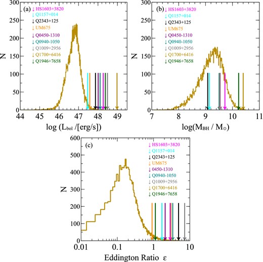
Distributions of (a) bolometric luminosity, (b) virial black hole mass, and (c) Eddington ratio for our quasars (indicated by downward arrows) and ∼17000 SDSS quasars at 2.0 ≤ z < 3.1 (Shen et al. 2011: histograms). Exact values of these parameters for our nine quasars are presented in table 1. (Color online)
The radio loudness R = fν(5 GHz)/fν(4400 Å) was also collected from the literature or calculated from FIRST radio measurements. Two quasars (Q 1157+014 and UM 675) are classifiable as radio loud (R > 10; Kellermann et al. 1989), while the other seven quasars are radio quiet.
2.5 Spectroscopic observation for HS 1603+3820
We also performed spectroscopic monitoring observations of a single mini-BAL quasar (HS 1603+3820) using the 188 cm Okayama Telescope with a Kyoto Okayama Optical Low-dispersion Spectrograph (KOOLS: Yoshida 2005). For these observations, we selected a VPH495 prism, which is sensitive to 4500–5400 Å and a 1|${^{\prime\prime}_{.}}$|8 slit (yielding R ∼1100). The CCD was binned every 2 × 2 pixels.
Observations were performed from 2012 September 19 to 2015 May 21 over typical monitoring intervals of three months. Useful data were acquired on 2012 September 19, 2015 May 30, 2015 February 23, and 2015 May 21 (hereafter, these four periods are referred to as epochs 1, 2, 3, and 4). The observing log is listed in table 3.
3 Results
This section presents the photometric variability results of each quasar determined from light curves. The quasar variability properties of the mini-BAL and NAL quasars are then compared by SFs and color variability analysis. The results are summarized in figures 2 and 3 and in table 4.
![Light curves of four mini-BAL quasars [(a) HS 1603+3820, (b) Q 1157+014, (c) Q 2343+125, and (d) UM 675], monitored in the u (open squares), g (filled squares), and i bands (open circles). The horizontal axis denotes the observing date (year-month) and the vertical axis Δm is the magnitude difference from the first observation. The Δm first observing epoch is zero by definition.](https://oup.silverchair-cdn.com/oup/backfile/Content_public/Journal/pasj/68/4/10.1093_pasj_psw044/4/m_pasj_68_4_48_f2.jpeg?Expires=1750230261&Signature=gqCMreawTUztd2bJ0m1Xe58oWhJkfamMdK0fHD0wcg3ubreREUH7NwrD~zYLlmoyY1sp6glqnEZQA4NKi-u9aiQ9v9joz05zM3jSDXlUyoDFqyQGBEXpXA38i6qJL0MQS-RDo~zcUuX8EOjOC9V32ggeBwKS4eXzmMFC6KQX9SYPSe-fZP7bYSK20Np-XSnQr8bCC2DYjyol68rdA8Bc8IQv5KoMt571UFG0rJLEpdEibbf7vD0ZyyLgVSsuymgWz9UVC04zKuhngz6tvAU5dqJzZ28kBgo50B34zUoTy0x6xkD50zu3Bg19NTVdVfTCmLFiDwa4rchxx7RuK6LRzQ__&Key-Pair-Id=APKAIE5G5CRDK6RD3PGA)
Light curves of four mini-BAL quasars [(a) HS 1603+3820, (b) Q 1157+014, (c) Q 2343+125, and (d) UM 675], monitored in the u (open squares), g (filled squares), and i bands (open circles). The horizontal axis denotes the observing date (year-month) and the vertical axis Δm is the magnitude difference from the first observation. The Δm first observing epoch is zero by definition.
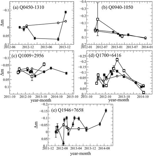
Identical to figure 2, but plotted for the five NAL quasars, (a) Q 0450−1310, (b) Q 0940−1050, (c) Q 1009+2956, (d) Q 1700+6416, and (e) Q 1956+7658.
3.1 Quasar variability
To examine the quasar variability of the nine mini-BAL/NAL quasars, we measured the standard deviation in the magnitude σm, the mean quasar variability 〈|Δm|〉, the maximum magnitude variability |Δm|max, the mean quasar variability gradient 〈|Δm/Δtrest|〉, and the maximum quasar variability gradient |Δm/Δtrest|max, following Borgeest and Schramm (1994) and G99. The mean values were calculated from all combinations of the observing epochs (e.g., from NC2 combinations, where N is the number of observing epochs). The quasar variability gradient was defined as the quasar variability per unit time (year). These parameters are summarized in table 4. The maximum quasar variability and its gradient are listed even if their significance level is below 3 σ.
The most remarkable trend is the larger quasar variabilities in bluer bands than those in redder bands. This well-known property of quasars is repeatedly discussed in the literature (e.g., Cristiani et al. 1997; VB04; Zuo et al. 2012; Guo & Gu 2014). The largest quasar variabilities were exhibited by HS 1603+3820 among the mini-BAL quasars (|Δumax| ∼ 0.23) and by Q 1700+6416 among the NAL quasars (|Δumax| ∼ 0.30), while the largest variability gradients were exhibited by Q 1157+014 among the mini-BAL quasars (|Δi/Δtrest|max ∼ 5.0) and by Q 1946+7658 among the NAL quasars (|Δg/Δtrest|max∼ 16.9).
3.2 Notes on individual quasars
3.2.1 HS 1603+3820 (mini-BAL, zem = 2.542, mV = 15.9)
This quasar exhibited a violently variable mini-BAL profile with an ejection velocity v ∼ 9500 km s−1 (Misawa et al. 2007b). Among the mini-BAL quasars in the present study, this quasar showed the largest variability in the u band (|Δu| ∼ 0.23 mag) and the second largest variability in the g band (|Δg| ∼ 0.19 mag) among our mini-BAL quasars. On the other hand, the mean and maximum quasar variability of HS 1603+3820 were surprisingly small in the i band (only ∼0.01 and ∼0.05 mag, respectively). For this quasar alone, we supplemented the photometric observations with spectroscopic observations. The C iv mini-BALs in this quasar obtained in each epoch are summarized in figure 4, and we measured the EW of the C iv mini-BAL and monitored its variability. The results are summarized in figure 5 and table 5. The EW marginally varied between epochs 1 and 3 with absorption variability amplitude ΔEW = 6.0 ± 4.2 Å (significance level ∼1.5 σ).
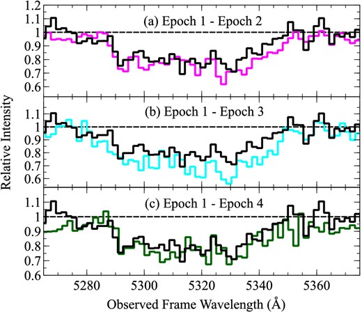
Normalized spectra of HS 1603+3820 around the C iv mini-BAL in the observed frame taken with the 188 cm Okayama Telescope. Black, magenta, cyan, and green histograms denote spectra taken on 2012 September 19 (epoch 1), 2014 May 30 (epoch 2), 2015 February 23 (epoch 3), and 2015 May 21 (epoch 4), respectively. C iv mini-BALs in (a) epoch 2, (b) epoch 3, and (c) epoch 4 are compared to the C iv mini-BAL in epoch 1. Horizontal dotted lines represent the normalized continuum levels. (Color online)

3.2.2 Q 1157+014 (mini-BAL, zem = 2.00, mV = 17.6)
This radio-loud quasar (R = 471) was the faintest among our sample quasars. At the start of our monitoring campaign, Q 1157+014 showed a rapid quasar variability in the i band with an amplitude |Δi| ∼ 0.14 mag, much larger than those of the u and g bands, between the first (2012 April) and second (2012 May) epochs. Thereafter, the magnitude variability remained high in the u band and reduced in the i band.
3.2.3 Q 2343+125 (mini-BAL, zem = 2.515, mV = 17.0)
This quasar exhibited the largest Eddington ratio ε among our mini-BAL quasars (ε ∼ 4.90) and the smallest mean quasar variability in the g band (〈|Δg|〉 ∼ 0.02). The quasar variability was only slightly larger in the i band than in the g band. Although Q 2343+125 was observed only twice in the u band, precluding an evaluation of its variability trend in that band, it appears that the quasar variability trends were consistent in all three bands.
3.2.4 UM 675 (mini-BAL, zem = 2.15, mV = 17.1)
This radio-loud quasar (R = 438) has a sub-Eddington luminosity (ε = 0.91) and exhibited the largest variability in the g and i bands among the mini-BAL quasars (|Δg| and |Δi| are ∼ 0.22 and 0.16 mag, respectively). Similar to Q 2343+125, detailed trends in the u band were precluded by the limited number of monitoring epochs.
3.2.5 Q 0450−1310 (NAL, zem = 2.30, mV = 16.5)
The magnitude of this quasar suddenly changed (|Δg| ∼ 0.16 mag) in the g band during the last three months of observations (from 2013 September to 2013 December). The Δm in the g and i bands largely differed from the third to the fifth observing epochs, possibly because there were few observing epochs in the i band.
3.2.6 Q 0940−1050 (NAL, zem = 3.080, mV = 16.6)
The g- and i-band fluxes monotonically decreased during the monitoring campaign. The quasar variability amplitudes of all the bands were almost identical. In this case, the variable trend in the u band was obscured by the large photometric error, especially in the second epoch. These errors were introduced by bad weather.
3.2.7 Q 1009+2956 (NAL, zem = 2.644, mV = 16.0)
Among our samples, this NAL quasar has the largest Eddington ratio (ε = 7.21) and the smallest variability level in all bands (|Δm| ≤ 0.06 mag).
3.2.8 Q 1700+6416 (NAL, zem = 2.722, mV = 16.13)
The bolometric luminosity and black hole mass of this quasar were the largest among our samples. Q 1700+6416 also exhibited the largest u-band variability (|Δu| ∼ 0.3 mag) among our samples.
3.2.9 Q 1946+7658 (NAL, zem = 3.051, mV = 15.85)
This quasar exhibited a cyclic quasar variability pattern with the highest half-year variability of the g-band magnitude in the quasar rest frame (|Δg| ∼ 0.24 mag). Conversely, the i-band magnitude was very stable over the same observation term.
3.3 Structure function analysis
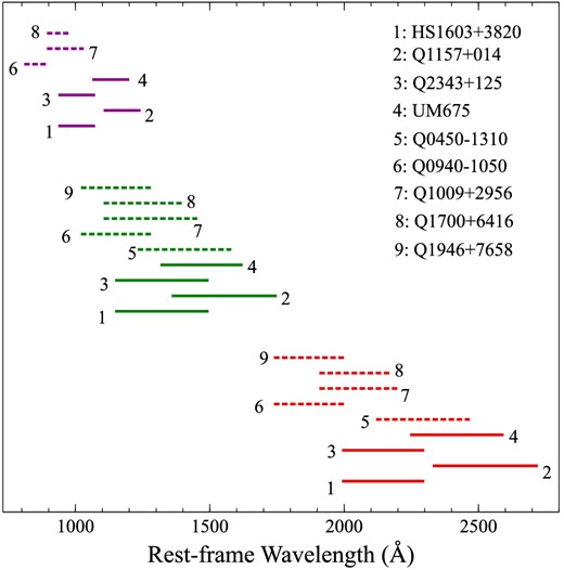
Regions of rest-frame wavelength covered by SDSS u (violet), g (green), and i (red) bands for each quasar. The solid and dotted lines represent the wavelength coverage of mini-BAL and NAL quasars, respectively. The quasars covering each wavelength range are labeled 1–9. (Color online)
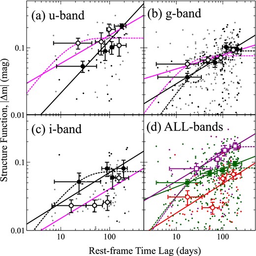
Structure functions of (a) u band, (b) g band, and (c) i band of mini-BAL (filled circles) and NAL (open circles) quasars, plotted on a log–log scale. The statistical error in the SF includes the error propagation. Horizontal error bars indicate the variances from the mean time intervals in each bin. In panels (a), (b), and (c), the quasar variabilities of mini-BAL (black dots) and NAL (gray dots) quasars are plotted for all combinations of the observing epochs. The SFs of the mini-BAL (black lines) and NAL (magenta lines) quasars are fitted by a power law (solid line) and an asymptotic function (dotted line), respectively. (d) The SFs of all subsamples including mini-BAL and NAL quasars in the u band (violet), g band (green) and i band (red) are also fitted to power-law and asymptotic functions. The quasar variabilities of all our quasars in the u band (violet dots), g band (green dots), and i band (red dots) are also plotted for all combinations of the observing epochs. Unsatisfactory fitting results are omitted. (Color online)
Power-law and asymptotic fitting parameters of structure functions.
| Quasars | Reference | S p | S a | ||
|---|---|---|---|---|---|
| γ | S(Δτ = 100 d) | Δτa (Asymptotic) | V a | ||
| (mag) | (d) | (mag) | |||
| SDSS u band | |||||
| mini-BAL quasars | this work | 0.785 ± 0.109 | 0.129 ± 0.037 | –† | –† |
| NAL quasars | this work | 0.422 ± 0.345 | –* | 12.282 ± 10.090 | 0.139 ± 0.026 |
| All of our quasars | this work | 0.410 ± 0.115 | 0.135 ± 0.076 | 49.362 ± 15.210 | 0.169 ± 0.019 |
| SDSS 7886 quasars | W08 | 0.435 | 0.173 ± 0.001 | – | – |
| SDSS g band | |||||
| mini-BAL quasars | this work | 0.426 ± 0.078 | 0.078 ± 0.036 | 37.980 ± 15.640 | 0.090 ± 0.016 |
| NAL quasars | this work | 0.210 ± 0.071 | 0.078 ± 0.067 | 13.537 ± 6.981 | 0.076 ± 0.008 |
| All of our quasars | this work | 0.264 ± 0.056 | 0.080 ± 0.043 | 20.768 ± 7.478 | 0.082 ± 0.008 |
| SDSS 25710 sample | VB04 | 0.293 ± 0.030 | – | 51.9±6.0‡ | 0.168 ± 0.005 |
| SDSS 7886 quasars | W08 | 0.479 | 0.147 ± 0.001 | – | – |
| SDSS i band | |||||
| mini-BAL quasars | this work | 0.446 ± 0.263 | –* | 18.870 ± 9.088 | 0.073 ± 0.008 |
| NAL quasars | this work | 0.432 ± 0.111 | –* | –* | –* |
| All of our quasars | this work | 0.432 ± 0.121 | –* | –† | –† |
| SDSS 25710 sample | VB04 | 0.303 ± 0.035 | – | 62.6 ± 8.3‡ | 0.139 ± 0.005 |
| SDSS 7886 quasars | W08 | 0.436 | 0.108 ± 0.001 | – | – |
*Unphysical values were obtained.
†The data cannot be properly fitted by an asymptotic function.
‡Data in VB04 not explicitly given to two decimal places.
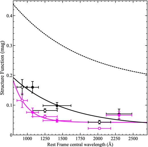
Structure function versus rest-frame wavelength. The samples were first separated into two subsamples with longer and shorter time lags. The separation criterion was Δτ = 90 d in the rest frame. Filled and open circles (magenta: Δτ < 90, black: Δτ > 90) indicate the SFs of mini-BAL and NAL quasars, respectively. For each mini-BAL/NAL quasar, the rest-frame central wavelength denotes the average central (rest-frame) wavelengths among all bands. Horizontal error bars indicate the bandwidth of each filter. Solid black (Δτ > 90) and magenta (Δτ < 90) curves are the fitting results. The black dotted curve is fitted to the ∼25000 normal quasars from VB04 data by equation (7) (A = 0.616 ± 0.056, λ0 = 988 ± 60, B = 0.164 ± 0.003). (Color online)
3.4 Color variability
Figure 9 plots the Δ(u − g), Δ(u − i), and Δ(g − i) color variabilities as functions of quasar variability. The correlation properties of the mini-BAL and NAL quasars are summarized in table 7. The color and magnitude variabilities are positively correlated in both mini-BAL and NAL quasars (namely, brighter quasars tend to be bluer; hereafter called the BWB trend). The same phenomenon has been reported in normal quasars (e.g., G99; Webb & Malkan 2000; VB04; Sakata et al. 2010, 2011; Kokubo et al. 2014). The correlation trends are consistent in the mini-BAL and NAL quasars.
![Color variability of Δ(u − g) (top), Δ(u − i ) (middle), and Δ(g − i ) (bottom) versus magnitude variability in mini-BAL [left column: (a), (b), and (c)] and NAL [right column: (d), (e), and (f)] quasars. Magnitude variabilities were determined in the bluer bands. Solid lines are the best fits to the distributions. (Color online)](https://oup.silverchair-cdn.com/oup/backfile/Content_public/Journal/pasj/68/4/10.1093_pasj_psw044/4/m_pasj_68_4_48_f9.jpeg?Expires=1750230261&Signature=yMoHqcww3E-bn1LWr1Hs4~JYtd-HFRdQNKBcgTmFaExyxVTiwpHBe9feppy0d5yIZstI5UoEqZB4o-IfM5HbJ8PRhlzEt5ZRHiz2etl~~abHcFKYkjZrca0LybrP3RVSLgHPXN6aXGBPSNphsnXWWomTPsP9MoymCqJXxnXi~srqV6zAkzSWEkYpJNQ~m6UlOTYsXOhjLi342NGQN7SycAJj5XyZQspUoQdePjlR8FuaSM~poCH-IDCvHvyxw-bUpu22RvofjZhKs4C~iyf7Se7Lb62dIGq8VgQq0Go-TAyf~DWtGNEwl~F4mW0E-XA5h64GrmOUjr5TWQhXb3a1UA__&Key-Pair-Id=APKAIE5G5CRDK6RD3PGA)
Color variability of Δ(u − g) (top), Δ(u − i ) (middle), and Δ(g − i ) (bottom) versus magnitude variability in mini-BAL [left column: (a), (b), and (c)] and NAL [right column: (d), (e), and (f)] quasars. Magnitude variabilities were determined in the bluer bands. Solid lines are the best fits to the distributions. (Color online)
The standard deviations of the quasar colors, the mean and maximum color variabilities, and the mean and maximum color variability gradients of the mini-BAL and NAL quasars are listed in table 8. Again, no significant differences exist between the mini-BAL and NAL quasars, except for 5.4 σ difference in the maximum color gradient of Δ(u − i).
4 Discussion
4.1 Quasar variability trends of mini-BAL and NAL quasars
4.1.1 Structure function
Comparing the SF fitting parameters of the mini-BAL and NAL quasars to those of normal quasars reported in VB04 and W08 (table 6), we observe the following trends:
The power-law indices γ of the mini-BAL and NAL quasars (γ ∼ 0.410 ± 0.115, 0.264 ± 0.056, and 0.436 ± 0.115) were consistent with those of normal quasars reported in W08 (γ ∼ 0.43, 0.48, and 0.44) except in the g band, although the rest-frame wavelength coverage differed among the quasar samples (being dependent on the redshift distribution of the quasar). Similar indices were obtained in a disk instability model5 (γ = 0.41 ∼ 0.49; Kawaguchi et al. 1998). No significant differences were observed between the mini-BAL and NAL quasars.
In the asymptotic model Va, the asymptotic value at Δτ = ∞ of mini-BAL/NAL quasars was approximately half that of normal quasars in the g and i bands. The same phenomenon was observed for S(Δτ = 100 d).
4.1.2 Color variability
The mini-BAL and NAL quasars exhibit similar color-magnitude variability (table 7) and color variability (table 8) with one exception: a 5.4 σ difference in the maximum color gradients [MCGs; (|ΔC/Δtrest|)max].
Distribution properties of color variability versus quasar variability.
| Distribution | N* | r † | a ‡ |
|---|---|---|---|
| mini-BAL quasar | |||
| Δ(u − g)–Δu | 21 | 0.821 | 0.527 ± 0.064 |
| Δ(u − i)–Δu | 14 | 0.781 | 1.034 ± 0.121 |
| Δ(g − i)–Δg | 26 | 0.570 | 0.674 ± 0.048 |
| NAL quasar | |||
| Δ(u − g)–Δu | 28 | 0.891 | 0.601 ± 0.041 |
| Δ(u − i)–Δu | 22 | 0.962 | 0.741 ± 0.042 |
| Δ(g − i)–Δg | 64 | 0.882 | 0.830 ± 0.038 |
*Number of data points.
†Pearson product-moment correlation coefficient.
‡Slope of regression line.
Color variability properties of mini-BAL and NAL quasars.
| Color | σΔc* | 〈ΔC〉† | |ΔCmax|‡ | Quasar§ | 〈ΔC/Δtrest〉‖ | (|ΔC/Δtrest|)max♯ | Quasar** |
|---|---|---|---|---|---|---|---|
| (mag) | (mag) | (mag) | (mag yr−1) | (mag yr−1) | |||
| mini-BAL quasar | |||||||
| Δ(u − g) | 0.057 | 0.058 ± 0.010 | 0.184 ± 0.051 | Q 1157+014 | 0.161 ± 0.040 | 0.718 ± 0.200 | UM 675 |
| Δ(u − i) | 0.069 | 0.092 ± 0.016 | 0.241 ± 0.046 | Q 1157+014 | 0.305 ± 0.048 | 0.482 ± 0.104 | HS 1603+3820 |
| Δ(g − i) | 0.038 | 0.051 ± 0.007 | 0.136 ± 0.023 | Q 1157+014 | 0.174 ± 0.028 | 3.952 ± 0.621 | Q 1157+014 |
| NAL quasar | |||||||
| Δ(u − g) | 0.047 | 0.071 ± 0.009 | 0.182 ± 0.025 | Q 1700+6416 | 0.170 ± 0.034 | 1.956 ± 0.609 | Q 1700+6416 |
| Δ(u − i) | 0.060 | 0.080 ± 0.013 | 0.218 ± 0.022 | Q 1700+6416 | 0.188 ± 0.046 | 1.374 ± 0.129 | Q 1700+6416 |
| Δ(g − i) | 0.049 | 0.048 ± 0.006 | 0.208 ± 0.022 | Q 1946+7658 | 0.107 ± 0.025 | 5.329 ± 0.584 | Q 1946+7658 |
*Standard deviation of color amplitude.
†Mean amplitude of color variability.
‡Maximum amplitude of color variability.
§Quasar with maximum color variability amplitude.
‖Mean color variability gradient (per year).
♯Maximum color variability gradient (per year).
**Quasar with maximum color variability gradient.
The 5.4 σ difference in MCGs was observed between a mini-BAL quasar (HS 1603+3820) and a NAL quasar (Q 1700+6416) with BWB trends in Δ(u − i). In both quasars, the variability was maximum in the u band and moderate in the i band. However, the u − i variability developed over a shorter time frame in Q 1700+6416 than in HS 1603+3820, which might explain the larger color variability gradient in the former than in the latter.
4.1.3 Correlation between EW and quasar variability
As shown in figure 5, the variability trends of the magnitude and EW of the C iv mini-BAL for HS 1603+3820 were marginally synchronized with the quasar variability leading the EW variability. Specifically, the EW first increased from 2012 September (epoch 1) to 2015 February (epoch 3) with a marginal significance level of ∼1.5 σ (ΔEW = 6.0 ± 4.2) and then decreased from 2015 February to 2015 May (epoch 4), while the quasar brightness in the u band first decreased from 2012 September to 2014 May and then increased from 2014 May to 2015 May. The time lag of the marginal synchronizing trend in quasar and absorption line variabilities is about nine months (∼2.6 mon in the quasar rest frame). If we assume the time delay corresponds to the recombination time from C v to C iv, we can place a lower limit on the absorber's gas density of ne ≥ 2.8 × 104 cm−3 by the same prescription as used in Narayanan et al. (2004).
Trévese et al. (2013) reported a similar synchronizing trend in a BAL quasar APM 08279+5255, although one of two NALs detected aside the BAL did not show such a synchronization. They suggested this was due to a larger recombination time for the NAL absorber with smaller electron density compared to the other absorbers. Both of these results are not inconsistent with the VIS scenario.
4.2 The VIS scenario
Here, we assume the absorption line variability of (mini-)BALs is attributed to recombination to (or ionization from) C2 + (case A, hereafter) and adopt the optimal ionization parameters for C2 + and C3 + (log U ∼ − 2.8 and − 2.0, respectively; Hamann 1997). Because at least one of our mini-BAL quasars (HS 1603+3820) is unlikely to vary by the gas motion scenario (Misawa et al. 2005, 2007b), we assume constant gas density ne. Therefore, the ionizing photon density nγ should increase/decrease by a factor of ∼6.3 to change log U from/to −2.8 to/from −2.0, corresponding to Δm ∼ 2. For reference, a typical quasar varies by only Δm ∼ 0.1 over several months and maximally varies by Δm ∼ 0.5 over several years (Webb & Malkan 2000). These variabilities are much smaller than the above-required value.6
However, C iv absorbers do not necessarily have an optimal ionization parameter for C3 + (i.e., log U ∼ −2.0). As the other extreme case, if mini-BAL absorbers have log U ∼ −3.0, their ionization fraction f (i.e., the fraction of carbon in ion state C3+) is very sensitive to the ionization parameter (Δlog f/Δlog U ∼ 1.8; case B, hereafter), although it weakly depends on the shape of incident ionizing flux. Indeed, the value of Δlog f/Δlog U for HS 1603+3820, which is the only quasar among our sample for which the magnitude and EW of the C iv mini-BAL were simultaneously monitored over three years, is ∼1.1 between epochs 1 and 2 (Δlog EW ∼Δlog f ∼ 0.1)7 and ∼2.0 between epochs 1 and 3 (Δlog EW ∼ 0.18), assuming Δm ∼ 0.23 (the maximum quasar variability during our monitoring observations). These values are expected for absorbers with ionization parameters of log U ∼ −3–2 (see figure 2 of Hamann 1997). If this is the case, an averaged amplitude of absorption variability in four C iv mini-BALs in our sample (〈Δlog EW〉 ∼ 〈Δlog f〉∼ 0.1) can be caused by only a small change of the ionizing flux, log U ∼ 0.06. This value corresponds to Δm ∼ 0.14, comparable to a typical variability of our sample quasars as well as quasars in the literature (Webb & Malkan 2000). The variability amplitude of C iv ionizing photons in shorter wavelength (λrest ∼ 200 Å) may be even larger because of the anti-correlation between quasar variability and wavelength (see subsection 3.3).
Thus, case B is favorable for explaining the variability trend in HS 1603+3820 with the VIS scenario. However, it has one shortcoming; four mini-BAL systems in our sample have either strong N v absorption lines or no remarkable Si iv absorption lines, which suggests their ionization condition is not as low as log U ∼ −3 (see figure 2 of Hamann 1997). Therefore, it is less likely that case B alone causes the absorption variability of mini-BALs in our sample quasars.
4.3 Additional mechanism to support the VIS scenario
The outflow wind variability may be caused by more than one mechanism. We speculate that the VIS scenario is accompanied by an additional mechanism, such as variable optical depth between the flux source and the absorber. One promising candidates is a warm absorber, which has frequently been detected in X-ray spectroscopy (e.g., Gallagher et al. 2002, 2006; Krongold et al. 2007; Mehdipour et al. 2012). Warm absorbers were originally proposed to avoid over-ionization of the outflow winds (Murray et al. 1995). Because warm absorbers are significantly variable in X-ray monitoring observations (e.g., Chartas et al. 2007; Giustini et al. 2010a, 2010b), the ionization condition of the UV absorber in the downstream might also vary. Indeed, in a photoionization model, Różańska et al. (2014) estimated that the C iv mini-BAL absorber lies within r = 0.1 pc of the quasar center. Similarly, the X-ray warm absorber is estimated to be within 0.1 pc of HS 1603+3820. Ganguly et al. (2001) argued that NAL and BAL absorbers locate at high and low latitudes above the accretion disk equator, respectively. A radiation–MHD simulation by Takeuchi, Ohsuga, and Mineshige (2013) also predicts no warm absorbers at very high latitudes. If this picture is correct, X-ray shielding is ineffective in the NAL outflow directions. Supporting this idea, X-rays are not strongly absorbed in NAL quasars (Misawa et al. 2008). The model of Kurosawa and Proga (2009) supports that NAL absorbers are the interstellar media of host galaxies, which are swept up by the outflow wind. In this case, the absorbers should exhibit little variability because their volume density is very small (corresponding to a very long recombination time). Moreover, they are very distant (of the order of kpcs) from the continuum source, and therefore they should be weakly influenced by the variable flux source. However, Hamann et al. (2013) find no evidence of strong X-ray absorption toward the outflows of either NAL or mini-BAL quasars. Instead of an X-ray warm absorber, they argue that small dense clumpy absorbers avoid over-ionization by self-shielding. In this case, we should expect no correlations between the absorption strengths of the UV and X-ray fluxes.
5 Summary
We performed (i) photometric monitoring observations of four mini-BAL and five NAL quasars over more than three years, and (ii) spectroscopic observation for a single mini-BAL quasar (HS 1603+3820) to investigate whether the VIS scenario can explain the absorption line variability in BALs and mini-BALs. Our main results are summarized below:
Quasar variability increases with monitoring time lag but decreases with observed wavelength, as previously reported in normal quasars.
Mini-BAL and NAL quasars become bluer as they brighten (the BWB trend), as often observed in normal quasars.
The quasar variability properties did not significantly differ between mini-BAL and NAL quasars, indicating that flux and color variabilities alone cannot account for the absorption line variabilities.
Quasar magnitude was marginally synchronized with absorption strengths in one mini-BAL quasar HS 1603+3820, with the former temporally leading the latter.
The VIS scenario cannot cause the absorption variability of mini-BALs in our sample quasars unless the ionization condition of outflow gas is as low as log U ∼ −3.
The VIS scenario may require an additional mechanism that regulates incident flux to the outflow gas. The most promising candidate is X-ray warm absorbers with variable optical depth.
Before conclusively validating the VIS scenario, we need to simultaneously monitor the outflow and shielding material by UV and X-ray spectroscopy. The presented monitoring observations should also be performed on quasars with a wide range of luminosities and Eddington ratios to mask the anti-correlation effect between the luminosity/Eddington ratio and quasar variability.
We thank Ken'ichi Tarusawa, Takao Soyano, and Tsutomu Aoki for supporting our observations at Kiso Observatory for over three years. Ikuru Iwata and Hironori Tsutsui supported our observations with the 188 cm Okayama Telescope with KOOLS. We also thank Noboru Ebizuka, Masami Kawabata, and Takashi Teranishi for producing VPH grisms used in KOOLS and kindly providing them to us, and Rina Okamoto for supporting our observations at Kiso Observatory and Okayama Astrophysical Observatory. The research was supported by JGC-S Scholarship Foundation and the Japan Society for the Promotion of Science through Grant-in-Aid for Scientific Research 15K05020.
On the other hand, changes in the absorption strength/feature are referred to as “absorption line variability.”
We emphasize that the rest-frame wavelength regions studied in the current work may differ from those in the literature.
The average time lag of all combinations of observing epochs in all bands (used as the criterion).
Transient flares or blob formations caused by any instability should alter the luminosity.
Even if we attribute the absorption line variability to recombination to (or ionization from) C v (whose optimal ionization parameter is log U ∼ −1.2), the required magnitude variability would be almost the same.
If absorbing clouds are optically thin (i.e., absorption lines are at a linear part of the
curve of growth), Δlog EW is close to Δlog f, which is applicable for all mini-BALs in our sample except for one in Q 1157+014.
References
