


Abstract
We perform image stacking analysis of Sloan Digital Sky Survey (SDSS) photometric galaxies over the AKARI Far-Infrared Surveyor maps at 65 μm, 90 μm, and 140 μm. The resulting image profiles are decomposed into the central galaxy component (single term) and the nearby galaxy component (clustering term), as a function of the r-band magnitude, mr, of the central galaxy. We find that the mean far-infrared (FIR) flux of a galaxy with magnitude mr is well fitted with |$f^s_{90\mu {\rm m}}=13\times 10^{0.306(18-m_{\,r})}$| [mJy]. The FIR amplitude of the clustering term is consistent with that expected from the angular-correlation function of the SDSS galaxies, but galaxy morphology dependence needs to be taken into account for a more quantitative conclusion. We also fit the spectral energy distribution of stacked galaxies at 65 μm, 90 μm, and 140 μm, and derive a mean dust temperature of ∼30 K. This is consistent with the typical dust temperature of galaxies that are FIR luminous and individually detected.
1 Introduction
Dust plays an important role in the formation and chemical evolution of galaxies. Dust absorbs and scatters the ultraviolet (UV) light associated with star formation activities, and approximately re-emits half of the star light in infrared (IR; e.g., Lutz 2014). The infrared dust emission from individual galaxies, however, is very difficult to detect in IR generally, except for bright sources. This is why image stacking analysis is very useful in measuring and characterizing the IR emission from typical galaxies in a statistical fashion.
Recently, for instance, Kashiwagi, Yahata, and Suto (2013, hereafter KYS13) performed stacking analysis of SDSS (York et al. 2000) photometric galaxies over the Galactic extinction map by Schlegel, Finkbeiner, and Davis (1998, hereafter SFD). The SFD extinction map is basically constructed from the InfraRed Astronomical Satellite (IRAS)/IRAS Sky Survey Atlas (ISSA) far-infrared (FIR) emission map at 100 μm with dust temperature correction using the Cosmic Background Explorer (COBE) data.
KYS13 were originally motivated to explain the anomaly of the SFD extinction map (Yahata et al. 2007; Kashiwagi et al. 2015) in terms of FIR emission contamination from galaxies. Indeed, they were successful in detecting the additional extinction statistically over the SFD map that should be ascribed to SDSS galaxies. Any further quantitative interpretation of the result, however, is limited by the poor angular resolution (FWHM ∼6′) of the IRAS 100 μm map.
In this paper, we perform similar stacking analysis using the Far-Infrared Surveyor (FIS: Doi et al. 2015; Takita et al. 2015) on board the Japanese infrared satellite AKARI (Murakami et al. 2007). FIS covers almost 98% of the whole sky with a spatial resolution of ∼ 1|${^{\prime}_{.}}$|5, approximately four times better than that of IRAS. Also, FIS maps at 65, 90, 140, and 160 μm are useful in estimating the corresponding dust temperature in a statistical fashion. Indeed, the longer wavelength bands correspond to the peak of dust far-infrared emission from SDSS photometric galaxies, as described below.
The present paper is organized as follows. Section 2 briefly summarizes the AKARI FIS all-sky map and SDSS DR7 photometric galaxy catalog that we use throughout the current analysis. Section 3 describes the point spread functions (PSFs) of FIS, and also presents the stacking method. of the stacking. The stacked images at 90 μm are fitted to the model profiles in section 4, and compared with prediction on the basis of the angular-correlation function of SDSS galaxies in section 5. We repeat a similar stacking analysis at 65 and 140 μm, and derive the dust temperature of SDSS galaxies in section 6. Finally, section 7 is devoted to a summary and the conclusion of the paper.
2 Data: SDSS and AKARI FIS
Our stacking analysis utilizes the two datasets AKARI FIS (Kawada et al. 2007) and SDSS DR7 data (Abazajian et al. 2009), which we describe briefly below.
2.1 AKARI FIS all-sky maps
FIS is an instrument on board the AKARI satellite (Kawada et al. 2007). It has four photometric bands at 65 μm, 90 μm, 140 μm, and 160 μm, and covers almost all the sky. Figure 1 shows the 90 μm image of the FIS map in ecliptic coordinates. The absolute calibration of the FIS map is based on comparison with the COBE/DIRBE (Diffuse Infrared Background Experiment) data (Takita et al. 2015). While other components and point sources are not removed, smooth cloud components of the zodiacal emission are subtracted from the map following Gorjian, Wright, and Chary (2000). Indeed, a faint signature of the residual zodiacal light is visible around the equator in figure 1.
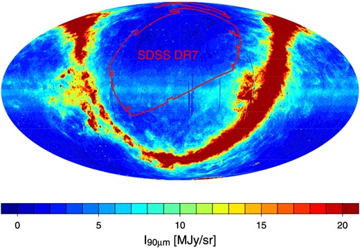
All-sky map of 90 μm observed by AKARI in ecliptic coordinates. The color scale indicates the intensity of FIR emission at 90 μm. The region surrounded by the red solid line indicates the SDSS DR7 survey region used in the north Galactic map for the present analysis. (Color online)
The point-source detection levels of the survey mode at a signal-to-noise ratio of 5 σ are 2.4 Jy, 0.55 Jy, and 1.4 Jy at 65 μm, 90 μm, and 140 μm, respectively (Kawada et al. 2007). Arimatsu et al. (2014) directly measure the PSFs of FIS by stacking infrared standard stars of Cohen et al. (1999). Their catalogue includes 422 giant stars with spectral types of K0 to M0, and Arimatsu et al. (2014) stack 80% of those stars. Table 1 summarizes the values of the PSFs of FIS and the 5 σ detection limits in each wavelength. The PSFs of FIS are elongated along the direction of scanning because of the slow response of the FIS detector. This is why we show three different values for the full width at half maximum (FWHM) in table 1: along the scan direction (In-scan), perpendicular to the scan direction (Cross-scan), and their circular average. Since the 160 μm data are too noisy, we do not use them (cf. Arimatsu et al. 2014).
FWHMs of the PSFs of AKARI FIS* and the 5 σ detection limits at each wavelength.
| 65 μm | 90 μm | 140 μm | |
|---|---|---|---|
| In-scan FWHM | 82″ | 98″ | 101″ |
| Cross-scan FWHM | 33″ | 55″ | 70″ |
| Circular average FWHM | 53″ | 73″ | 86″ |
| 5 σ detection limit | 2.4 Jy | 0.55 Jy | 1.4 Jy |
| 65 μm | 90 μm | 140 μm | |
|---|---|---|---|
| In-scan FWHM | 82″ | 98″ | 101″ |
| Cross-scan FWHM | 33″ | 55″ | 70″ |
| Circular average FWHM | 53″ | 73″ | 86″ |
| 5 σ detection limit | 2.4 Jy | 0.55 Jy | 1.4 Jy |
* Obtained from table 2 of Arimatsu et al. (2014).
2.2 SDSS DR7 photometric galaxies
Our stacking analysis is based on the SDSS DR7 (Abazajian et al. 2009) photometric galaxy catalog, which covers 11663 deg2 of the sky, with photometry in five passbands: u, g, r, i, and z. (See Fukugita et al. 1996; Gunn et al. 1998, 2006; Hogg et al. 2001; Stoughton et al. 2002; Smith et al. 2002; Pier et al. 2003; Ivezić et al. 2004; Tucker et al. 2006; Padmanabhan et al. 2008 for more details of the photometric data.) We use the contiguous regions of 7270 deg2 in the north galactic hemisphere (shown in figure 1). We exclude the masked regions so as to avoid those objects with unreliable photometry.
Since the spatial distribution of the Galactic stars is likely to be correlated with that of the Galactic dust, the contamination of stars in our galaxy sample would affect the interpretation of the stacking analysis presented below. Therefore, to ensure reliable star–galaxy separation, we conservatively remove bad photometry data and fast-moving objects from the “GALAXY” sample on the basis of the SDSS photometry flag; see Yahata et al. 2007 for more details of our galaxy sample selection.
Finally, we restrict the magnitude range of our galaxy sample to 15.5 < mr < 20.5. This is because the star–galaxy separation by the SDSS photometry pipeline works well for those objects with mr < 21 (Yasuda et al. 2001). Our sample selection mentioned above removes 24%–39% of the photometric galaxy candidates in each magnitude bin (table 2).
Number of SDSS galaxies used for the stacking analysis, and removed by masking the panels with I90μm > 200 [MJy sr−1] for different r-band magnitudes.
| m r | GALAXY | Selected | Stacked | Removed |
|---|---|---|---|---|
| 15.5–16.0 | 56183 | 34322 | 34315 | 7 |
| 16.0–16.5 | 100414 | 61392 | 61383 | 9 |
| 16.5–17.0 | 171767 | 108553 | 108514 | 39 |
| 17.0–17.5 | 291599 | 194546 | 194490 | 56 |
| 17.5–18.0 | 499741 | 345168 | 345078 | 90 |
| 18.0–18.5 | 861461 | 617291 | 617126 | 165 |
| 18.5–19.0 | 1476678 | 1099475 | 1099154 | 321 |
| 19.0–19.5 | 2511481 | 1909836 | 1909289 | 547 |
| 19.5–20.0 | 4208480 | 3179658 | 3178776 | 882 |
| 20.0–20.5 | 6945931 | 5042565 | 5041111 | 1454 |
3 Method of stacking analysis
3.1 Point spread function
Since the PSFs of AKARI FIS are much larger than the typical size of SDSS galaxies, each single galaxy on the stacked image is approximated by the PSFs. Therefore, it is crucially important to model the PSFs accurately. In reality, while the PSFs of AKARI FIS are elongated along the scan directions which align with ecliptic longitudes, we use their circular averages in the following analysis just for simplicity. Since Arimatsu et al. (2014) do not find any systematic dependence of the PSFs on the fluxes of the sources, we ignore the dependence on the source flux and adopt the same PSF independently of mr of galaxies.
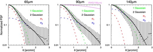
Circular-averaged PSFs at 65 μm (left), 90 μm (center), and 140 μm (right). The symbols indicate the PSFs measured by Arimatsu et al. (2014). The quoted error bars represent rms in each circular bin. The green dashed line and black solid line indicate best fits of a single Gaussian and a double Gaussian, respectively. The red and blue dashed line correspond to two components of a double Gaussian. The violet solid line in the middle panel represents the PSF of IRAS (100 μm). (Color online)
Best-fit parameters of the PSF at each passband of FIS.
| 65 μm | 90 μm | 140 μm | |
| A | 0.78 | 0.77 | 0.38 |
| σ1 | 25|${^{\prime\prime}_{.}}$|0 | 27|${^{\prime\prime}_{.}}$|7 | 22|${^{\prime\prime}_{.}}$|7 |
| σ2 | 65|${^{\prime\prime}_{.}}$|8 | 73|${^{\prime\prime}_{.}}$|8 | 54|${^{\prime\prime}_{.}}$|5 |
| 65 μm | 90 μm | 140 μm | |
| A | 0.78 | 0.77 | 0.38 |
| σ1 | 25|${^{\prime\prime}_{.}}$|0 | 27|${^{\prime\prime}_{.}}$|7 | 22|${^{\prime\prime}_{.}}$|7 |
| σ2 | 65|${^{\prime\prime}_{.}}$|8 | 73|${^{\prime\prime}_{.}}$|8 | 54|${^{\prime\prime}_{.}}$|5 |
3.2 Stacking method
Since the detection limits of SDSS are much deeper than those of FIS, the majority of the SDSS galaxies cannot be individually resolved in the FIS maps. The stacking analysis on the FIS maps, however, enables us to statistically measure the average FIR emission of the SDSS galaxies. Our method for the stacking analysis is basically the same as that adopted by KYS13, except that we mask several bright objects and subtract the zodiacal and Galactic foreground, as described below.
Consider first the 90 μm data. We divide the entire sample of SDSS galaxies according to their r-band magnitude and stack 20′ × 20′ images of the FIS map centered at the positions of SDSS galaxies in each magnitude bin. In this procedure, we evaluate the value of I90μm on 6″ × 6″ pixels over the 20′ × 20′ images, adopting a cloud-in-cell linear interpolation of the four nearest neighbors in the 15″ × 15″ pixels of the original FIS data. We first stack those images fixing the y-direction to the ecliptic longitudes so as to retain the anisotropic PSF of the FIS. Since the FIS map does not remove point sources, unlike the SFD data, we exclude those images that contain pixels with I90μm > 200 MJy sr−1 to avoid contamination due to bright point sources. We confirmed that our main result does not change even when we adopt I90μm > 100 MJy sr−1 or I90μm > 1000 MJy sr−1. Our criterion excludes several large nearby galaxies, and effectively masks about 2 deg2 in total. Table 2 lists the number of SDSS galaxies labelled as “GALAXY,” selected as our sample, and stacked after removing the regions with bright sources.
Figure 3 illustrates our stacking procedure in three different magnitude bins as an example. The left panels indicate the raw stacked results before circular averaging. In addition to the elongated source images, there is a systematic large-scale gradient along the y-axis, which originates from Galactic dust and residual zodiacal light.
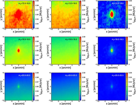
Left, middle, and right panels correspond to the raw stacked images, foreground templates, and the stacked images subtracting the foreground templates, respectively. The upper, center, and lower panels represent the results for mr = 15.5–16.0, 18.0–18.5, and 20.0–20.5, respectively. (Color online)
In order to remove the gradient component, we shift the centers of the images by +20″ and −20″ along the x-axis, i.e., constant ecliptic latitude, from the source galaxy position, and repeat the same stacking. The average of those off-source images (central panels) is used as templates of the Galactic and zodiacal foreground, and is subtracted from the corresponding raw stacked images (left panels).
The right panels of figure 3 show the stacked images after the subtraction. Clearly the large-scale gradient is successfully removed, and the signal of SDSS galaxies becomes more pronounced; note the different range of I90μm shown in the right color scales. All the analysis below is based on the stacked images corresponding to the right panels of figure 3.
4 Decomposing stacked images
Figure 4 displays the stacked images of the SDSS galaxies according to the method described in subsection 3.2 for ten different r-band magnitudes (table 2). For reference, we show the stacked image of bright stars (bottom middle panel) that should correspond to the PSF of FIS, and the stacked image on IRAS (bottom right panel) as well for comparison. The resulting stacked images exhibit prominent signatures of emission associated with the SDSS galaxies located at the origin, and indicate clearly that the angular resolution of FIS is much better than that of IRAS.
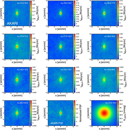
Stacked images of the AKARI FIS map for 20′ × 20′ centered at SDSS galaxies of different r-band magnitudes (mr = 15.5–20.5) in 0.5 magnitude bins. The bottom center panel corresponds to the PSF of FIS at 90 μm by Arimatsu et al. (2014). For comparison, the bottom right panel shows the stacked images of the SFD extinction map by KYS13. (Color online)
When a typical galaxy of a radius 10 kpc is located at the median redshift of the SDSS sample (〈z〉 = 0.36, Dodelson et al. 2002), the angular size is about 2″, much smaller than the size of PSFs of FIS. Thus we neglect the intrinsic size of galaxies, which is justified even visually from the comparison between the stacked galaxy and star images (figure 4).
To quantitatively characterize the FIR emission of SDSS galaxies, we compute the circular-averaged radial profiles of the stacked images, |$\Sigma _{\rm g}^{\rm tot}({\boldsymbol{\theta }};m_r)$|, in figure 5; 15.5 < mr < 16.0 (left panel) and 20.0 < mr < 20.5 (right panel).

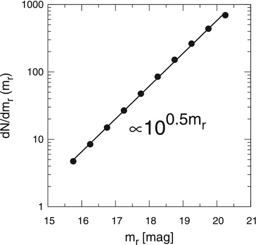
Differential number count of the SDSS galaxies as a function of r-band magnitudes. The symbols and solid line show the SDSS data and their best fit, respectively.
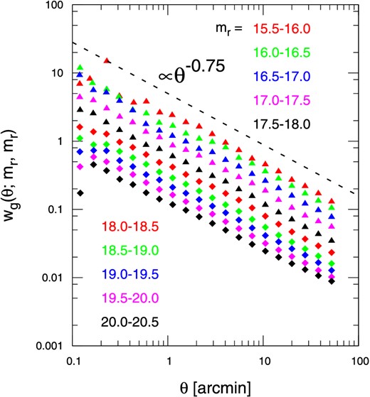
Angular correlation function of SDSS galaxies for each magnitude bin. The black dashed line indicates γ = 0.75. (Color online)
In this section, we do not use equation (7), and fit equations (2), (3), (6), and (8) to the observed circular-averaged radial profiles of the stacked images separately for each magnitude by varying the three parameters |$\Sigma _{\rm g}^{\rm s0}(m_r)$|, |$\Sigma _{\rm g}^{\rm s0}(m_r)$|, and ΔC(mr). The comparison of the resulting |$\Sigma _{\rm g}^{\rm c0}(m_r)$| with equation (7) will be considered in the next section.
The resulting best fits are plotted in green solid, red dashed, and blue dashed curves, respectively, in figure 5. Figure 8 shows the best fits of |$\Sigma _{\rm g}^{\rm s0}(m_r)$| and |$\Sigma _{\rm g}^{\rm c0}(m_r)$| against mr, where the quoted error bars are computed from 1000 subsamples of the jackknife resampling method. The results indicate that the single term dominates the clustering term around the center of the stacked images. This is in marked contrast to the result of KYS13 for IRAS at 100 μm; their figures 8, 9, and 10 indicate that |$\Sigma _{\rm g}^{\rm c0}(m_r)$| is significantly larger than |$\Sigma _{\rm g}^{\rm s0}(m_r)$|. Thanks to the better angular resolution of AKARI, we are able to separate the prominent emission from the central galaxy from the surrounding diffuse component due to the nearby galaxies. This also implies that the AKARI data enable us to measure the contribution of the single term more robustly, in a less model-dependent fashion. The difference between AKARI and IRAS will be discussed in detail later in this section.
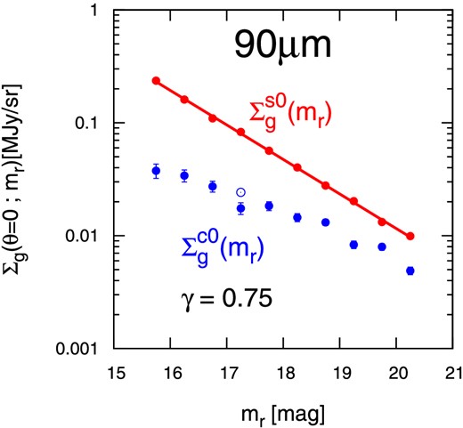
Best-fit parameters characterizing the FIR emission of galaxies against their r-band magnitude. The quoted error bars are computed from 1000 subsamples of jackknife resampling. Red and blue solid symbols indicate the best-fit values of |$\Sigma _{\rm g}^{\rm s0}(m_{\,r})$| and |$\Sigma _{\rm g}^{\rm c0}(m_{\,r})$|, respectively, assuming γ = 0.75. The red solid line indicates the best-fit line of the best-fit value of |$\Sigma _{\rm g}^{\rm s0}(m_{\,r})$| corresponding to equation (17). (Color online)
Figure 9 also indicates that ΔC in the 17.0 < mr < 17.5 bin significantly departs from the systematic trend of the other samples. A similar gap is also seen for |$\Sigma _{\rm g}^{\rm c0}(m_r)$| in figure 8. Indeed, if we use the value of ΔC in the 17.0 < mr < 17.5 bin from the interpolation of the adjacent bins (black open circle in figure 9), the resulting best fit of |$\Sigma _{\rm g}^{\rm c0}(m_r)$| also matches the other trend (blue open circle in figure 8). While we are not yet able to identify the reason for this behavior, we do not correct for this in the analysis below.
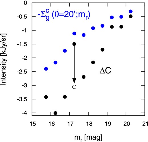
Best-fit parameters of residual constant term against their r-band magnitude (black solid symbols) and negative value of clustering term at θ = 20′, |$-\Sigma _{\rm g}^{\rm c}(\theta ={20^{\prime }};m_{\,r})$| (blue solid symbols). (Color online)
Figure 9 shows that the best-fit values of ΔC systematically increase against mr. Such mr-dependence of ΔC seems unphysical, and is likely to result from our foreground (Galactic component) subtraction procedure. Our foreground templates are computed from the stacked images at ±20′ away from the center, and thus the radial profiles of the foreground-subtracted data should vanish at θ = 20′ even though the clustering term would still extend beyond the scale. As a consequence of the over-correction, we thought that the residual of the foreground ΔC would be equal to |$-\Sigma _{\rm g}^{\rm c}(\theta =20^{\prime };m_r)$|. As shown in figure 9, however, this does not hold exactly even though the qualitative trend is consistent; the blue and black filled circles differ by a factor of two. We suspect that this difference should come from the difficulty of decomposing the weak radial dependence of the clustering term from the constant offset due to the Galactic dust in our model fit. In any case, we made sure that this dependence does not affect our main conclusion, and we do not consider it in what follows.
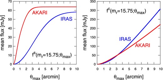
Flux of galaxies integrated within θmax for AKARI (red) and IRAS (blue). The left and right panels correspond to the flux of the single term and clustering term, respectively. (Color online)
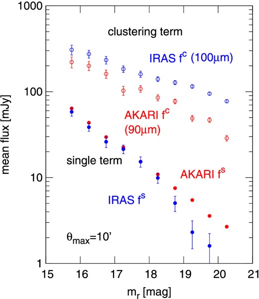
Flux of galaxies integrated up to θmax = 10′ against their r-band magnitude for AKARI (red) and IRAS (blue). The solid and open symbols indicate the flux corresponding to the single and clustering terms, respectively. (Color online)
On the other hand, the IRAS analysis for the clustering term systematically over-predicts that expected from AKARI. This should be ascribed to the difficulty of the decomposition from the lower angular resolution data of IRAS. Although the amplitudes of the clustering fluxes depend on θmax, the ratio of fluxes measured by AKARI and IRAS is independent of θmax.
Incidentally, the presence of the clustering term tends to overestimate the flux of a galaxy if not properly decomposed. Figure 12 shows the overestimate factor, [1 + f c(mr; θmax)/f s(mr; θmax)], against mr for both the IRAS and AKARI results. Here, we adopt the FWHM of PSF, 1|${^{\prime}_{.}}$|0 for AKARI and 6|${^{\prime}_{.}}$|0 for IRAS, as θmax for computing the fluxes according to equations (10) and (11). Therefore, this ratio basically indicates to what extent the flux of a single galaxy is overestimated, due to the confusion of the fluxes from neighboring galaxies within the angular resolution scales of the PSFs. Thanks to the higher angular resolution, the overestimation is significantly reduced for AKARI, but still a 50% systematic overestimate exists for mr > 18, and thus we note that the fluxes of such faint galaxies are potentially overestimated by this level.
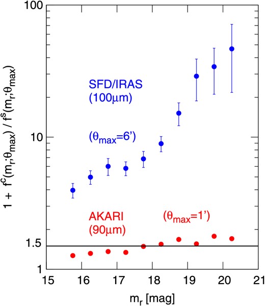
Ratio of the total flux (= f s + f c) to the single flux, f s, for both IRAS (blue) and AKARI (red). The ranges of the integral adopted are θmax = 1|${^{\prime}_{.}}$|0, 6|${^{\prime}_{.}}$|0 for AKARI and IRAS, respectively. (Color online)
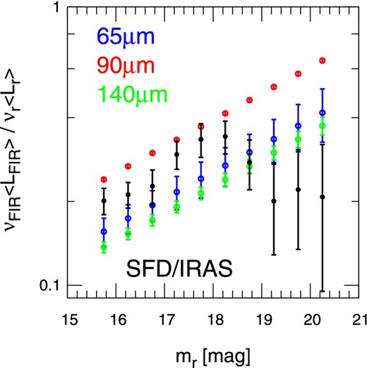
Relation between far-infrared luminosities of the central galaxy and their r-band luminosities as a function of mr. (Color online)
5 Comparison of the clustering term in FIR and the prediction from the angular correlation function of SDSS galaxies
In the last section, we estimate |$\Sigma _{\rm g, obs}^{\rm c0}(m_r)$| from the best fit to the observed profiles of the stacking images. It is interesting to compare the resulting value to the prediction from equation (7), |$\Sigma _{\rm g, model}^{\rm c0}(m_r)$|. Indeed, KYS13 carried out the comparison and suggested that the FIR fluxes for the clustering term obtained from the IRAS stacking analysis exceed those predicted from the angular correlation of the SDSS galaxies by a factor of a few. KYS13 speculate that this deficit may point to the existence of unknown FIR objects other than SDSS galaxies.
Since this has very important implications, we repeat the same analysis but with the values estimated from AKARI. As indicated in figure 11, the amplitudes of the clustering term derived from the current AKARI analysis are systematically smaller than those from IRAS. Thus the deficit discovered by KYS13 needs to be examined carefully again.
In figure 14, we plot the above result for γ = 0.75 as a black solid line, which should be compared with |$\Sigma _{\rm g,obs}^{\rm c0}(m_r)$| (filled circles with error bars). Although an overall factor of a few discrepancy in KYS13's analysis (see their figure 10) is significantly reduced, |$\Sigma _{\rm g,model}^{\rm c0}(m_r)$| is smaller than |$\Sigma _{\rm g,obs}^{\rm c0}(m_r)$| for mr < 18. In this sense, our result is still consistent with that of KYS13.
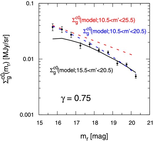
Values of the clustering terms against their r-band magnitude. The symbols, blue dashed, and red solid lines indicate the best-fit parameters from fitting and the models from SDSS data m r, min = 15.5, m r, min = 10.5, respectively. (Color online)
Nevertheless, the deficit may simply come from the upper and lower limits of the integral in equation (15). In order to evaluate equation (14), we extrapolate the functions ng(mr), |$\Sigma _{\rm g}^{\rm s0}(m_r)$|, and K(mr, m′) beyond the magnitude range of the SDSS sample.

Amplitudes of the angular correlation function of SDSS galaxies, K(m′, mr), against mr. The solid lines indicate the best-fit models of equation (18). (Color online)
We evaluate equation (14) assuming that the above extrapolation is valid. Red and blue dashed lines in figure 14 show |$\Sigma _{\rm g,model}^{\rm c0}(m_r;m_{r,\rm min}<m^{\prime }<m_{r, \rm max})$| with mr, min = 10.5 and mr, max = 20.5 and 25.5, respectively. The result suggests that |$\Sigma _{\rm g,model}^{\rm c0}(m_r)$| depends sensitively on the contribution from galaxies outside the observed magnitude range; |$\Sigma _{\rm g,model}^{\rm c0}(m_r=15.5)$| and |$\Sigma _{\rm g,model}^{\rm c0}(m_r=20.5)$| are significantly affected by galaxies with m′ < 15.5 and with m′ > 20.5, respectively. We confirmed that |$\Sigma _{\rm g,model}^{\rm c0}(m_r)$| for 15.5 < mr < 20.5 converges if we set mr, min = 10.5 and mr, max = 25.5.
Therefore, the conclusion of KYS13 that the SDSS galaxies explain less than half of the observed FIR amplitude for the clustering term is most likely due to the magnitude limit of the SDSS galaxies themselves. Indeed, if our extrapolation model is correct, the conclusion would be completely the opposite: the observed FIR fluxes are smaller than those predicted from the SDSS galaxies.
We do not take this possible discrepancy seriously, partly because it is crucially dependent on the extrapolation of the observed angular correlation function, and also partly because the galaxy morphology and redshift evolution are totally neglected here. Since dust emission from spirals is stronger than that from ellipticals, stacking analysis incorporating the morphological dependence is needed to address the above problem properly. We attempt to qualitatively consider the effect of the morphology dependence of |$\Sigma _{\rm g,model}^{\rm c0}(m_r)$| below.
For instance, if we adopt fΣ = 0.1 (Smith et al. 2012), fn = 0.6 (Rowlands et al. 2012), and fb = 2 (Skibba et al. 2009), we obtain r = 0.77. Thus our current result that |$\Sigma _{\rm g,obs}^{\rm c0}(m_r)$| is smaller than |$\Sigma _{\rm g,model}^{\rm c0}(m_r)$| may be, at least partly, accounted for by the morphological dependence of galaxies.
For reference, we repeat the above analysis by simply splitting the sample in two according to their u − r color. Following Strateva et al. 2001, we adopt u − r = 2.22 to separate the galaxy types. The number fraction of these two galaxies types is fn = 2, and the stacking analysis indicates fΣ = 0.2. While the angular correlation functions of the two types are not necessarily described by the linear bias, we take the ratio at θ = 10′ and find fb = 1.6. These yield a value of integral ratio of r = 0.84. The morphology dependence does not seem to fully explain the possible discrepancy plotted in figure 14. This indicates that the discrepancy in figure 14 may be largely due to the extrapolation of the magnitude dependence of angular correlations to fainter magnitudes. In any case, a reliable conclusion can be reached only after careful analysis in the many color bins.
6 Mean dust temperature of SDSS galaxies
Another important advantage of AKARI FIS is its multi-band coverage. From the spectrum of the stacked FIR emission in different wavelengths, we can infer the mean dust temperature of SDSS galaxies. Kashiwagi and Suto (2015) proposed a method to constrain the dust extent through the measurement of dust temperature. They obtained constraints on the dust temperature by combining the far-infrared emission computed from the stacked images of the IRAS map with the quasar reddening measurement by Menard et al. (2010). The mean spectrum energy distribution of stacked SDSS galaxies is a more direct probe of the dust temperature and independent of the method proposed by Kashiwagi and Suto (2015).
We repeat the same stacking analysis over AKARI FIS maps at 65 and 140 μm in addition to at 90 μm as described in the previous sections. In particular, 140 μm band is suited to the determination of the dust temperature because it is closer to the expected peak of the dust emission.
Figure 16 plots the spectral energy distribution of galaxies with mr = 15.5–16.0, 17.0–17.5, 18.5–19.0, and 20.0–20.5 in filled circles. The solid lines are their best fits to equation (24), and the fits are quite acceptable. The corresponding temperatures are Tdust, obs ≈ 31 K for mr = 15.5–16.0, and Tdust, obs ≈ 30 K for 17.0–17.5 to 20.0–20.5. It is also encouraging that the resulting temperature is almost independent of the magnitude, as it should be.
![Spectral energy distribution measured by FIS. Filled symbols and solid lines indicate the flux of a single term measured by the stacking analysis (red filled symbols in figure 11) and their best fits of gray-body [equation (24)], respectively. Their values of mr = 15.5–16.0, 17.0–17.5, 18.5–19.0, and 20.0–20.5 correspond to the symbols and lines from top to bottom. For reference, the black open symbols plot the fluxes measured by the IRAS.](https://oup.silverchair-cdn.com/oup/backfile/Content_public/Journal/pasj/68/2/10.1093_pasj_psv132/4/m_pasj_68_2_17_f8.jpeg?Expires=1750605471&Signature=l1csrhRzxUN87FPI1JceNKY7Gy4IcPS1gqHXUj5A0OUhTxjKzOmfpmtVw-mp1TuFUOYyvSKLDiyQs8ybV8Mc3WQYm6k2s7~VhEisAGlnizX4S3wmkSVf8GvFeB-pSWdoW2wGz9QMKZ9b9kU8omgSxRHlQ~vFeCLHjtv3g8mIGMdF4O9VJfn2LI~aZrm~0BvzyZ2Thrb-1fYp44FxXqr1KAlURqNxv4OFxq-xp4Oj6l5Ucxx7BNux5ggQQ-d3XB5jewiL8AoQEUvrZs2ZL4bBhm30twpad70Vvn6QEC9-QldxvEzgxWdQ3AT-seXdTU09pQLXMZ4R-VNUGB-V3OCocg__&Key-Pair-Id=APKAIE5G5CRDK6RD3PGA)
Spectral energy distribution measured by FIS. Filled symbols and solid lines indicate the flux of a single term measured by the stacking analysis (red filled symbols in figure 11) and their best fits of gray-body [equation (24)], respectively. Their values of mr = 15.5–16.0, 17.0–17.5, 18.5–19.0, and 20.0–20.5 correspond to the symbols and lines from top to bottom. For reference, the black open symbols plot the fluxes measured by the IRAS.
Since the SDSS photometric galaxies are distributed over the range of redshifts, Tdust, obs is not identical to the mean of the dust temperature of the SDSS galaxies at different redshifts. If we assume all the SDSS galaxies are at their median redshift 〈z〉, the mean dust temperature at 〈z〉 is simply given by Tdust, obs(1 + 〈z〉). This is not an accurate but a reasonably good estimate for the redshift effect. If we adopt 〈z〉 = 0.36 (Dodelson et al. 2002), the dust temperature from our stacking analysis is close to 40 K.
Note that we measured the dust temperature statistically, while the dust temperatures of individually identified, thus IR luminous, galaxies are estimated with the Herschel Space Observatory (HSO) (Pilbratt et al. 2010). Our value is marginally consistent with 20–40 K (e.g., Amblard et al. 2010; Hwang et al. 2010, 2011; Dunne et al. 2011) which are estimated with the HSO.
Finally, the black open circles in figure 16 are the fluxes measured by KYS13 for IRAS. As mentioned in section 4, the IRAS fluxes agree well with our AKARI result, while they are systematically underestimated for mr > 18. The consistent feature is clearly exhibited in figure 16.
7 Summary
In this paper, we present the image stacking analysis of the SDSS photometric galaxies over the AKARI Far-Infrared Surveyor maps at 65, 90, and 140 μm. This enables us to identify the mean FIR counterparts of the SDSS galaxies down to the r-band magnitude of mr = 20.5 in a statistical fashion, corresponding to 3 mJy at 90 μm. A typical FIR flux of individually identified galaxies is about 10 mJy. Therefore, the image stacking analysis is useful in exploring the nature of typical galaxies in FIR that is not easily accessible otherwise. Our present result improves the previous analysis using IRAS at 100 μm by Kashiwagi, Yahata, and Suto (2013), mainly thanks to the factor of six better angular resolution of AKARI (FWHM = 53′′ at 90 μm) relative to IRAS (FWHM = 6′ at 100 μm).
We decompose the stacked image profiles of galaxies with different mr into the single term and the clustering term. The single term represents the flux from the central galaxy, while the clustering term is a sum of contributions from nearby galaxies through their angular clustering. Because typical sizes of SDSS galaxies are much smaller than the AKARI FIS PSF, the single term follows a PSF that is well approximated by double Gaussians. The clustering term can be written in terms of the angular correlation function that is directly measured from the SDSS galaxies in optical. Thus the FIR amplitude of the clustering term fitted from the stacked image profile can be compared with that predicted from the SDSS data.
This could be used in turn to explore the existence of the possible unknown class of optically faint and FIR luminous objects that are not traced by optical galaxies. Indeed, Kashiwagi, Yahata, and Suto (2013) suggested that the FIR fluxes inferred from IRAS data are not fully explained by the SDSS galaxies alone. Our present analysis, however, revealed that the extrapolation of the angular correlation function of SDSS galaxies is sufficient to account for the detected FIR fluxes. In other words, the discrepancy does not require any additional class of objects, but can be explained by galaxies outside the SDSS magnitude range. This result may be interpreted as an example of the image stacking analysis putting useful constraints on the angular clustering of galaxies that are not easily probed otherwise.
We also combined the stacking analysis at 65 μm, 90 μm, and 140 μm, and found that the mean dust temperature of the SDSS galaxies at 〈z〉 = 0.36 is ∼40 K. This value is slightly higher than the typical dust temperature of galaxies that are FIR luminous and individually detected.
Our image stacking can be improved and applied for other purposes. First, the morphological dependence of the FIR emission of galaxies needs to be studied, as mentioned in section 5. Second, analysis based on spectroscopic, rather than photometric, samples of galaxies is important in separating the redshift evolution and intrinsic luminosity dependence. Third, the current method can be applied to search for intracluster dust that is not directly associated with individual galaxies, in a complementary fashion to Kashiwagi and Suto (2015) and Menard et al. (2010). Finally, it is interesting to perform the image stacking of quasars, as has been tentatively attempted by KYS13. We are currently working on those studies, and plan to present the results elsewhere.
We thank Masamune Oguri and Tetsu Kitayama for useful discussions. T.O. is supported by the Advanced Leading Graduate Course for Photon Science (ALPS) at the University of Tokyo. T.K. gratefully acknowledges support from the Global Center for Excellence for Physical Science Frontier at the University of Tokyo. This work is supported in part from the Grant-in-Aid No. 20340041 by the Japan Society for the Promotion of Science. Data analysis was carried out on the common use data analysis computer system at the Astronomy Data Center, ADC, of the National Astronomical Observatory of Japan.
This research is based on observations with AKARI, a JAXA project with the participation of ESA. Funding for the SDSS and SDSS-II has been provided by the Alfred P. Sloan Foundation, the Participating Institutions, the National Science Foundation, the U.S. Department of Energy, the National Aeronautics and Space Administration, the Japanese Monbukagakusho, the Max Planck Society, and the Higher Education Funding Council for England. The SDSS web site is http://www.sdss.org/.
SDSS and SDSS-II are managed by the Astrophysical Research Consortium for the Participating Institutions. The Participating Institutions are the American Museum of Natural History, Astrophysical Institute Potsdam, University of Basel, Cambridge University, Case Western Reserve University, University of Chicago, Drexel University, Fermilab, the Institute for Advanced Study, the Japan Participation Group, Johns Hopkins University, the Joint Institute for Nuclear Astrophysics, the Kavli Institute for Particle Astrophysics and Cosmology, the Korean Scientist Group, the Chinese Academy of Sciences (LAMOST), Los Alamos National Laboratory, the Max Planck Institute for Astronomy (MPIA), the Max Planck Institute for Astrophysics (MPA), New Mexico State University, Ohio State University, University of Pittsburgh, University of Portsmouth, Princeton University, the United States Naval Observatory, and the University of Washington.
Appendix. Validity of the subtraction method of the foreground emission
In section 4, we subtracted the foreground emission due to the Galactic dust from the raw stacked images using the empirically constructed templates for the foregrounds. Although this method is successful in removing the foreground contribution fairly nicely, we carefully consider the extent to which the resulting best-fit parameters characterizing the FIR emission of galaxies, |$\Sigma _{\rm g}^{\rm s0}(m_r)$| and |$\Sigma _{\rm g}^{\rm c0}(m_r)$|, are affected by this procedure.
On the other hand, the best-fit parameter of C(mr) systematically decreases against mr, as shown in figure 17, while the offset level due to the foreground emission is naively expected to be independent of mr. A similar trend was also found by KYS13, using the IRAS data. KYS13 suggested that the unexpected correlation is due to the spatial inhomogeneities of the local universe, in particular, the CfA Great Wall (hereafter CGW). They argued that the CGW is coincidentally located where the IRAS 100 μm emission is relatively high. Since a nearby structure such as the CGW would consist of bright galaxies, the stacking results for the bright magnitude sample could return relatively large values of the Galactic foreground emission.

Left, center, and right panels correspond to the best-fit parameters of the constant term before removing the background at 65 μm, 90 μm, and 140 μm, respectively. (Color online)
After the publication of KYS13, however, the authors found that this explanation is not likely to be correct, due to the over-interpretation of the results of the corresponding analysis; these results are rather subtle and should have been interpreted more carefully, especially since those statistical significances are limited by the number of galaxies used in the analysis, which is much reduced by avoiding the CGW.
Indeed, the best-fit values of C(mr) for the AKARI results indicate a strong correlation with mr, much beyond the quoted error bars computed from the jackknife resampling. Given that the jackknife resampling method takes into account the sample variance over the survey area, the correlation should be interpreted to be present over the entire sky area, and would not be restricted to the specific region of the sky area, such as the CGW. Thus, the origin of the anomalous correlation needs to be further investigated in detail. We emphasize, however, that our results for the FIR emission of galaxies would not be affected by the value of those offset levels, because of our assumption that the FIR emission of galaxies basically traces the spatial distribution of the optical galaxies.
Present address: Department of Physics, School of Science, Technology, Kwansei Gakuin University, 2-1 Gakuen, Sanda, Hyogo 669-1337, Japan
References
