


Abstract
Active region NOAA AR2036, located at S20W34 at the Sun disk, produced a moderately strong (GOES class M7.3) flare on 2014 April 18. The flare itself was long in duration, and a halo coronal mass ejection (CME) was emitted. In addition, a radiation storm, that is, solar energetic particles (SEP), began to reach the Earth at 13:30 UT in the aftermath of the solar blast, meeting the condition of an S1 (minor) radiation storm level. In temporal coincidence with the onset of the S1 radiation storm, the Tupi telescopes located within the South Atlantic Anomaly (SAA) detected a fast rise in the muon counting rate, caused by relativistic protons from this solar blast, with a confidence of up to 3.5% at peak. At the time of the solar blast, of all ground-based detectors, the Tupi telescopes had the best geoeffective location. Indeed, in association with the radiation storm, a gradual increase in the particle intensity was found in some neutron monitors (NMs), all of them in the west region relative to the Sun–Earth line, yet within the geoeffective region. However, their confidence levels are smaller: up to 3%. The fast rising observed at Tupi suggests possible detection of solar particles emitted during the impulsive phase, following by a gradual phase observed also at NMs. Details of these observations, including the expected energy spectrum, are reported.
1 Introduction
Ground-level enhancement (GLE) represents the largest class of solar energetic particle events that require acceleration processes to produce ∼ 1 GeV ions in order to produce showers of secondary particles in the Earth's atmosphere with sufficient intensity to be detected by ground-level detectors, above the background of cosmic rays (Aschwanden 2012).
The register of GLEs as a signature of the solar activity has been very low in the current solar cycle 24. For instance, in the previous cycle 23, 16 GLEs were observed. 14 GLEs were linked with an X-class flare, one was linked with an M7.1-class flare, and one was linked with a C-class flare (Gopalswamy et al. 2012). This last one was a C2.2 flare over the solar west limb. This contrasts with only two GLEs observed, at least so far, in the current cycle: GLE71 on 2012 May 17 (Augusto et al. 2013), and the weak GLE72 associated with energetic solar protons on 2014 January 6.
In addition, there were at least two other events. The first was an “almost” GLE event, on 2012 January 27, observed as a slow rise only in the rate at neutron monitors (NMs) in polar stations (at low cutoff rigidity), such as the South Pole NM. According to the Bartol Group,1 this was a GaGLE (Galactic GLE: an enhanced galactic cosmic ray flux), and coincident in time with solar energetic particles in the MeV energy range reaching the GOES (Geostationary Operational Environmental Satellite). The other event was on 2012 March 7 (Gopalswamy et al. 2014). The event had poor latitudinal connectivity, and it did not reach the Earth in sufficient numbers to be detected as a GLE. Even so, further clarifications are needed to verify this last conclusion.
The observation of GLEs, in most cases, is conditioned by the location of the detector. For instance, the NMs, which observed the GLEs in solar cycle 23, were located at regions with the geomagnetic rigidity cutoff of 1 GV or less (Andriopoulou et al. 2011).
In addition, results on the detection of muon excess at ground level, in association with transient solar events on a small scale, have been systematically reported using data obtained by directional Tupi telescopes (Augusto et al. 2005; Navia et al. 2005). The Tupi telescopes are located at Niteroi, Rio de Janeiro, Brazil (43|$_{.}^{\circ}$|2W, 22|$_{.}^{\circ}$|9S). This location is close to the central region of the South Atlantic Anomaly (SAA), an area with an anomalously small geomagnetic field (Augusto et al. 2011; Barton 1997). Recently, the detection of small transient events has been reported by Tupi telescopes simultaneously with the scalar data of the surface detectors (SD) of the Pierre Auger observatory (PAO) (Augusto et al. 2012). Despite the large differences in size between these two experiments, both are located within the SAA area. Although Tupi is located near the central region and the PAO is located on the edge, an agreement between both results has been found.
On the other hand, a solar radiation storm, also sometimes called a solar energetic particle (SEP) event, occurs often after eruptions on the Sun [solar flares associated to CMEs (coronal mass ejections)] when protons (ions) are accelerated to energies greater than 10 MeV and exceeds roughly 10 pfu (particle flux units or particles cm−2 s−1 sr−1) at geosynchronous satellite altitudes, such as the GOES (Reames 2004; Cliver & Cane 2002), and this corresponds to the S1 (minor) level in the NOAA Space Weather Scale for solar radiation storms.2 The scale is logarithmic; thus, the S2 (moderate) level occurs when the proton flux (above 10 MeV) reaches 100 pfu, and so on.
These radiation storms can bridge the Sun–Earth distance in as little time as 30 minutes or less and last for multiple days. On average, there are about 90 solar radiation storms per solar cycle, with more than 50% being of minor level or S1, and more than 25% being of moderate level or S2 in the NOAA Space Weather Scale.
In addition, the lines of the interplanetary magnetic field have a spiral shape (Parker 1958). The arrival of solar protons near the Earth is more likely to be due to the eruptions to the west of the solar disk, particularly at longitudes around 40° to 50° (or near that) where they are better connected to Earth by the interplanetary magnetic field. Solar active regions that satisfy this condition are called geoeffectives.
A solar radiation storm coming from a geoeffective solar explosion can trigger a GLE, a fast rise in the cosmic radiation flux observed at the ground level. From the 1950s only around 71 GLEs (around 1.2 per year) have been observed by several ground detectors, such as the NM instruments (Simpson 2000; Moraal et al. 2000). This means that a GLE is a relatively rare event that requires some favorable conditions to happen.
In this paper, we show that there were some favourable conditions for the formation of a GLE, such as a relatively good geoeffective location of the eruption on the Sun, which occurred on 2014 April 18, triggering a radiation storm following the M7.3 class flare and its associated CME.
2 Location and characteriztics of the Tupi muon telescopes
The Brazilian Tupi muon telescopes are located at ground level, at 22|$_{.}^{\circ}$|9S, 43|$_{.}^{\circ}$|2W, 5 m above sea level. This location coincides with the SAA central region.
The aim of the experiment is to assess the space weather effects at ground level, driven by diverse solar transient events. Since 2013 August, the Tupi experiment has been operating an extended array of five muon telescopes. One of them has a vertical orientation. The other four are oriented to the north, south, east, and west, and each one is inclined 45° relative to the vertical. Each telescope was constructed on the basis of two detectors (plastic scintillators 50 cm × 50 cm × 3 cm) within a pyramidal box on top of which is assembled a (3-inch) photomultiplier. The detectors are separated by a distance of 3 m. One of the telescopes is shown in figure 1.
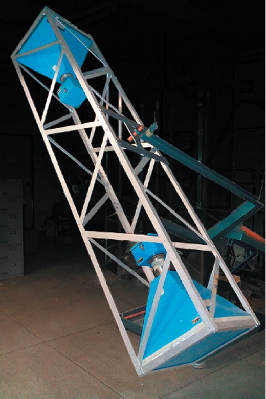
One of the five Tupi telescopes; each one is constituted by two detectors (plastic scintillator 50 cm × 50 cm × 3 cm) within the pyramidal box at the top and bottom positions. On top of each pyramidal box is a (3-inch) photomultiplier. The separation between the detectors is 3 m. (Color online)
Each telescope counts the number of coincident signals in the upper and lower detector. In addition, there is a third detector off the telescope axis in anti-coincidence. The aim of this third detector (not shown in figure 1) is to reject air shower particles produced by high-energy cosmic rays. These events, and other background sources such as thunderbolts and power supply fluctuations, can trigger signals simultaneously in the three detectors.
The output raw data consists of the counting rate of coincidences at 1 Hz versus universal time (UT). The Tupi telescopes are placed inside a building under two flagstones of concrete (150 g cm−2). The flagstones increase the detection muon energy threshold up to ∼ 0.1–0.2 GeV, which is required to penetrate the two flagstones. From a spectral analysis (see subsection 4.2 and figure 9, later), we estimate that that the minimum proton energy at the top of Earth's atmosphere to produce such muons is ∼ 2 GeV. Each Tupi telescope has an effective field of view of ∼ 0.37 sr.
Time synchronization is essential for correlating event data in the Tupi experiment. This is achieved by using the GPS receiver. All steps from signal discrimination to the coincidence and anticoincidence are made via software using the virtual instrument technique. Figure 2 shows the data acquisition system diagram. The application programs were written using the LAB-VIEW tools. The Tupi experiment has a fully independent power supply with autonomy of up to 6 hr to safeguard against local power failures. As a result, the data acquisition is basically carried out with a duty cycle of 95%.
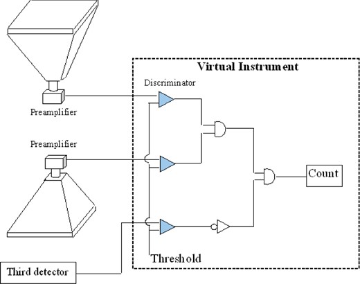
The logic of the data acquisition system of each telescope. It uses the virtual instrument technique within the LabView code. The data acquisition is made at a sample rate of 1 MHz, and the raw data resolution is 1 s. (Color online)
On the other hand, the Earth is surrounded by an almost spherical magnetic field, the magnetosphere, and it is a natural shielding of the Earth's surface to solar and galactic cosmic-ray particles of up to several GeV in energy. On the day side, there is an additional factor linked with the solar wind and its interaction with the magnetosphere that produces a bow shock, shielding the Earth from several types of radiation (charged particles) coming from external space. Due to the compression of the solar wind, the magnetosphere becomes widely asymmetric with a long tail opposite to the Sun. However, at a certain location over the South Atlantic and centred in the south of Brazil, the shielding effect of the magnetosphere is not quite spherical but shows a hole as a result of the eccentric displacement of the center of the magnetic field from the geographical center of the Earth by 280 miles (Fraser-Smith 1987).
This place is the so-called SAA region, and it is the region where the inner Van Allen radiation belt makes its closest approach to the Earth's surface. Figure 3 shows the geographic location of the SAA that is characterized by an anomalously weak geomagnetic field strength (less than 28000 nT) (Barton 1997), and the Tupi telescopes are within this region. This behaviour of the magnetosphere is responsible for several processes, such as the high conductivity of the atmospheric layers due to the precipitation of energetic trapped particles from the inner Van Allen belt. The presence of energetic “trapped” protons above the 50 MeV level shows a 1000-times increase when compared to other regions exterior to the SAA.
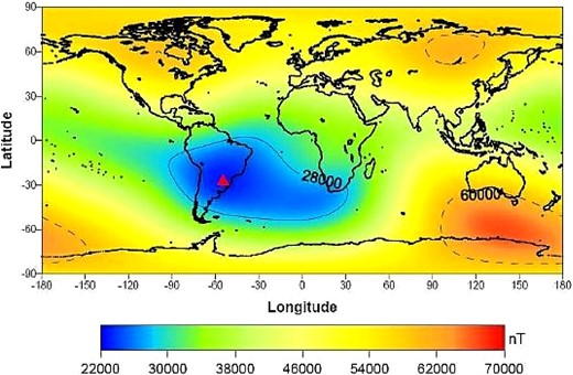
Geographycal distribution (latitude vs. longitude) of the geomagnetic field intensity over the Earth. The South Atlantic Anomaly (SAA) region is limited by the region where the geomagnetic field intensity is less than 2800000 nT. The red triangle indicates the location of the Tupi muon telescopes. (Color online)
In addition, proton flux with energies above 850 MeV in the SAA region is around 10 times the flux out of the SAA region as measured by the HEPAD detector (Boatella et al. 2010). Indeed, the PAMELA collaboration introduced in the SAA area a sub-cutoff in the rigidity (∼ 1.0 GV), which is below the nominal Stormer rigidity cutoff (7–10 GV) (Casolino et al. 2008). According to PAMELA observations, high-rigidity particles are present at all latitudes, whereas lower events (mostly due to protons) are observed only at high latitudes and in the SAA.
3 The muon flux at sea level
Barometric and temperature coefficients for various components of the secondary cosmic rays, such as muons, protons and neutrons, including their dependence on the threshold energy, zenith angle and altitude above sea level, have been obtained via Monte Carlo calculations by means of the CORSIKA code (Kovylyaeva et al. 2013). We have compiled some results of the barometric and temperature coefficients for muons, protons, and neutrons reaching vertically the sea level. They are presented in table 1.
Barometric and temperature coefficients for various secondary particles.*
| Secondary | Barometric coefficient βp, % mbar−1 | ||||
|---|---|---|---|---|---|
| 0.1 GeV | 0.5 GeV | 1.0 GeV | 5.0 GeV | 10 GeV | |
| Muon | −0.16 | −0.14 | −0.12 | −0.06 | −0.04 |
| Proton | −0.84 | −0.86 | −0.88 | −0.74 | −0.70 |
| Neutron | −0.75 | −0.80 | −0.83 | −1.01 | −0.84 |
| Secondary | Temperature coefficient βT, % K−1 | ||||
| 0.1 GeV | 0.5 GeV | 1.0 GeV | 5.0 GeV | 10 GeV | |
| Muon | −0.29 | −0.24 | −0.20 | −0.05 | 0.01 |
| Proton | 7 | −3 | 5 | 3 | −1 |
| Neutron | 9 | −3 | 7 | 9 | −5 |
*All values are obtained at sea level, at vertical incidence, and at several energy thresholds.The results has been obtained using the CORSIKA Monte Carlo code (Kovylyaeva et al. 2013).
The above results reveal that the barometric coefficient for muons at sea level is about seven times lower than the barometric coefficient for the neutron monitors in the low-energy region of interest. In addition, for both muons and nucleons in the low-energy region, the temperature coefficient is smaller than −0.3% K−1 for muons and comparable to zero for the nucleons. In short, the atmospheric variations’ effect, such as the temperature and pressure in the muon flux, can be negligible in a short-term analysis. However, it can be important to long-term variation analysis, covering the annual seasons.
4 The events on April 18
We reported a muon excess, with a significance of up to 3.5% in the Tupi muon telescopes, in association with a radiation storm. Perhaps the anomalous weak magnetic field at the place where the telescopes are installed (SAA central region), together with the low energy threshold of detection (∼ 100 MeV) of a hard (muon) component and the geoeffective condition at Tupi site on 2014 April 18, at the solar blast time, were the best conditions to detect a signal (muon excess) in association with the S1 radiation storm.
We have also found that the energy spectrum of solar protons achieved from the muon excess are in the high-energy (GeV) region, that is, in the tail of the proton energy spectrum obtained by GOES 13.
We also looked for a signal associated with this radiation storm in the NM Data Base (NMDB),3 with positive results in at least four neutron monitors located in the west, relative to the Sun–Earth direction, at the time of solar blast, and still within the geoeffective region. These locations are the South Pole, Newark, Peawanuck, and Mexico. However, the confidence level is up to 3%, which is probably the reason why no alert type was reported for this event on April 18 by the “Real Time GLE ALERT System.” Thus, further investigations are needed to verify if these observations may be considered as a new (GLE) in the current solar cycle. For now, the signal of this event at ground-level detectors is stronger than the three “almost” GLEs indicated above. Details of these observations are reported below.
On 2014 April 18, the solar active region, AR2036, erupted a moderate M7.3-class solar flare with onset at 12:31 UT and peaking at 13:03 UT. The region AR2036 was in a beta–gamma configuration and located at coordinates S20W34 on the solar disk. This means that it occurred in a geoeffective location. The solar blast hurled a CME into space.
The CME image was registered by LASCO (Large Angle and Spectrometric Coronagraph) C-2 on-board the SOHO spacecraft, and it is available in the CACTus LASCO CME catalog (Robbrecht et al. 2009). The CME was a type II radio burst, with a angular width greater than 90°, as shown in figure 4 (left-hand panel). The median velocity of the CME shocks was 812 ± 110 km s−1, and their principal angle was 194° (measured counterclockwise from north). However, the fastest CME shocks, with velocities up to 1008 km s−1, were close to the ecliptic plane; that is, their principal angles were close to 90°.
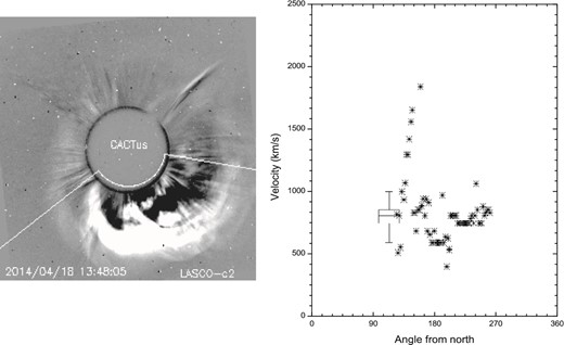
Left-hand panel: Lasco C2 image of the CME on 2014 April 18 at 13:48:05 UT. The angular width of the CME was 134° with a duration of liftoff of 2 hr. Right-hand panel: Velocity distribution of the CME-associated shocks, as a function of the principal angle counterclockwise from north (degrees) (Robbrecht et al. 2009).
We believe that the particles accelerated by these few, but fast, shocks, close to the ecliptic plane, were the origin of the radiation storm observed by GOES, as well being the origin of the particle enhancement observed at some ground-level detectors. The solar, energetic particles began arriving on Earth at 13:30 UT, peaking at an S1-level condition of a radiation storm after two hours.
In addition, according to a NOAA space weather message, a 10-cm radio burst was associated with the event that had its onset at 12:55 UTC. Consequently, it was in association with the M7.3-class eruption. In general, radio emissions are typically associated with strong CMEs and solar radiation storms.
In coincidence with the onset of the solar energetic particles (radiation storm) observed by GOES13, we have found a muon excess with a significance of up to 3.5%. The muon excess was extended beyond 23 UT, with a total duration of 9.6 hr, as shown in figure 5. The figure includes also the X-ray prompt emission according to GOES15 (top panel). The dark area shows the coincidence between the onset of the radiation storm and the fast rise in the muon counting rate as well as the duration of the muon enhancement at the south 45° telescope.
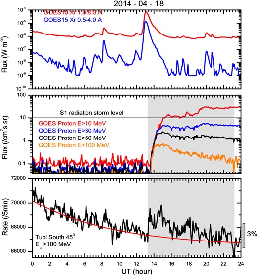
Time profiles on 2014 April 18, in three different detectors. Top panel: the GOES 15 X-ray flux; central panel: the GOES proton flux in four channels (10 MeV, 30 MeV, 50 MeV, and 100 MeV), showing the S1-class radiation storm; bottom panel: the muon counting rate at the southern Tupi telescope. The dark area shows the coincidence between the onset of the radiation storm and the fast rise in the muon counting rate, as well as the duration of the muon enhancement above background, marked by the red curve. (Color online)
On 2014 April 18, at the time of solar blast, the location of Tupi telescopes had the best geoeffective condition as shown in figure 6, where the ionospheric D-Region Absorption Map, is presented. The figure shows the geographical coordinates (latitude vs. longitude) of ground-based detectors: Mexico NM, Newark NM, Peawanuck NM, South Pole NM, and Tupi telescopes, including the nominal sunward positions at 13:14 UT on 2014 April 18. We can see in this figure that the zenith at the location of the Tupi telescopes makes an angle of 38° relative to the Sun–Earth line, which is close to the best condition of 45°. Under this condition, the particles arrive at the Earth with a small pitch angle (pitch angle is the angle between the Sun-ward magnetic field direction and the viewing direction of the telescope or directional channel). We claim that this favorable condition has allowed the registration of a fast rising in the counting rate in the muon telescopes in temporal coincidence with the onset of the radiation storm, as shown in figure 5.
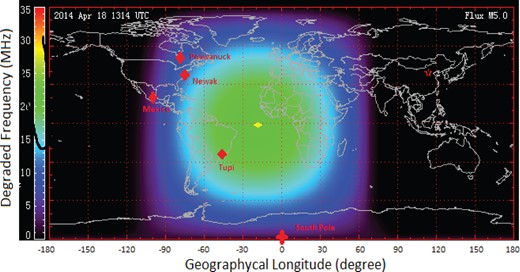
Geographical coordinates (latitude vs. longitude) of ground-based detectors: Mexico NM, Newark NM, Peawanuck NM, South Pole NM, and Tupi telescopes, including the nominal sunward positions at 13:14 UT on 2014 April 18. The colored circles represent the ionospheric D-Region Absorption Map, produced by the Space Weather Prediction Center (SWPC). (Color online)
The next step was to find the signal on the network of cosmic ray stations, NMDB.4 It consists of 36 NM stations; of those, 16 have online data. Indeed, we have found a signal only in those ground-based detectors located at the west relative to the Sun–Earth direction (see figure 6), that is, still within the geoeffective region. We have found an intensity increase in at least four NMs, but their confidences are small, up to 3%, as shown in figure 7. Notice that these NMs are located on American continents, that is, they have relatively similar geographical longitudes. In addition, the particle enhancement at the Mexico NM is smaller. This behaviour is due its high geomagnetic rigidity cutoff at 8.2 GV. The exception is the South Pole NM. However, it has a strategic location, at the South Pole, at latitude −90°, and it is the detector with the lowest geomagnetic rigidity cutoff (0.1 MV) on Earth.
We claimed that the fast rise observed only in Tupi data was originated by protons, accelerated by the flare to relativistic energies, that is, during the impulsive phase of flare. In some flares the timing of electromagnetic emissions and relativistic protons suggests that the first proton peak is related to the acceleration during the impulsive phase (Murphy et al. 1987) by small-scale coronal loops (Pallavicini et al. 1977). A fraction of these high-energy particles can interact with the nuclei of the different elements in the solar atmosphere environment, leading to the production of neutral pions that decay immediately and generate a broad gamma-ray line in the MeV energy range (Kurt et al. 2013).
In this phase there is also the emission of hard X-rays, due to bremsstrahlung produced by electrons that have been accelerated to much higher energies than those found in the ambient plasma (Lin et al. 2003). The hard X-rays and the gamma-ray emissions are the evidence of acceleration of electrons and protons (ions) to relativistic energies in this impulsive phase. We show that this happened in this case since there is a narrow gamma-ray peak, just at the beginning of flare observed by the Fermi Gamma-ray Space Telescope. It is almost in temporal coincidence with the fast rise of the muon count rate at Tupi, as shown in figure 8. Particles accelerated in this impulsive phase are characterized by a fast rise and short decay times. Thus, the impulsive phase has only a duration of some tens of minutes and varies from flare to flare (Pallavicini et al. 1977).
In general, the impulsive phase duration coincides with the rise time of the soft X-rays. In the present case, according to the GOES 15 data (see figure 5, top panel), the time is not longer than 20 min, which is close to the duration of the hard X-ray emission observed by the Fermi (see figure 8).
However, the signal at Tupi extends for more than 9 hr, as indicated by the dark area in figure 5. This means that the signal at Tupi was originated by two populations of solar protons, a very small contribution from those accelerated during the short impulsive phase (less than 20 min), and the main contribution from those accelerated during the gradual phase by CME shocks. The gradual phase is characterized by a soft rise and a long decay time. Thus this gradual phase has a long duration.
It is important to point out that the data shown in figures 5 and 7 suggests that the SEP observed by GOES satellite, as well as the particle enhancement observed in NMs, correlates only with the gradual phase of the solar flare. In short, the duration of the particle enhancements at NMs is approximately 6 hr. However, the total duration observed in the Tupi was longer, 9.6 hr.
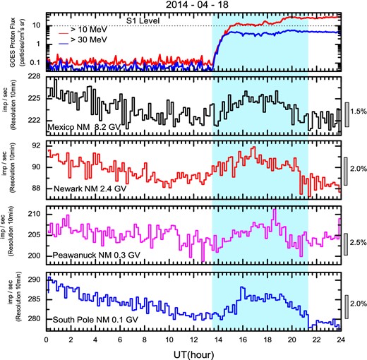
Time profiles on 2014 April 18 showing the solar transient event, in four different detectors. Top panel: the GOES proton flux, showing the S1-class radiation storm. Second, third, and fourth panels: the particle counting rate in the Mexico NM (8.2 GV), Newark NM (2.4 GV), and Peawanuck NM (0.3 GV). The light blue area shows the coincidence between the onset of the radiation storm, almost coincident with the rise in the particle counting rate up to its end, that is, the duration of the particles’ enhancement. (Color online)
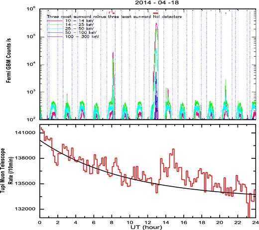
Time profiles on 2014 April 18, from two different detectors. Top panel: the Fermi Gamma-ray Space Telescope counting rate in five channels of energy. Bottom panel: the muon counting rate at the southern Tupi telescope. The curve shows the muon excess above background. (Color online)
We would like to point out that an automatic GLE Alarm has been developed using the eight Bartol NMs stations (Kuwabara et al. 2006). Automated e-mail alarms can be sent to subscribers within minutes of large GLE onsets. Similarly, there is the Real-Time GLE ALERT System developed by the National and Kapodistrian University of Athens-Cosmic Ray Group which uses the ESA NM stations (Souvatzoglou et al. 2009).5
Both systems use the same scale: the systems generate a QUIET (or alert level 0) when no station observes an increase, a WATCH (or alert level 1) when one station observes an increase of 4% or more in a 3-min moving average, a WARNING (or alert level 2) when two stations observe such an increase, and an ALERT (or alert level 3) when three or more stations record such an increase. On April 18, no alert level 3 (ALERT) was reported. However, perhaps the small confidence of up to 3% was the reason why no alert was reported.
5 Results of spectral analysis
The convolution is between the yield function S(Ep) (the number of muons at sea level per incident proton) obtained from Monte Carlo simulation (Poirier & D'Andrea 2002) and the energy spectrum, Np(Ep), given by equation (2). The specific yield function as a function of proton energy is determined using FLUKA,6 which is a detailed general purpose tool for calculations of particle transport and interactions with matter. The result seen in Poirier and D'Andres (2002) does not take into account the geomagnetic rigidity cutoff. This FLUKA output is shown as solid squares in figure 9.
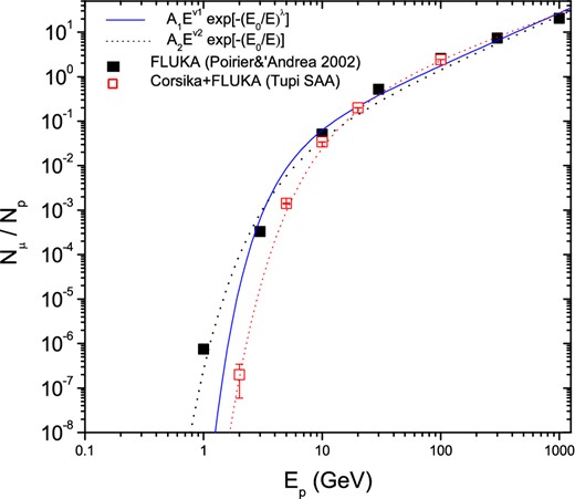
Yield function, as the number of muons at the sea level per proton (vertical incidence), as a function of incident proton energy, from FLUKA calculations (black squares) (Poirier & D'Andrea 2002) and from CORSIKA-FLUKA, taking into account the SAA's magnetic conditions. The curves show several fit functions. (Color online)
We have also included results of our own simulation using FLUKA within CORSIKA, taking into account the geomagnetic conditions of the Tupi's location, close to the central region of the SAA. CORSIKA (COsmic Ray SImulations for KAscade)7 is a physics computer software for simulation of air showers; we choose the compile option FLUKA to describe the hadronic interaction.
In the FLUKA-CORSIKA option, the geomagnetic field effect is taken into account in two different stages of the simulation chain. The first takes into account only the local geomagnetic field during shower development in the atmosphere. This is useful when the primary particle is neutral, such as a gamma-ray (Augusto et al. 2015). The second, and more important for our objectives, takes into account the geomagnetic rigidity cutoff on the primary particle through the magnetic deflection at a given location (point of first interaction). The effect of geomagnetic cutoff modulates the primary spectrum because, at a given location and for a given direction, a threshold in magnetic rigidity exists. The magnetic parameters of the Tupi site are summarized in table 2.
Geomagnetic parameters of the Tupi place analysed here.
| Site | B (horizontal) | B (vertical) | Stormer vertical |
|---|---|---|---|
| (mT) | (mT) | rigidity cutoff (GV) | |
| Tupi | 18.13 | −16.60 | 9.2 |
| Site | B (horizontal) | B (vertical) | Stormer vertical |
|---|---|---|---|
| (mT) | (mT) | rigidity cutoff (GV) | |
| Tupi | 18.13 | −16.60 | 9.2 |
To vertical incidence of charged particles, the horizontal component of the magnetic field defines the vertical geomagnetic rigidity cutoff. Basically only the polar regions have a B (horizontal) component smaller than that of Tupi's location. This is the origin of the sub-cutoff on the geomagnetic rigidity observed in the SAA region.
The convolution between the yield function, S (Ep), and the particle spectrum Np (Ep) gives the response function, which is the number of muons in the excess generated by the SEP during a period T.
In order to compare it with the flow of SEP observed by GOES, the proton flow in the high-energy tail is estimated in a period T = 5 min and corresponds at the peak of the muon count rate with a resolution of 5 min (see figure 5). The peak at Tupi happens at 14:50 UTC, that is, 1.52 hr after the onset. Thus, according to the analysis presented in section 4, the peak of the muon excess at Tupi can be linked with the gradual phase of the flare.
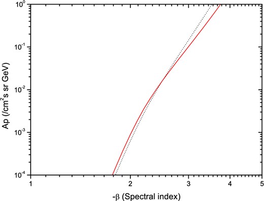
Correlation between the coefficient Ap and the spectral index β. All possible values of Ap and β compatible with the observed muon flux (dot line) and the integrated fluence F (solid line) are obtained on the basis of Monte Carlo simulations and analytical calculations. These quantities are defined by equations (3) and (5). (Color online)
All possible values of β and Ap compatible with this muon fluence are represented by the solid line in figure 10. Thus, one can obtain the best estimate for the spectral index β and Ap using the intersection of two curves defined by equations (3) and (5).

Integral proton flux: the blue triangles and the red circles represent the GOES 13 data, and correspond to the proton flux background and when the radiation storm reaches the level S1 on 2014 April 18, respectively. The black squares represent the proton flux obtained from the muon excess on the Tupi telescope, observed in coincidence with the radiation storm. (Color online)
The origin of this transient event was the solar eruption, an M7.3-class flare and its associated CME, accelerating protons (ions) up to relativistic energies beyond the GeV energies. However, the flux was only strong enough to be considered as an S1 (minor) radiation storm.
6 Conclusions
The shielding effect of the magnetosphere is lowest in the SAA region, and the Tupi muon telescopes are within it and close to its central region. We found that this characteriztic is useful for the observation of solar transient events through their effects at the ground level as well as at sea level. In this paper, we have presented ground-based observations and particle excess linked with a radiation storm on April 18 following the M7.3-class flare and their associated CME from the active region AR2036 to the west of the solar disc. The blast has accelerated protons (ions) reaching up to a value required to be considered a radiation storm (S1), according to the NOAA storm scale.
We claim that such a radiation storm has a GeV component and it might have triggered a new ground-level enhancement (GLE) in the current solar cycle, because a fast rise in the muon counting rate has been observed, in coincidence with the onset of the S1 radiation storm. The signal at the Tupi telescope has a significance of up to 3.5% at peak and the muon excess remained above the background for approximately 9.6 hr. We would like point out that at the time of the blast Tupi had the best geoeffective location relative to the other ground-level detectors.
In addition, a gradual increase in the particle intensity was found in at least four neutron monitors provided by the neutron monitor database (NMDB) network. They are located at the South Pole, Newark, Peawanuck, and Mexico. However, their confidences are small: up to 3%. Perhaps this is the reason why no alert type was reported by the “Real-Time GLE ALERT System.” Note that basically there is signal only in ground-based detectors located at the west relative to the Sun–Earth direction (see figure 6), that is, within the geoeffective region.
The different behaviours observed between the muon detector and the NMs can be linked with the different particle species observed by these two detectors. The muon component of the cosmic rays is known as the hard component due to the their large penetration. Thus, the signal at muon detectors can be linked with the the maximum flare energy release during the impulsive phase of the flare (duration no longer than 20 min). It overlaps with a gradual phase that has a duration greater than 9 hr. The observation of this gradual phase at NMs and Tupi suggests that it is linked with the magnetic restructuring in the corona after the CME passage, and indicates the gradual phase of the solar flare and acceleration of protons (ions) by CME shock waves.
We acknowledge the Space Weather Prediction Center (SWPC); the Fermi Solar Flare X-Ray and Gamma-Ray Observations; the CACTus COR2 CME list and the NMDB database,8 founded under the European Union's FP7 programme (contract No. 213007) for providing data. The neutron monitors at Peawanuck and the South Pole are provided by the University of Delaware Department of Physics and Astronomy and the Bartol Research Institute. This work is supported by Fundação de Amparo a Pesquisa do Estado do Rio de Janeiro (FAPERJ), under Grant 08458.009577/2011-81 and E-26/101.649/2011.
FLUKA (“FLUktuierende KAskade”) 〈http://www.fluka.org/fluka.php〉.
References
