


Abstract
The coronavirus disease (COVID-19) represents a large increase in background risk for individuals. Like the COVID-19 pandemic, extreme events (e.g. financial downturns, natural disasters, and war) have been shown to change attitudes towards risk. Using a risk apportionment approach, we examine whether risk aversion as well as higher order risk attitudes (HORAs) (prudence and temperance) have changed during COVID-19. This methodology allows us to measure model-free HORAs. We include prudence and temperance as higher order measures, as these two have been largely understudied under extreme events but are determinants of decisions related to the health and financial domains. Once we account for socio-demographic characteristics, we find an overall increase in risk aversion during COVID-19. We also find similar results using a hypothetical survey question which measures willingness to take risks. We do not find changes in prudence and temperance using the risk apportionment methodology.
1. Introduction
Individual preferences, including attitudes towards risk, can change as a result of extreme events like natural disasters, economic recessions, or war and conflict.1 The current coronavirus disease (COVID-19) pandemic is one such large-scale extreme event, which can affect risk attitudes through two key channels. First, it has disrupted economic activity, which has previously been shown to make individuals more risk averse (Shigeoka, 2019). Second, COVID-19 currently represents an additional and large increase in background risk for individuals (background risks are those risks that are not under the control of the agents and are independent of other endogenous risks, Eeckhoudt et al., 1996). Theoretical work on expected utility (EU) maximization shows that an increase in background risk leads to an increase in risk aversion (Kimball, 1993; Gollier and Pratt, 1996). The empirical evidence also identifies a positive relationship between background risk and risk averse behaviour (Hanaoka et al., 2018).
Although the effect of extreme events on risk aversion (dislike for variance) has been previously studied, their impact on higher order risk attitudes (HORA) such as prudence (preference for positive skew) and temperance (dislike for positive kurtosis) remain unexamined (Trautmann and van de Kuilen, 2018). In this paper, we elicit risk aversion, prudence, and temperance before and after the pandemic and examine if there are changes in individual attitudes. For this study, we use the risk apportionment method of Eeckhoudt and Schlesinger (2006) in an online experiment to measure HORA. We also compare responses to the self-reported question of Dohmen et al. (2011) which has been extensively used to measure willingness to take risks (Charness et al., 2013). To the best of our knowledge, this is the first study to evaluate changes in HORA after an extreme health-related event.
Exploring the effect of COVID-19 on HORA is important from both a policy and academic perspective. For policy-makers, learning about HORA is crucial because they play a significant role in decisions pertaining to precautionary savings, insurance choices, financial investments, occupational choices, and health behaviours (Noussair et al., 2014; Decker and Schmitz, 2016; Heinrich and Mayrhofer, 2018). All these aspects of life have been affected by the pandemic. More directly related to COVID-19, risk attitudes impact preventative health behaviour and the take-up of a potential vaccine against the disease (Courbage and Rey, 2006; Mayrhofer and Schmitz, 2020). In addition, assumptions about risk attitudes are central to economic theory, thus it is crucial to know whether risk attitudes are stable or not as they directly affect decision-making.
Overall, once we control for demographic characteristics, we find an increase in risk averse choices during COVID-19 for both incentivized (risk apportionment) and hypothetical (self-reported) questions. However, the increase is heterogeneous across demographics. Prudence and temperance are not significantly different before and after the onset of COVID-19. More specifically, we find that risk aversion increases for all income levels, but lower income individuals have a smaller increase compared with higher income individuals. Our analysis suggests that financial assistance received by lower income workers in the form of additional unemployment insurance could be driving this result as this assistance increased their overall income during the first months of the pandemic.
Our paper contributes to several strands of literature. First, to the literature on measuring individual risk attitudes during COVID-19. Examples of this expanding literature include Li et al. (2020) and Shachat et al. (2020), who find that there is an increase in risk aversion using incentivized Holt and Laury (2002) tasks in Chinese samples. Angrisani et al. (2020) use the Bomb Risk Elicitation Task (Crosetto and Filippin, 2013) and find no average effect of COVID-19 on risk attitudes for portfolio managers and students. However, they do find that those subjects who were diagnosed with COVID-19 became more risk averse. In our paper, we go beyond risk-aversion by providing measures of HORA (prudence and temperance) that are model-free.
Second, we contribute to the literature on how risk attitudes change after extreme events (Eckel et al., 2009), by examining changes in behaviour after a large economic and health shock. Third, our paper adds to the growing literature on measuring HORA (Trautmann and van de Kuilen, 2018; Schneider and Sutter, 2020) as we measure not only risk aversion but also prudence and temperance. Last, we contribute to the literature comparing incentivized risk elicitation tasks to hypothetical ones (Anderson and Mellor, 2009), by comparing risk aversion measured through a lottery-based method against a hypothetical willingness to take risks question.
The rest of the paper is structured as follows: Section 2 presents the experimental design, Section 3 discusses our results, and Section 4 is the concluding section.
2. Experimental design
The experiment consists of a single stage where we elicit HORA. The intervention was at the onset of COVID and we compare HORA-elicited pre-COVID (April and May 2018) and post-COVID (May 2020). Section 2.1 is adapted from Mussio and de Oliveira (2021). The experiment is followed by a questionnaire.
2.1 HORA elicitation
We elicit HORA using the risk apportionment method of Eeckhoudt and Schlesinger (2006) and Eeckhoudt et al. (2009). This is an experimental approach which uses 50–50 lottery pairs to define risk aversion, prudence, and temperance (Eeckhoudt et al., 2009; Crainich et al., 2013) and allows us to link observable choices to unobservable properties of the utility function.
2.1.1 Risk apportionment methodology
Consider an individual with wealth,
Risk aversion under the Eeckhoudt and Schlesinger (2006) approach is defined as a preference for disaggregating two potential changes in wealth across two equally likely states of nature. Figure 1(a) shows the generic lottery pairs used to elicit risk aversion. Lottery A2 has a 50% chance of W and a 50% chance of
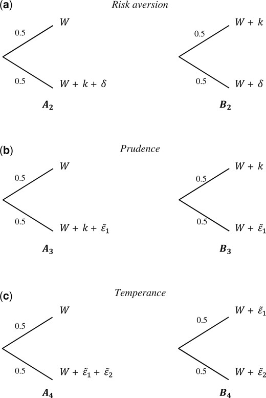
Lottery pairs for (a) risk aversion, (b) prudence, and (c) temperance tasks.
Notes: W, k, and δ represent fixed amounts while
Under this methodology, prudence is defined as a preference for disaggregating zero-mean risks and a sure change in wealth across two equally likely states of nature. Consider the generic lottery pairs to measure prudence shown in Fig. 1(b). Lottery A3 has a 50% chance of
Lastly, temperance is a preference for disaggregating two independent zero-mean risks across two equally likely states of nature (Ebert and Wiesen, 2014). The general form for the temperance choice tasks is shown in Fig. 1(c). Consider lottery A4, which has a 50% chance of
2.1.2 Description of the choice tasks and format
Eliciting HORAs is a complex task regardless of the methodology used. This is particularly the case once orders higher than temperance are reached. In our experiment, participants make their decisions following the format proposed by Deck and Schlesinger (2010) and previously used by Mussio and de Oliveira (2021). The layout of Deck and Schlesinger (2010) allows participants to make two simultaneous decisions in each task in a simplified and intuitive manner (with the decisions being based on a single coin toss).2 The format makes the choice of whether to aggregate or disaggregate events explicit and easy to understand.
When items are fixed dollar amounts, they are presented to the participants as [x/x] (Deck and Schlesinger, 2010). When items are for zero-mean lotteries, they are presented as [x/−x], where x is the amount that can be won or lost. Columns 3 and 4 of Table 1 have examples of both formats. A screenshot of how decisions and choices are set up for the participant can be found in the Online Appendix A.
HORA elicitation—risk choice tasks
| Decision | Endowment (W) | First item | Second item | Expected payoff |
|---|---|---|---|---|
| 1-R | 10 | [1/1] | [1/1] | 11 |
| 2-R | 10 | [1/1] | [5/5] | 13 |
| 3-R | 10 | [1/1] | [9/9] | 15 |
| 4-R | 10 | [5/5] | [5/5] | 15 |
| 5-R | 6 | [9/9] | [9/9] | 15 |
| 6-R | 50 | [5/5] | [45/45] | 75 |
| 7-P | 30 | [25/25] | [25/−25] | 42.5 |
| 8-P | 12.5 | [9/9] | [5/−5] | 17 |
| 9-P | 12.5 | [1/1] | [5/−5] | 13 |
| 10-P | 10.5 | [9/9] | [1/−1] | 15 |
| 11-P | 12.5 | [5/5] | [5/−5] | 15 |
| 12-P | 14.5 | [1/1] | [9/−9] | 15 |
| 13-T | 15 | [5/−5] | [5/−5] | 15 |
| 14-T | 15 | [9/−9] | [1/−1] | 15 |
| 15-T | 55 | [25/−25] | [25/−25] | 55 |
| 16-T | 55 | [5/−5] | [45/−45] | 55 |
Notes: [x/x] denotes a sure amount of E$x. [x/−x] represents a 50/50 lottery with the amounts specified in brackets. In Column 1, -R represents a risk aversion task, -P represents a prudence task, and -T a temperance task.
Source: Choice tasks determined by authors based on Deck and Schlesinger (2010).
Table 1 presents the 16 choice tasks to measure risk aversion, prudence, and temperance which are presented to the subjects in a randomized order. All amounts are defined in terms of experimental dollars (E$). The conversion rate was set at E$80 equal to US$1. Participants start with a fixed amount of money (
Participants make their decisions following the format described next. When items are fixed dollar amounts, they are presented to the participants as
Below are two examples of tasks the participant sees. First, we present the following example of a risk aversion task (items for this example task are listed as task 3 in Table 1) which is presented in the format of Deck and Schlesinger (2010):
You will receive E$10 +
[1/1] if the coin lands on Heads or Tails and
[9/9] if the coin lands on Same or Different outcome.
In this choice task, the participant starts with a fixed amount of E$10. As an example of a risk averse participant, suppose the participant selects Tails and Different, thus preferring lottery B2. A risk averse participant would choose Different, corresponding to B2, preferring to disaggregate the outcomes. If the coin toss lands on tails, the participant receives $11 with certainty. If it lands on heads, the participant receives E$19. As an example of a risk seeking participant, suppose they choose Heads and Same, thus preferring lottery A2. If the coin lands on heads, the participant receives E$20. If the coin flip lands on tails, the participant only receives the fixed amount, E$10.
In addition, the participant will also see the following task to measure prudence (items for this example task are listed as task 12 in Table 1):
You will receive E$14.50 +
[1/1] if the coin lands on Heads or Tails and
[9/−9] if the coin lands on Same or Different outcome.
In this choice task, the participant starts with a fixed amount of E$14.50. As an example of a prudent participant, suppose the participant selects Tails and Different, thus preferring lottery B3. A prudent participant would choose Different, corresponding to B3, preferring to disaggregate the outcomes. If the coin toss lands on tails, the participant receives $15.50 with certainty. If it lands on heads, the participant receives either E$23.50 or E$5.50, with a 50% probability each. As an example of an imprudent participant, suppose they choose Heads and Same, thus preferring lottery A3. If the coin lands on heads, the participant receives either E$24.50 or E$6.50, with a 50% probability each. If the coin flip lands on tails, the participant only receives the fixed amount, E$14.50.
2.2 Socio economic and COVID-19 questionnaires
After the HORA elicitation, individuals completed a questionnaire. The first block of questions includes questions regarding beliefs, attitudes, and behaviours during COVID-19. This block is shown to the during-COVID sample only and its main objective is to ensure that participants comprehend the nature of COVID-19.3
The second block of questions gathers data on participants’ background risks, including health risks, employment and labour income, liquidity constraints, and risky behaviours (Cardak and Wilkins, 2009; Noussair et al., 2014). The third block of questions is a socioeconomic survey, which includes, among other questions: age, gender, state of residence, and marital status, as well as a self-reported risk aversion question à la Dohmen et al. (2011). The two last questionnaire blocks are common to both sub-samples (pre- and during-COVID). The questionnaire and summary of responses from the COVID-19 questions are available in the Online Appendix B.
2.3 Implementation and payment
Our experiment was conducted online. It was programmed in Qualtrics and subjects were recruited from Amazon Mechanical Turk (MTurk). The first stage of the experiment took place in April and May 2018, where we collected HORA elicitations for 1,105 participants in the USA (18 years or older). The data collection during COVID-19 took place in May 2020 (during COVID-19) and we collected data for 322 participants.
During the experiment, the participants watched a video with instructions. This video included both oral and visual descriptions of how the tasks worked, as well as examples of how to calculate outcomes based on the coin toss and individual choices. This was followed by comprehension questions including an example of a task to calculate potential payments and a captcha button to screen out bots. We used two comprehension questions which allowed subjects to test their knowledge about the experiment and in which the answers varied in terms of the head versus tails and same versus different choice selection for outcome calculation (see the detailed comprehension questions and full script of the instructions video in the Online Appendix D). The comprehension questions were used for screening purposes, as participants were only allowed to move on to the experiment if they answered these questions correctly. To avoid negative earnings, participants started with an endowment of 100 experimental dollars (E$). Each individual experimental session lasted around 20–25 min and participants were paid right after the session was finished. The 2020 experimental protocol was identical to the 2018 one except for the inclusion of COVID-19-related questions.
Payment for the experiment is based on individual decisions in the tasks presented in Section 2.1 and includes the outcome of one of their experimental tasks, which is randomly selected. The exchange rate for the outcome of the experimental task was E$80:$1. The average MTurk payment in 2018 was $1.06 (st.dv. $0.54) and for the 2020 COVID-19 data collection wave was $0.42 (st.dv. $0.34), in addition to the fee earned for entering the experiment in MTurk (HIT).
In 2020, we paid participants $10 for entering the HIT while the 2018 experiment was part of a bigger data collection process and participants received $0.50 for entering the HIT. The increase in HIT was to speed up the process of subjects signing up for the experiment, given the time sensitive nature of our data collection. The changing of the fee raises two possible concerns. First, it may have a selection effect where the participants who sign up for the experiment are different. We addressed selection concerns by checking for sample balance on both waves. We also use a matching procedure to control for differences between samples, described in Section 3. Second, it may change behaviour of participants due to different background wealth. However, this fee is independent of the experiment and prior research shows that HIT values do not change the outcome of experiments (Andersen and Lau, 2018). We also control for differences in background wealth in our analysis.
3. Results
We first examine whether our sample was affected by COVID-19. We then present effects of the pandemic on HORA. Finally, we analyse the responses to the general hypothetical risk question (Dohmen et al., 2011).
3.1 Understanding of COVID-19 and its impact on the sample
By the end of April 2020 (the week prior to the start of the experiment) almost one million COVID-19 cases and over 74 thousand COVID-19-related deaths were declared in the USA by the Centers for Disease Control and Prevention (2020). In total, 33% of our sample knew someone (including themselves) who tested positive for COVID-19. This is a higher number compared with survey samples in other countries such as China, where about 2.3% stated the same (Yue et al., 2020). COVID-19 represents an increase in background risk as it is exogenous but is also a change in uncertainty, as there is lack of control, catastrophic potential, and changes in risk perception, influenced by the media and the public in general and sustained by the ubiquity of negative events, such as deaths and contagion (Slovic, 2010; Aven and Bouder, 2020). If people understand the severity of the pandemic, we should see an impact on their behaviour. Therefore, in a first stage of our analysis, we briefly examine the responses to survey questions related to COVID-19.
First, a large proportion of participants has an understanding of the basic clinical aspects of COVID-19, such as the main symptoms (87%), who is at risk of developing a severe case of the illness (65%) and how the virus can pass even through people who are asymptomatic (84%). The risk that our results are impacted by lack of comprehension of COVID-19 seems therefore limited. In addition, the onset of COVID-19 brought a change in everyday behaviours. We find evidence of adaptive health behaviours, as almost 90% of our sample state that their daily behaviours changed, including washing their hands more frequently, avoiding social gatherings, and staying at home (see Table B.2 in Online Appendix).
Many of the responses are also consistent with the predictors of risk perception of COVID-19 found by Dryhurst et al. (2020), which include whether individuals had direct experience with the virus, their trust in the government strategy to tackle the virus and prosocial behaviours. Over 80% of our participants agree that people are following precautions to reduce the spread of the virus. They also report that people around them are facing economic hardship (69%). Only one-third of them agree that the country’s authorities have responded to the COVID-19 pandemic well.
Thus, a significant percentage of our participants understand the basics of contagion and have adopted behaviours to avoid passing on the virus to others indicating that COVID-19 has impacted their lives.
3.2 Treatment effects on HORA
We examine the impact of the COVID pandemic on HORA using a joint estimation, matching the individuals in both the 2018 and 2020 samples. This method accounts for the theoretical relationship between the measures and ensures balanced samples.
The identifying assumption of our estimation is that nothing else of the magnitude of COVID-19 happened between the time period of our samples that can impact our results. To the best of our knowledge, we are not aware of any study arguing for the existence of any other background risk shocks of this size that could impact risk attitudes for all individuals in the USA occurring after our 2018 data collection but before the onset of COVID-19. Moreover, there is no evidence to believe that there are other economic events affecting uncertainty in the magnitude of COVID-19. As pointed out by Baker et al. (2020), the financial volatility recorded in March 2020 was the highest in recent history, including the Great Recession. Similarly, Altig et al. (2020) analysed several measures of economic uncertainty in the USA before and during the pandemic. The authors studied stock market volatility, newspaper-based policy uncertainty, Twitter chatter about economic uncertainty, and macroeconomic forecasting, and show a relative stability in all measures during 2018 and 2019 and record jumps in 2020.
Public opinion is consistent with these findings. In May 2020 (when we collected the data), 9 out of 10 US adults believed that the coronavirus outbreak was a major threat to the US economy (Pew Research Center, 2020). Similarly, almost 70% of our subjects reported that either themselves or someone they knew faced economic hardship because of the pandemic (Table B.1 in Online Appendix B). In summary, while we cannot rule out the presence of other factors affecting risk attitudes, the evidence suggests that the COVID-19 was the most dominant factor.
3.2.1 Matching pre- and during COVID samples
If COVID-19 has an impact on the type of subject who would participate in our experiment, our results could be exposed to a potential source of endogeneity. To minimize the impact of this potential endogeneity, we implement a matching estimation. We use a 1-nearest-neighbor matching method with replacement. For the matching, we include gender, age, income, marital status, education, race and ethnicity, health status, and region in the USA.4 Our nearest neighbour matching method finds matches 312 participants during-COVID and generates samples that are balanced on socio-demographics (see Table 2). We restrict the sample to have 1 match per observation only, with no maximum distance as potential matching (no calipers or exact-matching). All our matching covariates are discrete. For this reason, the Abadie and Imbens (2011) bias correction is not necessary in the case.
Balance tests for socioeconomic matched variables (nearest neighbour)
| Pre-COVID | During COVID | Balance test p-value | |||
|---|---|---|---|---|---|
| Mean | SD | Mean | SD | ||
| Female | 0.45 | 0.50 | 0.43 | 0.50 | 0.69 |
| Age | 36.28 | 10.23 | 38.32 | 11.40 | 0.02 |
| Income | 5.59 | 2.76 | 5.44 | 2.97 | 0.49 |
| Education | 4.55 | 1.21 | 4.58 | 1.29 | 0.77 |
| Health | 4.11 | 0.78 | 3.99 | 0.87 | 0.07 |
| Married | 0.65 | 0.48 | 0.68 | 0.47 | 0.45 |
| Northeast | 0.20 | 0.40 | 0.20 | 0.40 | 1.00 |
| Midwest | 0.36 | 0.48 | 0.36 | 0.48 | 1.00 |
| South | 0.18 | 0.38 | 0.18 | 0.38 | 1.00 |
| Hispanic | 0.20 | 0.40 | 0.21 | 0.41 | 0.77 |
| White | 0.77 | 0.42 | 0.74 | 0.44 | 0.31 |
| Children | 0.57 | 0.50 | 0.58 | 0.49 | 0.69 |
| Home ownership | 0.68 | 0.47 | 0.70 | 0.46 | 0.61 |
| N | 312 | 312 | |||
Source: Authors’ calculations.
Definitions and overall statistics for our explanatory variables can be found in Table 3. With the balanced samples, we calculate average treatment effects on the treated (ATETs) for risk aversion, prudence, and temperance on the balanced sample (Table 4). We find that ATETs are not significant for any of the HORA. We also perform average tests on distribution changes and the number of choices pre- and during COVID. We do not find significant differences in these measures either. Therefore, we conclude that on the average, there are no significant changes to HORA by using incentivized risk apportionment tasks.5
Variable summary
| Variable | Definition | Mean | SD | Min | Max |
|---|---|---|---|---|---|
| Low income | 1 if income is less than $20,000 a year | 0.215 | 0.411 | 0 | 1 |
| Tertiary education | 1 if participant has a complete university degree or higher | 0.709 | 0.454 | 0 | 1 |
| Chronic illness | 1 if participant reports having at least one chronic illness | 0.606 | 0.489 | 0 | 1 |
| Married | 1 if participant reports being married | 0.592 | 0.492 | 0 | 1 |
| Age | Age of the participant, in years | 37.535 | 12.088 | 18 | 89 |
| Northeast | 1 if participant lives in the Northeast region | 0.194 | 0.395 | 0 | 1 |
| Midwest | 1 if participant lives in the Midwest region | 0.381 | 0.486 | 0 | 1 |
| South | 1 if participant lives in the South region | 0.211 | 0.408 | 0 | 1 |
| Hispanic | 1 if participant reports ethnicity as Hispanic or Latino | 0.106 | 0.308 | 0 | 1 |
| Female | 1 if participant reports gender as female | 0.518 | 0.500 | 0 | 1 |
| Black | 1 if participant reports race as Black or African American | 0.082 | 0.275 | 0 | 1 |
| Children | 1 if participant reports having at least one child | 0.516 | 0.500 | 0 | 1 |
| Owns home | 1 if participant reports owning their home | 0.584 | 0.493 | 0 | 1 |
| During COVID | 1 if the participated in the experiment during the COVID-19 pandemic | 0.221 | 0.415 | 0 | 1 |
| N | 1,410 | ||||
Notes: Northeast: Connecticut, Maine, Massachusetts, New Hampshire, Rhode Island, Vermont, New Jersey, New York, and Pennsylvania. South: Delaware, Maryland, Virginia, West Virginia, Alabama, Florida, Georgia, Kentucky, Mississippi, North Carolina, South Carolina, Tennessee, Oklahoma, Texas, Arkansas, and Louisiana. Midwest: Illinois, Indiana, Michigan, Minnesota, Ohio, Wisconsin, Iowa, Kansas, Missouri, Nebraska, North Dakota, and South Dakota. Omitted is West: includes Colorado, Montana, Utah, Wyoming, New Mexico, Arizona, California, Hawaii, Nevada, Alaska, Idaho, Oregon, and Washington (United States Census Bureau, 2010).
Source: Authors’ calculations.
Average treatment effects, mean, and distribution tests for HORA
| Average treatment effect (nearest neighbour) | Average number of decisions pre-COVID | Average number of decisions during-COVID | Means test pre versus during (t) | Wilcoxon test of equality of distributions (z) | |
|---|---|---|---|---|---|
| Risk aversion | −0.002 (0.158) | 2.857 (1.920) | 2.705 (1.968) | 1.226 [0.220] | 1.425 [0.154] |
| Prudence | 0.032 (0.140) | 2.918 (1.835) | 2.923 (1.753) | −0.035 [0.972] | −0.298 [0.766] |
| Temperance | −0.013 (0.104) | 1.971 (1.355) | 1.968 (1.368) | 0.033 [0.973] | 0.022 [0.983] |
| N | 1,098 | 312 | |||
Notes: Average treatment effect is calculated with a nearest-neighbour matching method, using a Mahalanobis distance metric. Standard deviation between parentheses, p-values between brackets for mean equality tests. Number of decisions, means tests, and Wilcoxon tests are performed on the matched sample. Number of risk averse decisions: Min = 0 and Max = 6; number of prudent decisions: Min = 0 and Max = 6; and number of temperate decisions: Min = 0 and Max = 4.
Source: Authors’ calculations.
3.2.2 Joint estimation of the impact of HORA and heterogeneous effects
Although HORA are related theoretically, the ATEs overlook the relationship between the measures by focusing on effects that are independent from each other. The ATE measurement also has the drawback that we could be overlooking heterogeneous effects of COVID-19 on HORA across demographic characteristics. To address these two issues, the theoretical correlation between HORA and the heterogeneous impact of COVID-19 as a background risk, we jointly estimate the impact of COVID-19 on the number of risk averse, prudent, and temperate choices. We specify our model as a three-equation, seemingly unrelated regression (SURE) model (Zellner and Theil, 1962). Each equation in the system is specified as an ordered logit. The model is estimated using a conditional mixed process framework with a maximum-likelihood procedure (Roodman, 2011). To account for heterogeneous effects, we include interaction terms. We interact our measure for COVID-19 with gender, income, health status, as well as race and ethnicity.
In Table 5 (Specification 1), the results from our model show that there is an heterogeneous impact of COVID on risk aversion. An increase in background risk (as proxied by COVID-19) leads to a higher number of risk averse choices in our reference group (high-income, healthy, and white males). There is also a significant but smaller increase in risk averse choices for low-income individuals, as seen by the negative coefficient in the interaction term.
Estimation results of HORA and non-incentivized risk question
| (1)Joint estimation of HORA | (2)Risk question à la Dohmen etal. (2011) | |||
|---|---|---|---|---|
| Number of risk averse choices | Number of prudent choices | Number of temperate choices | Willingness to take risks | |
| During COVID | 0.571*** | 0.249 | 0.142 | 0.389** |
| (0.175) | (0.173) | (0.177) | (0.182) | |
| During COVID * Female | −0.272* | −0.006 | −0.063 | 0.111 |
| (0.140) | (0.138) | (0.141) | (0.136) | |
| During COVID * Low income | −0.053** | −0.025 | 0.002 | −0.076*** |
| (0.022) | (0.021) | (0.022) | (0.025) | |
| During COVID * Health | −0.272* | −0.182 | −0.189 | −0.174 |
| (0.140) | (0.139) | (0.142) | (0.143) | |
| During COVID * Black | −0.249 | −0.221 | −0.093 | −0.066 |
| (0.221) | (0.219) | (0.224) | (0.231) | |
| During COVID * Hispanic | −0.382* | −0.039 | 0.027 | −0.263 |
| (0.202) | (0.200) | (0.205) | (0.229) | |
| Atanrho risk aversion/prudence | 0.647** | |||
| (0.031) | ||||
| Atanrho risk aversion/temperance | 0.419** | |||
| (0.031) | ||||
| Atanrho prudence/temperance | 0.710** | |||
| (0.031) | ||||
| Socioeconomic controls | Yes | Yes | Yes | Yes |
| Likelihood ratio test | 102.70 | 160.23 | ||
| N | 1,410 | 1,408 | ||
Notes: Specification (1): joint estimation of HORA, SURE model. ***p < 0.01, **p < 0.05, *p < 0.1. Atanrho coefficients represent the transformed (arc-tangent), unbounded correlation coefficient of a pair of equations (Roodman, 2011). Specification (2): ordered probit estimation of the individual response to the risk taking variable ‘How do you see yourself: are you generally a person who is fully prepared to take risks or do you try to avoid taking risks?’. Takes the value 1 if ‘very willing to take risks’ and the value 10 if ‘not at all willing to take risks’. Coefficients are presented as log-odds. Robust standard errors in parentheses. Socioeconomic controls include the variables Table 3: (low) income, education, health, marital status, age, regions in the USA, gender, race and ethnicity, children in the household, home ownership, and credit card ownership.
Source: Authors’ calculations.
Compared with pre-COVID measures, we find that there is an overall higher likelihood of making a more extreme number of risk averse choices (four to six choices) during-COVID (Fig. 2). There is also a comparative reduction in the likelihood of making a more extreme number of risk seeking choices (zero to two risk averse choices out of six). There is no change in the likelihood of making three risk averse choices, the risk neutral case. With respect to other HORA, there is no significant overall effect on prudence or temperance.

Marginal impact of COVID-19 on the number of risk averse choices.
Notes: Covariates taken at mean values based on results from Specification (1) in Table 5.
In terms of the socioeconomic impact of COVID-19 on the number of risk averse choices, there is still a significant increase in risk aversion across all levels of income. However, risk aversion increases slightly less for individuals earning less than $20,000 a year compared with those of higher incomes ($20,000 or more). This is shown by the negative and statistically significant coefficient of the term During COVID + During COVID * Low income (p-value = 0.001) in the risk aversion equation. Li et al. (2020) find a similar result in China. Although the pandemic increased inequalities in the USA and low-income workers are the ones who are more exposed to income variation (Adams-Prassl et al., 2020; Béland et al., 2020), low-income workers reduced their spending less in comparison to high-income workers due to increased government assistance (Chetty et al., 2020). Still, we find an increase in risk aversion over all ranges of income. Lastly, our results for the reference groups and income are robust when we estimate the joint model with the matched subsample (using the matching procedure of Section 3.2.1). Full results are provided in the Online Appendix Table C.4.
3.2.3 Hypothetical self-reported risk
An open debate related to the measurement of individual preferences is whether hypothetical measures can be used in the same manner as incentivized tasks to measure risk attitudes (Charness et al., 2013). Survey (self-reported) questions are not incentivized. Therefore, there is some degree of scepticism as to whether the responses to a general, self-reported risk question are meaningful (Dohmen et al., 2011).
In this section, we focus our analysis on the standardized, self-reported measure about their degree of risk aversion. Our participants respond to the hypothetical question ‘How do you see yourself: are you generally a person who is fully prepared to take risks or do you try to avoid taking risks?’. Dohmen et al. (2011) find that self-reported answers can be a valid low-cost substitute for incentivized measures and are easier to understand than some risk elicitation tasks. The self-reported question has been also shown to correlate with both incentivized experimental measures and real-world risky behaviours (Dohmen et al., 2011; Attanasi et al., 2018).
To examine the impact of COVID-19 on the willingness to take risks, we estimate an ordered probit model with robust standard errors. For comparison purposes, we rescale the willingness to take question, so that our dependent variable takes values from 1 to 10 in a 10-point scale, where 1 is ‘very willing to take risks’ to ‘not at all willing to take risks’.7 A summary of results is presented in Table 5 (Specification 2). Full regression results can be found in the Online Appendix C. In addition, the correlation between our general risk question and the risk apportionment measure of risk aversion is positive and significant both pre- (p-value < 0.001) and during-COVID (p-value < 0.05). A Wilcoxon rank-sum distribution test rejects the equality of distributions of the self-reported risk question pre- and during-COVID (z = 3.727, p-value < 0.001).
We find that the results of the incentivized risk apportionment task and the survey question are qualitatively similar. Consistent with the results of the joint HORA estimation, we find a significant increase in the ‘unwillingness’ to take risks for our reference group (or an increase in risk aversion for high-income, healthy, white, males; Table 5). In marginal terms, there is a clear increase in the probability of being ‘unwilling’ to take risks during COVID compared with pre-COVID probabilities (reported value of 6 or more to the question), and a decrease in the probability of being willing to take risks (reported value of 6 or less to the question, Fig. 3). Noteworthy, we again find that the effect is slightly smaller for individuals earning less than $20,000 a year (p-value = 0.08 for test on the null hypothesis ‘During COVID + During COVID * Low income = 0’). As discussed in the previous section, the impact of income protection from unemployment insurance and the CARES Act could explain this results in both incentivized and hypothetical measures (Chetty et al., 2020).
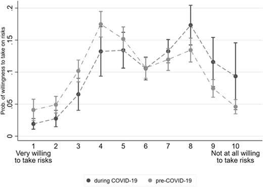
Marginal impact of COVID-19 on individual willingness to take risks.
Note: Covariates taken at mean values.
4. Discussion
In this study, we analyse whether HORAs change with the onset of COVID-19, as measured by an incentivized risk apportionment elicitation task. Once we control for heterogeneity in socioeconomic characteristics and the theoretical relationship between HORA measures, we find an overall increase in risk averse behaviour during COVID-19. We find similar results using a self-reported hypothetical risk question. In both measures, the increase in risk aversion is slightly smaller for low-income individuals (less than $20,000 a year).
Our results are mostly in line with the findings of recent literature using other incentivized risk elicitation methods and suggesting heterogeneous changes in risk attitudes. While there is no consensus on which incentivized risk measure is the most accurate to measure risk averse behaviour (Charness et al., 2013; Holzmeister and Stefan, 2021), an increase in risk averse behaviour during the COVID-19 outbreak is found across various samples using different elicitation methods. Our work provides further evidence on this using a model-free elicitation task.
COVID-19 affected everyone as the economic downturn is generalized, impacting individuals across socio-economic characteristics. Moreover, the pandemic did not discriminate across economic activities, with 20 out of 22 industry groups declining on average 31.4% in the second quarter of 2020 (Bureau of Economic Analysis, 2020). Consistent with our results, Mussio and de Oliveira (2021) find that for a sub-sample of our pre-COVID participants, the response to an increase in (financial) background risk depends on their income level. In this study, lower income participants also increase the number of risk averse choices taken but less than higher income participants. Almost 70% of our sample stated that they received financial assistance from the US government before May 2020, which could have partially relieved the impact of the pandemic on income volatility. In addition, prior literature shows that low-income workers reduced their spending less in comparison to high-income workers due to increased government assistance, which could be one of the reasons behind our risk aversion results.
A second finding in our paper is that there are no changes in either prudence or temperance under the risk apportionment methodology. Our null prudent and temperate results could be driven by their subjective expectations of the future and financial assistance received by our participants. Almost 70% of our sample reports some form of financial support from the government, regardless of whether we define them as low or high income. Consistent with prior literature on the impact of background risk on financial behaviours, federal and state financial support could be acting as additional and secure precautionary savings, which is the prudent and temperate behaviour usually observed when individuals try to offset increases in background risk (Elmendorf and Kimball, 2000; Edwards, 2008). Although COVID-19 was followed by a clear economic slowdown, our participants do not have negative future income expectations in response to the pandemic. A large percentage (87.5%) of our participants states that their financial situation might remain unchanged or improve in the next year. An overwhelming number of our participants also state that they are getting along or are comfortable/prosperous in terms of their current financial situation (93%).
To deal with a large-scale health crisis like COVID-19, policy-makers are deploying a wide-range of tools from public health messaging to lockdown measures. Risk attitudes will play an important role in how individuals will respond to these policies. Therefore, it is crucial to learn about the risk attitudes of the population and our study is a step in that direction. Future research should follow-up on our findings to examine whether the COVID-19 had a temporary or long-term effect on HORAs. Another valuable avenue to explore is to study how risk attitudes as measured by experimental tasks predict ‘real-world’ risky decision-making during the pandemic, such as mask use, mobility, and vaccination decisions.
Supplementary material
Supplementary material is available on the OUP website. These are the data, replication files, and the Online Appendix, which contains the experimental instructions and post-experimental questionnaires.
Funding
This work was supported by the McMaster Institute of Research on Aging fellows fund and the Department of Resource Economics at University of Massachusetts Amherst Faculty Research Fund.
Footnotes
For an example of each type of event, see Cassar et al. (2017), Guiso (2012), and Jakiela and Ozier (2016), respectively.
Other format alternatives to measure higher order risk attitudes include multiple nested lotteries (Deck and Schlesinger, 2014, 2018; Haering et al., 2020), multiple die rolls, (Nousair et al., 2014), or eliciting individual’s compensations using a multiple price list format (Ebert and Wiesen, 2011, 2014; Heinrich and Mayrhofer, 2018).
Some of these questions were adapted from Fetzer et al. (2020).
Our socio-demographic variables do not correspond exactly to the control variables used in the regressions. For regression purposes and ease of interpretation of the results, we consider income, education, and health as binary choices, while for the matching implementation we use their original definition from our questionnaire to match as individuals as close as possible with each other.
In addition, as nearest neighbour matching might have the risk of far away neighbours or ‘bad matches’ (Caliendo and Kopeinig, 2008), we also present a kernel matching method in the Online Appendix (Table C.2). Our results with nearest neighbour and kernel matching do not differ and match the same number of participants.
We follow recommendations on socioeconomic variables from Berkowitz and Qiu (2006), Cardak and Wilkins (2009), Noussair et al. (2014), Béland et al. (2020), Li et al. (2020), and Yue et al. (2020). We also included beliefs about their financial situation in prior specifications, but we did not find significant effects of these variables.
The original Dohmen et al. (2011) survey question scale goes from 0 to 10. On account of a coding error in the first wave of data collection, the scale appeared as 1–10 to the subjects. To be consistent in our comparisons for our post-COVID data collection, we retained the 1–10 response scale.
Acknowledgements
We would like to thank two anonymous reviewers and the editor for their helpful feedback. We are grateful to Eva Mörk and Prithvijit Mukherjee for their insightful comments. We would also like to thank the participants at the e3c workshop at Loyola Behavioral Lab, the ESA around-the-clock conference 2020, and the 12th meeting of the Society for Experimental Finance for their valuable comments.
Ethics approval
This study was approved by the McMaster University Research Ethics Board, #7204.
