Economic geography aspects of the Panama Canal

Commercial traffic through the Panama Canal

Fiscal year	Number of vessels	Tons of cargo (millions)
1915	1,075	4.9
1916	758	3.1
1917	1,803	7.1
1918	2,069	7.5
1919	2,024	6.9
1920	2,478	9.4
1921	2,892	11.6
1922	2,736	10.9
1923	3,967	19.6
1924	5,230	27.0
1925	4,673	24.0
1926	5,197	26.0
1927	5,475	27.7
1928	6,456	29.6
1929	6,413	30.7

Fiscal year	Number of vessels	Tons of cargo (millions)
1915	1,075	4.9
1916	758	3.1
1917	1,803	7.1
1918	2,069	7.5
1919	2,024	6.9
1920	2,478	9.4
1921	2,892	11.6
1922	2,736	10.9
1923	3,967	19.6
1924	5,230	27.0
1925	4,673	24.0
1926	5,197	26.0
1927	5,475	27.7
1928	6,456	29.6
1929	6,413	30.7

Note: The fiscal year ends on June 30 of the respective calendar year.

Source: Department of Commerce (1930, p. 442).

Table 1

Commercial traffic through the Panama Canal

Fiscal year	Number of vessels	Tons of cargo (millions)
1915	1,075	4.9
1916	758	3.1
1917	1,803	7.1
1918	2,069	7.5
1919	2,024	6.9
1920	2,478	9.4
1921	2,892	11.6
1922	2,736	10.9
1923	3,967	19.6
1924	5,230	27.0
1925	4,673	24.0
1926	5,197	26.0
1927	5,475	27.7
1928	6,456	29.6
1929	6,413	30.7

Fiscal year	Number of vessels	Tons of cargo (millions)
1915	1,075	4.9
1916	758	3.1
1917	1,803	7.1
1918	2,069	7.5
1919	2,024	6.9
1920	2,478	9.4
1921	2,892	11.6
1922	2,736	10.9
1923	3,967	19.6
1924	5,230	27.0
1925	4,673	24.0
1926	5,197	26.0
1927	5,475	27.7
1928	6,456	29.6
1929	6,413	30.7

Note: The fiscal year ends on June 30 of the respective calendar year.

Source: Department of Commerce (1930, p. 442).

In this paper, we compare a world with the canal to one without the canal. When do we expect to see a difference between the two? There could have been some small effect of distance to the Panama Canal on trade from the time of the railway in 1850. The years of construction of the Canal from 1904 to 1914 drew some resources and people from the USA to Panama and may account for some small effect. Similarly, there might be anticipatory effects due to the canal’s imminent opening. The canal was then opened partially in 1914, but the full opening did not take place until 1920. We would thus expect 1920 to mark the greatest change to transport costs we observe and we expect to see big effects after this year. The canal continues to become more important throughout the 20th century as international trade increases, as shipping technology improves, shipping volumes increase, and as the destination markets grow, first Europe after the wars, followed by the rise of Asian countries. For these reasons, we expect a continued effect after 1914 and 1920. The effects we report for 1940 are less influenced by these other factors and isolate the gains through the change in distances. Effects for the second half of the 20th century add additional treatments through technology and the growth of destinations and are therefore harder to interpret. For this reason, we typically focus on results up to the year 1940, but we show results for later years in the Online Appendix (Maurer and Rauch, 2022).

3. Data

Our dataset aims to construct effective distances and destination market sizes as they were before the opening of the Canal, around 1900. We do not rely on information on either destination markets or domestic transport costs in the USA after the opening, since both are potentially endogenous to the new transport cost matrix. This implies that our measurement of the market potential induced by the canal is more precise in the earlier decades of the 20th century than in the later ones. For this reason, we usually focus on the time period until 1940. However, in the Online Appendix, we also report estimates over a longer time period.

The Panama Canal facilitates commerce between US coasts, but also between US and international ports. Our measure of market potential change includes both effects. To calculate how the Canal changed international market potential, we draw on a dataset on major ports in the 19th century assembled by Pascali (2017). For every country, this dataset identifies the primary ports in 1850 and assigns them the country’s respective population and GDP data for 1900. We then calculate seaborne least-cost paths and distances from every coastal county in the USA to every major international port, using a 20× 20 km grid of the world and ArcGIS’s ‘Cost Distance’ tool. We calculate these distances under two scenarios: Once with the Panama Canal being closed or not existent and once with it being open.⁴

For every mainland US county, we then calculate the effective distance from this county’s centroid to every international port. This effective distance consists of two components: The distance from the US coast to the international port calculated before and the effective distance from the respective county to the coast. For the latter, we draw on a 1890 cost matrix provided by Donaldson and Hornbeck (2016). This matrix takes into account railroads, wagon roads, and canals with different cost parameters and therefore gives a precise picture of the effective distance between counties in that period. We restrict the paths from US counties to international ports to go through coastal counties that have a port. For this, we use the list of official ports of entry into the USA as per 1910. According to the Department of Commerce and Labor (1912), there were 109 such ports (not all of them situated on the ocean coast), which we match to our coastal counties where possible.

To add the within-US cost-distances (measured in US$) and the distances to international harbors (measured in kilometres), we first transform the domestic distance matrix from monetary units to kilometres by scaling them such that the distances expressed in kilometres match the great-circle distances for the average county pair. Total effective distance between county c and international port p^int is then calculated as the minimum distance of all possible routes via all domestic ports.

d_{c p}^{int} = min [d_{c p^{dom}} + α d_{p^{dom} p^{int}}] .

One of the crucial parameters of this exercise is to define the relative cost of shipment of 1 km inland against 1 km by sea, parametrized as α. This parameter is such that α = 1 would imply that a kilometre of trade over sea costs the same as a kilometre inland, while $α = 1 / 2$ implies that trading over sea is half the cost of trading over land. Data on freight rates between Cardiff and Port Royal in Pascali (2017) suggest that transporting one ton over a straight-line mile over the ocean cost around 0.15 cents in 1890, or a bit more than 0.09 cents per km. Ocean transport was thus much cheaper than land-based transportation modes. Donaldson and Hornbeck (2016), for example, assume a cost of 0.63 cent per ton-mile for railroad transportation within the USA and even higher values for wagon transportation. We calculate the average Donaldson–Hornbeck cost for a straight-line mile, which is roughly 1.7 cents per ton-mile in 1890. Comparing this with the ocean transportation costs from above suggests an α of around $\frac{1}{11}$ ⁠. Even this might be on the conservative end, as Maurer and Yu (2008) estimate a variable cost for a ton-mile over the ocean of only 0.035 cents in 1890 dollars, with implied αs of $\frac{1}{18}$ when using railroads as the comparison and nearly $\frac{1}{50}$ when using the average Donaldson–Hornbeck values. Given these estimates, we use a value of $α = \frac{1}{10}$ in our preferred specification as a plausible, yet conservative estimate for the cost advantage of ocean-based transportation. We show robustness to including different costs in the effective distance calculation and to using different cost parametrizations.

Under these assumptions, we then calculate the minimum effective distance of every US county to every international port, with and without the Panama Canal. Calculations of minimum effective distances can be computationally intensive, but our set of port counties is small enough that we can calculate every possible route and select the minimum from all possible ones. International market potential for county c is then defined as

{MP}_{c}^{int} = \sum_{p^{int}} {(d_{c p^{int}})}^{θ} {pop}_{p^{int}},

where

d_{c p^{int}}

is the effective distance between county c and international port p^int,

{pop}_{p^{int}}

is the population of international port p^int, which is defined as the population of the port’s country divided by the number of major ports in the country. In most countries this is inconsequential, as they only have one major international port. For those countries with more ports, it means that we spread the population evenly across all ports. Using destination country population to calculate market potential is an oversimplification, however. It ignores the fact that incomes per capita across different destination countries will be different and thus their value as trading partners. We capture this by weighting country populations by their 1900 GDP per capita relative to the USA. For example, the UK receives a weight of nearly 1.1, reflecting that its GDP per capita in 1900 was about 10% higher than the one of the USA. China, on the other hand, receives a weight of only 0.13.⁵ One drawback of weighting countries by their respective GDP per capita is that we lose several destination countries, for which we only have population data. As a robustness check, we therefore also show regressions where we simply use population without any GDP weights. Table 1 in the Online Appendix provides a list of all the foreign countries that enter our market potential calculation, along with their GDP weights.

θ is the elasticity of market potential with respect to effective distance and is the second key parameter. The unit of measurement of ${MP}_{c}^{int}$ is in terms of population per cost-distance. Irrespective of parameter θ, this variable will increase by one if one person with the same GDP per capita as in the USA is added at a cost-distance of one dollar. In line with the tradition of the market potential literature (Harris, 1954), we set parameter θ to –1.

The opening of the Panama Canal changes the effective distances in the market value calculations, so that we can calculate

[{MP}_{c}^{int} | Canal]

and

[{MP}_{c}^{int} | No Canal]

⁠. Besides international market potential, the Panama Canal also affected domestic market potential in the USA, mainly by facilitating commerce between the West and East Coasts. We capture this by calculating domestic market potential analogously to international one as

{MP}_{c}^{dom} = \sum_{c^{d}} {(d_{c^{d}})}^{θ} {pop}_{c^{d}},

where c^d are all potential destination counties in the USA and pop is their 1880 population. For domestic market potential, we do not weight county populations by their relative GDP per capita. Firstly, we are not aware of such data at the county level for the USA for our time period. More importantly, within the USA it is reasonable to assume perfect mobility of workers. While this does not guarantee income equalization, it will at least make utility levels across counties equal in equilibrium, an assumption also made by Donaldson and Hornbeck (2016). However, we report a robustness check below where we use occupational earnings scores and the occupational distribution across counties to calculate population weights as of 1880.

A county’s total market potential,

{MP}_{c}^{tot}

⁠, is then simply the sum of domestic and international market potential. Our main explanatory variable calculates how this total market potential changed due to the canal:

{MPC}_{c}^{tot} = \frac{{MP}_{c}^{tot} | Canal}{{MP}_{c}^{tot} | No Canal} .

We use the ratio, which gives us a percentage change in market potential and delivers summary statistics that are straightforward to interpret. A second advantage of using a ratio here is that it does not change with the arbitrary unit of distance measurement. Finally, when we later take the log of this variable, it automatically creates differences in log market potential due to the canal.

We then merge this with county-level data on population and employment in three broad industry categories (agriculture, services, and manufacturing) compiled by Michaels et al. (2012). These data are based on the US census and are available at 20-year intervals from 1880 to 2000. They span the whole mainland USA, excluding only North Dakota, Oklahoma, South Dakota, and Wyoming, which had not obtained statehood by 1880. To further study the evolution of population just prior to the canal, we also merge in population data for 1910 from IPUMS (Ruggles et al., 2019). In addition, we also add data on manufacturing wages and land values in 1900 and 1940 from Haines and ICPSR (2010). Land values are measured as the average value of farmland and buildings per acre, manufacturing wages as the ratio of a county’s total manufacturing wage sum and total manufacturing employment. Finally, to shed lights on the potential reallocation of populations across space, we also include data on migration. Unfortunately, the historical US census does not allow us to identify all migrants. However, based on birthplace information, we can at least identify all the people that live in a state different from the one they were born in. Drawing on the full count census records available from IPUMS (Ruggles et al., 2019) for 1900 and 1940, we therefore create the share of a county’s population that was born in a different state. This at least allows us to analyse long-distance migration. We merge the ICPSR and IPUMS data with our main dataset using standard state and county codes, which might lead to some minor measurement error in the resulting outcome variables, as the Michaels et al.’s (2012) counties are created in a consistent way over time and sometimes represent combinations of counties. In addition, we also collect basic geographic control variables such as the longitude and latitude of a county’s centroid.

Table 2 provides summary statistics for these main variables of interest, computed using our preferred parameters.⁶ As this table shows, the Panama Canal increased market potential by 2.9% for the average US county. Population numbers for the average county reflect population growth of the USA over this period.

Table 2

Summary statistics for the county dataset

		Mean	Standard deviation	N
${MP}^{tot} \| No Canal$	MP, no canal	254,882	57,824	2,425
${MP}^{tot} \| Canal$	MP, canal	262,681	61,798	2,425
MPC^tot	Total MP change as ratio	1.029	0.027	2,425
pop₁₈₈₀	1880 population	20,598	43,188	2,425
pop₁₉₀₀	1900 population	31,073	80,524	2,425
pop₁₉₁₀	1910 population	35,341	101,171	2,425
pop₁₉₂₀	1920 population	42,093	122,008	2,425
pop₁₉₄₀	1940 population	52,672	166,068	2,425
pop₁₉₆₀	1960 population	71,932	245,521	2,425
pop₁₉₈₀	1980 population	90,641	301,078	2,425
pop₂₀₀₀	2000 population	113,039	378,513	2,425

		Mean	Standard deviation	N
${MP}^{tot} \| No Canal$	MP, no canal	254,882	57,824	2,425
${MP}^{tot} \| Canal$	MP, canal	262,681	61,798	2,425
MPC^tot	Total MP change as ratio	1.029	0.027	2,425
pop₁₈₈₀	1880 population	20,598	43,188	2,425
pop₁₉₀₀	1900 population	31,073	80,524	2,425
pop₁₉₁₀	1910 population	35,341	101,171	2,425
pop₁₉₂₀	1920 population	42,093	122,008	2,425
pop₁₉₄₀	1940 population	52,672	166,068	2,425
pop₁₉₆₀	1960 population	71,932	245,521	2,425
pop₁₉₈₀	1980 population	90,641	301,078	2,425
pop₂₀₀₀	2000 population	113,039	378,513	2,425

Note: In this table, the abbreviation MP stands for market potential and MPC indicates the ratio of market potential with the canal to market potential without.

Source: Author calculation.

Table 2

Summary statistics for the county dataset

		Mean	Standard deviation	N
${MP}^{tot} \| No Canal$	MP, no canal	254,882	57,824	2,425
${MP}^{tot} \| Canal$	MP, canal	262,681	61,798	2,425
MPC^tot	Total MP change as ratio	1.029	0.027	2,425
pop₁₈₈₀	1880 population	20,598	43,188	2,425
pop₁₉₀₀	1900 population	31,073	80,524	2,425
pop₁₉₁₀	1910 population	35,341	101,171	2,425
pop₁₉₂₀	1920 population	42,093	122,008	2,425
pop₁₉₄₀	1940 population	52,672	166,068	2,425
pop₁₉₆₀	1960 population	71,932	245,521	2,425
pop₁₉₈₀	1980 population	90,641	301,078	2,425
pop₂₀₀₀	2000 population	113,039	378,513	2,425

		Mean	Standard deviation	N
${MP}^{tot} \| No Canal$	MP, no canal	254,882	57,824	2,425
${MP}^{tot} \| Canal$	MP, canal	262,681	61,798	2,425
MPC^tot	Total MP change as ratio	1.029	0.027	2,425
pop₁₈₈₀	1880 population	20,598	43,188	2,425
pop₁₉₀₀	1900 population	31,073	80,524	2,425
pop₁₉₁₀	1910 population	35,341	101,171	2,425
pop₁₉₂₀	1920 population	42,093	122,008	2,425
pop₁₉₄₀	1940 population	52,672	166,068	2,425
pop₁₉₆₀	1960 population	71,932	245,521	2,425
pop₁₉₈₀	1980 population	90,641	301,078	2,425
pop₂₀₀₀	2000 population	113,039	378,513	2,425

Note: In this table, the abbreviation MP stands for market potential and MPC indicates the ratio of market potential with the canal to market potential without.

Source: Author calculation.

Conceptually, our main regression equation looks as follows:

\ln {pop}_{c t} = β \ln {MP}_{c t}^{tot} + α_{c} + τ_{t} + X'_{c} \cdot δ_{t} + ϵ_{c t} .

This relates (log) population of county c in year t to the log of market potential. The latter will be given by

{MP}_{c}^{tot} | Canal

for 1940 and

{MP}_{c}^{tot} | No Canal

for the years up to 1920. The identifying variation in market potential thus comes only from the change in market potential due to the canal. To see this more directly, define

Δ {lnMP}_{c}^{tot} = \ln (\frac{{MP}_{c}^{tot} | Canal}{{MP}_{c}^{tot} | No Canal})

⁠, let Post Opening be a dummy that is 1 for 1940 and rewrite the regression as

\ln {pop}_{c t} = β Δ {lnMP}_{c}^{tot} \cdot {Post Opening}_{t} + α_{c} + τ_{t} + X'_{c} \cdot δ_{t} + ϵ_{c t} .

Given the log–log specification, β can be directly interpreted as the elasticity of population with respect to market potential. The specification controls for county- and year-fixed effects, and we also include time-varying effects of further control variables. Our basic set of controls consists of longitude, latitude, the county’s log population in 1880, and an indicator for being a coastal dummy. We control for longitude and latitude to capture broad geographic trends. Population in 1880 is introduced as a control variable, as it might have an effect on subsequent growth, for example, due to agglomeration effects or mean reversion. Similarly, the coastal dummy is introduced in order to abstract from a general population movement to the coast. In practice, we often focus on only two time periods and run this specification as a first-difference specification between 1940 and 1900:

Δ^{1940 - 1900} \ln {pop}_{c} = β_{1} Δ {lnMP}_{c}^{tot} + X'_{c} \cdot δ + ϵ_{c} .

This has the advantage of omitting the potentially ambiguous years 1910 and 1920 and only comparing a clear pre-canal year with a clear post-canal year. Throughout the analysis, we cluster standard errors at the level of a grid of five by five degrees following Bester et al. (2011) to account for spatial correlation in all our regressions. Figure 1 shows the market potential gain due to the Panama Canal. The map interpolates information from county centroids and darker pixels show areas that benefit more. We condition in this maps on the same set of control variables we use in the regression, such as controls for latitude and longitude, coastal counties, and initial population. In the robustness checks and the Online Appendix, we also report results for specifications where we include state × year effects, time-varying effects of initial market potential levels or of distance to the coast, and other geographic controls. Figure 2 shows the other main variable in this paper, population growth from 1900 to 1940. The scale is in terms of 30 bins of equal size. Darker areas in this figure experienced more population growth.

Fig. 1

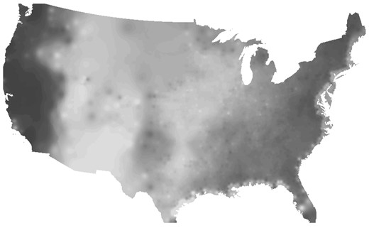
Market potential change impact of the Panama Canal, conditional on linear latitude, longitude, 1880 log population, and an indicator for coastal counties. Interpolation from county centroids. The scale is 30 equally spaced shades of gray. Darker pixels indicate areas that benefit more from the Panama Canal.

Source: Author calculation.

Fig. 2

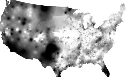
Population growth between 1900 and 1940. Interpolation from county centroids. The scale is in terms of 30 equally spaced shades of gray. Darker pixels indicate areas that experienced more population growth.

Source: Author calculation.

Market potential expressed in units of distance weighted population is a proxy for actual trade flows, which we do not observe directly. Yet, it is a useful proxy: Policy makers that evaluate the consequences of new infrastructure programs such as new railway lines or highways typically can more easily measure the implied market potential changes in units similar to ours than the implied actual trade flow changes. In our discussion of welfare effects below, we show how policy makers can translate the effect into welfare estimations.

4. Results

We start by showing a scatterplot of population growth between 1940 and 1900 and the log market potential change due to the opening of the Panama Canal in Fig. 3. As discussed above, construction of the canal started in 1904, a first opening took place in 1914, and the full opening in 1920. We therefore use 1900 as a clear pre-canal year. 1940 is an end year that gives the canal two decades since its full opening to establish its main effect. As can be seen, there is a strong positive correlation. This is also confirmed by the fitted bivariate regression line, whose parameter estimates are shown in Column 1 of Table 3. The regression coefficient is positive and strongly statistically significant, indicating that counties with improved market potential due to the Panama Canal indeed experience higher population growth. Increasing total market potential by 1% would increase the population in 1940 by 4.1% In Column 2, we additionally control for longitude, latitude, log population in 1880, and an indicator for being a coastal county, which decreases the estimate slightly. In Column 3, we move to our preferred specification, based on the full 60-year panel. We estimate a statistically significant coefficient of around 2.3, implying a long-run elasticity of population with respect to market potential above one.

Fig. 3

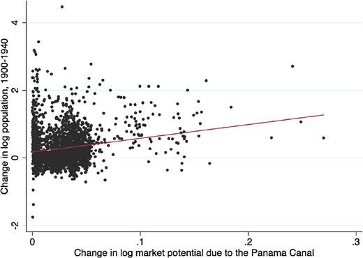
Bivariate correlation between population growth between 1940 and 1900 and the market potential change induced by the opening of the canal.

Source: Author calculation.

Table 3

The main explanatory variable is log market potential change due to the Panama Canal, in Column 3 interacted with a dummy for the year 1940

	(1)	(2)	(3)	(4)
	Δ lnpop 1940–1900		Lnpop
$Δ \ln {MP}^{tot}$	4.070^***	3.631^***	2.303^**
	(1.313)	(1.175)	(1.058)
$Δ \ln {MP}^{tot} \cdot D 1880$				0.496
				(1.932)
$Δ \ln {MP}^{tot} \cdot D 1900$				−1.438^*
				(0.829)
$Δ \ln {MP}^{tot} \cdot D 1910$				0.503
				(0.612)
$Δ \ln {MP}^{tot} \cdot D 1940$				2.193^***
				(0.568)
Observations	2,425	2,425	12,125	12,125
Specification	Long difference	Long difference	Panel 1880–1940	Panel 1880–1940
Controls	No	Yes	Yes	Yes
Clusters	47	47	47	47

	(1)	(2)	(3)	(4)
	Δ lnpop 1940–1900		Lnpop
$Δ \ln {MP}^{tot}$	4.070^***	3.631^***	2.303^**
	(1.313)	(1.175)	(1.058)
$Δ \ln {MP}^{tot} \cdot D 1880$				0.496
				(1.932)
$Δ \ln {MP}^{tot} \cdot D 1900$				−1.438^*
				(0.829)
$Δ \ln {MP}^{tot} \cdot D 1910$				0.503
				(0.612)
$Δ \ln {MP}^{tot} \cdot D 1940$				2.193^***
				(0.568)
Observations	2,425	2,425	12,125	12,125
Specification	Long difference	Long difference	Panel 1880–1940	Panel 1880–1940
Controls	No	Yes	Yes	Yes
Clusters	47	47	47	47

Notes: In Column 4, the omitted reference year is 1920. Control variables are longitude, latitude, log population in 1880, and an indicator for coastal counties. Panel regressions include year- and county-fixed effects and interact the control variables with year dummies. Robust standard errors are clustered using a chessboard grid of 5 × 5 degrees.

***

p < 0.01,

p < 0.05,

p < 0.1.

Source: Author calculation.

Table 3

The main explanatory variable is log market potential change due to the Panama Canal, in Column 3 interacted with a dummy for the year 1940

	(1)	(2)	(3)	(4)
	Δ lnpop 1940–1900		Lnpop
$Δ \ln {MP}^{tot}$	4.070^***	3.631^***	2.303^**
	(1.313)	(1.175)	(1.058)
$Δ \ln {MP}^{tot} \cdot D 1880$				0.496
				(1.932)
$Δ \ln {MP}^{tot} \cdot D 1900$				−1.438^*
				(0.829)
$Δ \ln {MP}^{tot} \cdot D 1910$				0.503
				(0.612)
$Δ \ln {MP}^{tot} \cdot D 1940$				2.193^***
				(0.568)
Observations	2,425	2,425	12,125	12,125
Specification	Long difference	Long difference	Panel 1880–1940	Panel 1880–1940
Controls	No	Yes	Yes	Yes
Clusters	47	47	47	47

	(1)	(2)	(3)	(4)
	Δ lnpop 1940–1900		Lnpop
$Δ \ln {MP}^{tot}$	4.070^***	3.631^***	2.303^**
	(1.313)	(1.175)	(1.058)
$Δ \ln {MP}^{tot} \cdot D 1880$				0.496
				(1.932)
$Δ \ln {MP}^{tot} \cdot D 1900$				−1.438^*
				(0.829)
$Δ \ln {MP}^{tot} \cdot D 1910$				0.503
				(0.612)
$Δ \ln {MP}^{tot} \cdot D 1940$				2.193^***
				(0.568)
Observations	2,425	2,425	12,125	12,125
Specification	Long difference	Long difference	Panel 1880–1940	Panel 1880–1940
Controls	No	Yes	Yes	Yes
Clusters	47	47	47	47

***

p < 0.01,

p < 0.05,

p < 0.1.

Source: Author calculation.

Our estimate is essentially a difference-in-differences estimator with a continuous treatment, given by the change in log market potential due to the canal. Given our panel, we can estimate ‘leads’ of this treatment to analyse whether population already changed systematically with future market potential change before the Canal was opened. This is done in Column 4, where instead of one Post Opening dummy, we interact the log market potential change with dummies for 1880, 1900, 1910, and 1940, the omitted reference category being 1920. We find that the market potential change due to the canal did not have an effect on population in 1880 and if anything a slight negative effect in 1900. This is reassuring, as both periods are essentially a ‘placebo check’: The canal was not open in this period and US construction had not yet started, so we would not expect to find an effect of canal-induced market potential change on population growth over those years. The effect continues to fluctuate in the years 1910 and 1920, when the canal was being constructed, and it is only in 1940, 20 years after the canal’s definitive opening, that we find a strong and positive effect of the change. In line with a causal interpretation of our results, market potential change thus only affects population in the period that experienced the impact of the finished canal.

Several recent contributions show that the effect of market potential on subsequent city growth can vary with initial city size. For example, Baum-Snow et al. (2019) find that the benefits of highway expansion in China accrued mostly to more important cities. Jedwab and Storeygard (2020), on the other hand, find that road upgrading in Africa has benefitted smaller and remote cities more. A natural question thus is whether the effects of the Panama Canal also varied with initial county population. To analyse this, we divide the counties into deciles according to their 1880 population. We then perform difference regressions for 1900–1940 on interactions of (log) total market potential changes with these deciles, controlling for the direct population effects. The resulting coefficients by initial decile are shown in Fig. 4. We do not find much evidence for heterogeneity along this dimension. Coefficients do not appear very different along the initial population distribution, the one exception being a somewhat lower effect for the initially most populated counties.

Fig. 4

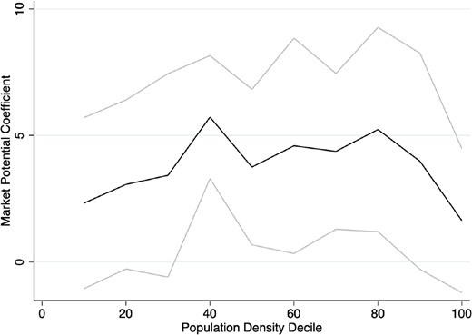
Effect by initial population. The graph shows regression coefficients of 10 indicator variables for 10 initial population deciles interacted with the main treatment effect. The gray lines show 95% confidence intervals.

Source: Author calculation.

A related concern is that the effect may be non-linear in treatment intensity. To analyse this, we run another non-parametric specification, in which we replace the total market potential change variable by 10 decile indicator variables for the intensity of treatment. Coefficients and 95% confidence intervals of this exercise are displayed in Fig. 5. The figure suggests that the treatment effect increases relatively monotonously in treatment intensity, though there is a jump around median values of market access change.

Fig. 5

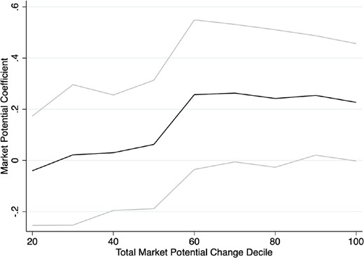
Effect by market potential change. The graph shows regression coefficient of nine indicator variables for nine treatment intensity deciles and the omitted reference category being the lowest decile of market potential change. The gray lines show 95% confidence intervals.

Source: Author calculation.

In Table 4, we analyse how the opening of the Panama Canal affected the sectoral composition of local economies. For this, we use data from Michaels et al. (2012) on employment in three broad economic sectors: agriculture, manufacturing, and services. We focus on the 1900–1940 ‘long difference’ specification akin to Column 2 of Table 3. The only change is that we additionally add control variables for manufacturing and services sectoral shares in 1880, since initial industry shares are likely to influence sectoral developments. Columns 1 and 2 show that both manufacturing and service sector employment reacted strongly to the opening of the canal. Agricultural employment, on the other hand, does not seem to be affected at all.

Table 4

Long-difference results for different sectors

	1940–1900 log difference in employment in
	Manufacturing	Services	Agriculture
$Δ \ln {MP}^{tot}$	8.199***	4.621***	−0.798
	(2.088)	(1.352)	(0.997)
Observations	2,383	2,417	2,423
Clusters	47	47	47

	1940–1900 log difference in employment in
	Manufacturing	Services	Agriculture
$Δ \ln {MP}^{tot}$	8.199***	4.621***	−0.798
	(2.088)	(1.352)	(0.997)
Observations	2,383	2,417	2,423
Clusters	47	47	47

Notes: All regressions control for longitude, latitude, log 1880 population, an indicator for coastal counties, and employment shares in manufacturing and services in the 1880. Standard errors, clustered on a 5×5 degree grid, in parentheses. ***p < 0.01, **p < 0.05, *p < 0.1.

Source: Author calculation.

Table 4

Long-difference results for different sectors

	1940–1900 log difference in employment in
	Manufacturing	Services	Agriculture
$Δ \ln {MP}^{tot}$	8.199***	4.621***	−0.798
	(2.088)	(1.352)	(0.997)
Observations	2,383	2,417	2,423
Clusters	47	47	47

	1940–1900 log difference in employment in
	Manufacturing	Services	Agriculture
$Δ \ln {MP}^{tot}$	8.199***	4.621***	−0.798
	(2.088)	(1.352)	(0.997)
Observations	2,383	2,417	2,423
Clusters	47	47	47

Source: Author calculation.

A simplification that may have some justification in the earlier parts of the 20th century would be to call manufacturing industries the tradable sector and the service sector the non-tradable sector. This simplification is less justified in later years, when services become increasingly traded. But why would non-tradable jobs react to changes in market potential? One explanation might be that tradable workers cause local demand, which in turn attracts workers in the non-tradable sector. Estimates suggest that one additional tradable job creates 0.8 (Van Dijk, 2015), 1.5 (Moretti, 2010), or 1.6 (Van Dijk, 2017) non-tradable jobs. Given these estimates, we would expect non-tradable employment to react in a way that is similar than employment in the tradable sector. The finding that the tradable and non-tradable sector reacts to market potential changes in a somewhat similar way may be of interest to theories of spatial economies. Frequently such models nest separate CES indices for tradable and non-tradable sectors in a utility function using a Cobb–Douglas function as aggregator. This would imply constant expenditures for each sector and might for many sets of assumptions on production lead indeed to similar reactions for both sectors due to market potential changes. Our results could give some empirical validation to such a modelling choice.

We consider other outcome variables in Table 5. Regressions here are based on a 1940–1900 long difference specification, except that we use different dependent variables here. In Column 1, we use the log difference in manufacturing wages, as calculated from data in Haines and ICPSR (2010). The relationship is positive and significant. We caution against overstating this result, since the wage measure suffers from a few shortcomings. It represents average manufacturing wages, without adjusting for occupation, education, age, or any other control variable. It also shows nominal wage growth, without taking into account real wage growth that could vary due to changes in house prices. In Column 2, we look at growth in agricultural land values and find a positive and significant relationship, consistent with results by Donaldson and Hornbeck (2016). Column 3 uses the change in the share of population born outside of the state on the left-hand side. Again, the relationship is positive and significant, which suggests that immigration from outside the state contributes to the population growth we find.

Table 5

The left-hand side variable uses log changes in manufacturing wages (Column 1), land values (Column 2), and the difference in the share of population born outside of the state (Column 3)

	Manuf. wage growth	Land value growth	Immigrant growth
	(1)	(2)	(3)
	1900–1940	1900–1940	1900–1940
$Δ \ln {MP}^{tot}$	1.962^***	5.120^***	3.972^***
	(0.483)	(1.294)	(0.498)
Clusters	47	47	47
Observations	1,928	2,397	2,423

	Manuf. wage growth	Land value growth	Immigrant growth
	(1)	(2)	(3)
	1900–1940	1900–1940	1900–1940
$Δ \ln {MP}^{tot}$	1.962^***	5.120^***	3.972^***
	(0.483)	(1.294)	(0.498)
Clusters	47	47	47
Observations	1,928	2,397	2,423

Notes: The right-hand side variables show the log change of total market potential due to the Panama Canal. Regressions control for longitude, latitude, log population in 1880, and an indicator for coastal counties. Robust standard errors are clustered using a 5 × 5 degree chessboard grid.

***

p < 0.01,

p < 0.05,

p < 0.1.

Source: Author calculation.

Table 5

The left-hand side variable uses log changes in manufacturing wages (Column 1), land values (Column 2), and the difference in the share of population born outside of the state (Column 3)

	Manuf. wage growth	Land value growth	Immigrant growth
	(1)	(2)	(3)
	1900–1940	1900–1940	1900–1940
$Δ \ln {MP}^{tot}$	1.962^***	5.120^***	3.972^***
	(0.483)	(1.294)	(0.498)
Clusters	47	47	47
Observations	1,928	2,397	2,423

	Manuf. wage growth	Land value growth	Immigrant growth
	(1)	(2)	(3)
	1900–1940	1900–1940	1900–1940
$Δ \ln {MP}^{tot}$	1.962^***	5.120^***	3.972^***
	(0.483)	(1.294)	(0.498)
Clusters	47	47	47
Observations	1,928	2,397	2,423

***

p < 0.01,

p < 0.05,

p < 0.1.

Source: Author calculation.

5. Robustness checks

The computation of the market potential variables in this paper relies on several assumptions. In Table 6, we assess the robustness of our key population result by varying a few of these assumptions. We always focus on the panel specification for 1880–1940. For ease of comparison, Panel A repeats our baseline result.

Table 6

Robustness checks

	(1)
	ln(pop)
	Panel A: Baseline specification
$Δ \ln {MP}^{tot} \cdot D 1940$	2.303^**
	(1.058)
	Panel B: Do not weight international populations
$Δ \ln {MP}^{tot} \cdot D 1940$	2.687^***
	(0.926)
	Panel C: Weight domestic populations
$Δ \ln {MP}^{tot} \cdot D 1940$	2.258^**
	(1.080)
	Panel D: State FE
$Δ \ln {MP}^{tot} \cdot D 1940$	−0.342
	(1.403)
	Panel E: State trends
$Δ \ln {MP}^{tot} \cdot D 1940$	2.256^**
	(1.077)
	Panel F: Additional costs
$Δ \ln {MP}^{tot} \cdot D 1940$	3.126^**
	(1.354)
	Panel G: Additional costs, Maurer and Yu (2008) parameter values
$Δ \ln {MP}^{tot} \cdot D 1940$	3.261^*
	(1.854)
	Panel H: Geometric domestic distance matrix
$Δ \ln {MP}^{tot} \cdot D 1940$	1.312^**
	(0.599)

	(1)
	ln(pop)
	Panel A: Baseline specification
$Δ \ln {MP}^{tot} \cdot D 1940$	2.303^**
	(1.058)
	Panel B: Do not weight international populations
$Δ \ln {MP}^{tot} \cdot D 1940$	2.687^***
	(0.926)
	Panel C: Weight domestic populations
$Δ \ln {MP}^{tot} \cdot D 1940$	2.258^**
	(1.080)
	Panel D: State FE
$Δ \ln {MP}^{tot} \cdot D 1940$	−0.342
	(1.403)
	Panel E: State trends
$Δ \ln {MP}^{tot} \cdot D 1940$	2.256^**
	(1.077)
	Panel F: Additional costs
$Δ \ln {MP}^{tot} \cdot D 1940$	3.126^**
	(1.354)
	Panel G: Additional costs, Maurer and Yu (2008) parameter values
$Δ \ln {MP}^{tot} \cdot D 1940$	3.261^*
	(1.854)
	Panel H: Geometric domestic distance matrix
$Δ \ln {MP}^{tot} \cdot D 1940$	1.312^**
	(0.599)

Notes: Each regression uses the 1880–1940 panel with 12,125 observations (12,120 in panel D) and 47 clusters. All regressions control for period and county-fixed effects and time-varying effects of longitude, latitude, log population in 1880, and an indicator for coastal counties. Standard errors, clustered on a 5×5 degree grid, in parentheses.

***

p < 0.01,

p < 0.05,

p < 0.1.

Source: Author calculation.

Table 6

Robustness checks

	(1)
	ln(pop)
	Panel A: Baseline specification
$Δ \ln {MP}^{tot} \cdot D 1940$	2.303^**
	(1.058)
	Panel B: Do not weight international populations
$Δ \ln {MP}^{tot} \cdot D 1940$	2.687^***
	(0.926)
	Panel C: Weight domestic populations
$Δ \ln {MP}^{tot} \cdot D 1940$	2.258^**
	(1.080)
	Panel D: State FE
$Δ \ln {MP}^{tot} \cdot D 1940$	−0.342
	(1.403)
	Panel E: State trends
$Δ \ln {MP}^{tot} \cdot D 1940$	2.256^**
	(1.077)
	Panel F: Additional costs
$Δ \ln {MP}^{tot} \cdot D 1940$	3.126^**
	(1.354)
	Panel G: Additional costs, Maurer and Yu (2008) parameter values
$Δ \ln {MP}^{tot} \cdot D 1940$	3.261^*
	(1.854)
	Panel H: Geometric domestic distance matrix
$Δ \ln {MP}^{tot} \cdot D 1940$	1.312^**
	(0.599)

	(1)
	ln(pop)
	Panel A: Baseline specification
$Δ \ln {MP}^{tot} \cdot D 1940$	2.303^**
	(1.058)
	Panel B: Do not weight international populations
$Δ \ln {MP}^{tot} \cdot D 1940$	2.687^***
	(0.926)
	Panel C: Weight domestic populations
$Δ \ln {MP}^{tot} \cdot D 1940$	2.258^**
	(1.080)
	Panel D: State FE
$Δ \ln {MP}^{tot} \cdot D 1940$	−0.342
	(1.403)
	Panel E: State trends
$Δ \ln {MP}^{tot} \cdot D 1940$	2.256^**
	(1.077)
	Panel F: Additional costs
$Δ \ln {MP}^{tot} \cdot D 1940$	3.126^**
	(1.354)
	Panel G: Additional costs, Maurer and Yu (2008) parameter values
$Δ \ln {MP}^{tot} \cdot D 1940$	3.261^*
	(1.854)
	Panel H: Geometric domestic distance matrix
$Δ \ln {MP}^{tot} \cdot D 1940$	1.312^**
	(0.599)

***

p < 0.01,

p < 0.05,

p < 0.1.

Source: Author calculation.

In our main calculation of market potential, we weighted international populations by their GDP per capita relative to the USA. The rationale behind this was that mobility across the USA would lead to a spatial equilibrium of equal utility levels, but that this could not be assumed for the whole world. One shortcoming of this was, however, that we lose some international destination countries for which we only have population, but not GDP per capita data. In Panels B and C, we probe the sensitivity of our results to this assumption. In Panel B, we do not use GDP weights for international population, treating population the same across the world as within the USA. The coefficient does not change much in either magnitude or statistical significance. In Panel C instead, we also weight domestic populations by their economic strength. Unfortunately, data on GDP or wages of the whole population are not available from the US census for 1880. Instead, we construct weights by drawing on the earnings score variable available from IPUMS. This variable assigns every occupation its %ile rank in the 1950 earnings distribution. It thus tells us whether counties on average have occupations that pay well or badly. We then weight counties by their average occupational earnings score relative to the national average. While this is doubtless a crude measure, it will capture differences in occupational quality across space, for example, due to the industrial structure. Panel C shows that if we use these domestic weights in addition to the GDP weights for international destinations, the estimates are again virtually unchanged.

In Panel D, we additionally introduce state- × year-fixed effects. This is a very demanding specification, as the change in market potential due to the canal of course has a strong geographical component and varies much more across states than within.⁷ As a result, our results become highly insignificant. We interpret this observation to suggest that variation within state is too subtle to be picked up by this specification. This is also borne out by Panel E, which introduces state-specific linear trends rather than fixed effects, and shows point estimates that are very similar to the baseline. Given that state- × year-fixed effects appear to be a too demanding specification to control for potential geographic confounders, we assess robustness to other such confounders in the Online Appendix.

In Panel F, we add additional costs to the market potential calculation. We impose an additional fixed costs for loading goods from domestic modes of transport to ocean ships. Following Fogel (1964) and Donaldson and Hornbeck (2016), we set this fixed cost for transshipment from one mode of transport to another at 50 cent per ton, corresponding to roughly 57 additional kilometres. Secondly, we add a toll cost to all routes via the Panama Canal. According to Huebner (1915), initial canal tolls were such that a ton of cargo cost around 90 cents, corresponding to 80 cents in 1890 dollars. We therefore add a fixed cost of 80 cents (92 km). A final complication is tariffs. Actual tariffs during our period of analysis depended on the country of origin and the type of good imported, which we both don’t observe and which might be endogenous to trade distances. They also were typically assessed on an ad valorem basis, making it difficult to assign a precise value per average traded ton. In our robustness check, we assign a fixed cost of 5$ (573 km). While this is a simplified approach, it captures the basic idea that tariffs made international trade more costly than domestic one. Judging from examples listed by the Treasury Department (1913), we think this parameter is similar to the tariffs levied on the few goods that were assessed on a per-ton basis, and if anything at the upper end.⁸ Reassuringly, adding these additional costs does not change our qualitative conclusion and if anything leads to a slightly larger point estimate. In Panel G, we perform a similar exercise, but using different cost parameters that are based on the calculations of Maurer and Yu (2008), who estimate (in terms of 1890 dollars) a cost advantage of sea transport of around 50, as well as a fixed transshipment cost of $1.09 (net of toll costs). The results are very similar to Panel F, albeit a bit less precise.

Finally, in Panel H, we use the same way of calculating effective distances as before, but replace the domestic transport cost matrix from Donaldson and Hornbeck (2016) by a simpler matrix based on geometric distances. This is of course a more crude measure of distance and hence of market potential change. The estimate remains positive and statistically significant, but is lower than our baseline estimate, which is consistent with this measure being less precise.

6. Welfare and cost–benefit analyses

To assess the overall welfare impact of the Panama Canal on the US economy requires the use of a general equilibrium model. In the Online Appendix, we apply a model developed by Redding (2016) to compute welfare gains from the canal. This exercise suggests that the canal led to a 0.2% increase in welfare in the year 1940. The cost of the Panama Canal was 352 million nominal USD in 1914. Using conventional inflation indices, this roughly corresponds to 10 billion USD in 2018 USD. The cost of the canal corresponds to 0.88% of US GDP at the time, which in 1913 was around 40,000 million nominal USD (Maddison, 2007). This exercise suggests that the costs of the canal were greater than the gains realized in 1940. However, when aggregating these annual welfare gains over a few years, the benefits of the canal easily outweigh the costs. There are several caveats to this exercise, which we also discuss in the Online Appendix.

7. Conclusion

This paper presents three main contributions. First, it uses exogenous variation in market potential provided by the opening of the Panama Canal to estimate the elasticity of population with respect to market potential. This elasticity is an important parameter for policy makers that try to evaluate the potential benefits of transport infrastructure such as a new railway or highway. We find that a 1% increase in market potential increased population by around 2.3% in the medium to long run. This sizable elasticity can help explain the well-established fact (Rappaport and Sachs, 2003) that the US population is disproportionately located near the coasts. We also show similar results for the growth of manufacturing wages, agricultural land values, and immigration from out of state. Second, we show that this effect seems to be fairly similar for tradable and non-tradable industries.

Finally, we use a general equilibrium framework to provide a cost–benefit analysis for the Panama Canal, one of the largest infrastructure projects in the history of the USA. It suggests that the canal did indeed increase US welfare and that its benefits outweighed its costs.

Supplementary material

Supplementary material is available on the OUP website. These are the data, replication files, and the Online Appendix.

Funding

This work was not supported by funding outside of our universities.

Footnotes

We use distance weighted population measures as proxy for trade flows that we don’t measure directly. Distance-weighted population is typically also a variable that is observable to policy makers who consider to invest in transport infrastructure.

See, for example, Atack et al.(2010), Hornung (2015), Jedwab and Moradi (2016), Berger and Enflo (2017), Bogart et al.(2018), Donaldson (2018), Büchel and Kyburz (2019), and Braun and Franke (2019).

The historic information in this section draws mainly on Cameron (1971), McCullough (1977), and Maurer and Yu (2010).

Given the global scale of our analysis, and our interest in distances, we use a Azimuthal Equidistant Projection of the world, centred around 39.83N 98.58W, the geographic centre of the USA. The maps we use are based on Manson et al.(2018) for the USA, Bjorn Sandvik’s public domain map on world borders (available from http://thematicmapping.org/downloads/world_borders.php), and the Rivers and lake centreline dataset available from Natural Earth (https://www.naturalearthdata.com/downloads/10m-physical-vectors/10m-rivers-lake-centerlines/).

Data on relative GDP per capita come also from Pascali (2017) and are based on the Maddison Project Database (Bolt and Luiten van Zanden, 2014), an updated version of the Maddison (2004) database.

When decomposed, the change for domestic market potential is 1.006 and the change for international market potential is 1.036. In the world without the canal, weighted domestic market potential is 57,619 and international market potential 197,263. Domestic market potential is considerably lower than international one, which is consistent with the USA being still relatively lightly populated country in 1900. It also should be borne in mind that these values measure market potential and thus trading opportunities, not actual trade flows.

In line with this, when we regress log market potential change on a set of state dummies, the resulting R² is 86%, illustrating how the state-fixed effects remove most of our identifying variation.

For example, the tariff of 1913 stipulated a rate of 50 cent to $1.50 per ton for clay and earth, 2$ for hay, and 7$ for nitrate of saltpetre (Treasury Department, 1913).

Acknowledgements

We thank many colleagues and participants at multiple seminars and conferences for valuable comments and suggestions. We also thank Luigi Pascali for sharing his dataset of major ports.

References

Atack

Bateman

Haines

Margo

R.A.

(

2010

)

Did railroads induce or follow economic growth? Urbanization and population growth in the American Midwest, 1850–1860

Social Science History

171

–

Bakker

J.D.

(2019)

International trade and regional inequality, Working paper.

Bakker

J.D.

Maurer

Pischke

J.-S.

, and

Rauch

(

2021

)

Of mice and merchants: Connectedness and the location of economic activity in the iron age

The Review of Economics and Statistics

–

Banerjee

Duflo

Qian

(

2012

) On the road: Access to transportation infrastructure and economic growth in China, NBER working paper 17897.

Baum-Snow

Henderson

J.V.

Turner

M.A.

Zhang

, and

Brandt

(

2020

)

Does investment in national highways help or hurt hinterland city growth?

Journal of Urban Economics

115

103124

Berger

Enflo

(

2017

)

Locomotives of local growth: the short- and long-term impact of railroads in Sweden

Journal of Urban Economics

124

–

Bester

C.A.

Conley

T.G.

Hansen

C.B.

(

2011

)

Inference with dependent data using cluster covariance estimators

Journal of Econometrics

165

137

–

Bleakley

Lin

(

2012

)

Portage and path dependence

The Quarterly Journal of Economics

127

587

–

644

Bogart

You

Alvarez

Satchell

Shaw-Taylor

(

2018

) Were railways indispensable for urbanization? Evidence from England and Wales, Working paper.

Bolt

Luiten van Zanden

(

2014

)

The Maddison project: Collaborative research on historical national accounts

Economic History Review

627

–

Bosker

, and ,

Buringh

(

2017

)

City seeds: Geography and the origins of the european city system

Journal of Urban Economics

139

–

Braun

S.T.

Franke

(

2019

) Railways, growth, and industrialisation in a developing german economy, 1829–1910, Working paper.

Büchel

Kyburz

(

2019

)

Fast track to growth? Railway access, population growth and local displacement in 19th century Switzerland

Journal of Economic Geography

155

–

195

Cameron

(

1971

)

The Impossible Dream: The Building of the Panama Canal

Hodder and Stoughton

Campante

Yanagizawa-Drott

(

2018

)

Long-range growth: Economic development in the global network of air links

The Quarterly Journal of Economics

133

1395

–

458

Cosar

A.K.

Fajgelbaum

P.D.

(

2016

)

Internal geography, international trade, and regional specialization

American Economic Journal: Microeconomics

–

Davis

Weinstein

(

2002

)

Bones, bombs, and break points: the geography of economic activity

American Economic Review

1269

–

Department of Commerce

. (

1930

)

Statistical Abstract of the United States 1930

Government Printing Office

Washington

Department of Commerce and Labor

. (

1912

)

The Foreign Commerce and Navigation of the United States for the Year Ending June 30, 1911

Government Printing Office

Washington

Donaldson

(

2018

)

Railroads of the Raj: Estimating the impact of transportation infrastructure

American Economic Review

108

899

–

934

Donaldson

Hornbeck

(

2016

)

Railroads and American economic growth: A ‘market access’ approach

The Quarterly Journal of Economics

131

799

–

858

Ducruet

Juhasz

Nagy

D.K

Steinwender

(

2020

) All aboard: The effects of port development, NBER Working Paper No. 28148.

Duranton

Turner

M.A.

(

2012

)

Urban growth and transportation

The Review of Economic Studies

1407

–

Ellingsen

(

2020

) Free and protected: Trade and breaks in long-term persistence, Job market paper.

Feyrer

(

2009

) Distance, trade, and income—the 1967 to 1975 closing of the Suez canal as a natural experiment, NBER working paper no. 15557.

Faber

(

2014

)

Trade integration, market size, and industrialization: Evidence from China’s national trunk highway system

The Review of Economic Studies

1046

–

Fajgelbaum

Gaubert

(

2018

) Optimal spatial policies, geography and sorting, NBER working paper no. w24632.

Fajgelbaum

Redding

S.J.

(

2014

) External integration, structural transformation and economic development: Evidence from Argentina, 1870–1914, NBER working paper no. w20217.

Fogel

R.W.

(

1964

)

Railroads and American Economic Growth: Essays in Econometric History

Johns Hopkins University Press

Baltimore

Frankel

J.A

Romer

D.H.

(

1999

)

Does trade cause growth?

American Economic Review

379

–

Haines

M.R

.; Inter-university Consortium for Political and Social Research (ICPSR). (

2010

)

Historical, Demographic, Economic, and Social Data: The United States, 1790–2002

Inter-university Consortium for Political and Social Research

Ann Arbor

Hanlon

W.W.

(

2017

)

Temporary shocks and persistent effects in urban economies: Evidence from British cities after the U.S. civil war

Review of Economics and Statistics

–

Harris

C.D.

(

1954

)

The market as a factor in the localization of industry in the United States

Annals of the Association of American Geographers

315

–

Heblich

Redding

S.J.

Zylberberg

(

2020

) The consequences of trade: Evidence from the repeal of the corn laws, Working paper.

Herzog

(

2021

)

National transportation networks, market access, and regional economic growth

Journal of Urban Economics

122

103316

Hornung

(

2015

)

Railroads and growth in Prussia

Journal of the European Economic Association

699

–

736

Huebner

G.G.

(

1915

)

Economic aspects of the Panama Canal

The American Economic Review

816

–

Hugot

Umana Dajud

(

2016

) Trade costs and the Suez and Panama Canals, CEPII working paper no.

2016

–

Hutchinson

W.K.

Ungo

(

2004

) Social saving of the Panama Canal, University of Vanderbilt working paper no. 04-W23.

Jedwab

Moradi

(

2016

)

The permanent effects of transportation revolutions in poor counties: Evidence from Africa

Review of Economics and Statistics

268

–

Jedwab

Storeygard

(

2020

) The average and heterogeneous effects of transportation investments: Evidence from Sub-Saharan Africa 1960–2010, NBER working paper no. 27670.

Maddison

(

2004

)

The World Economy: Historical Statistics

OECD Development Centre

Paris

Maddison

(

2007

)

Contours of the World Economy 1-2030 AD: Essays in Macro-economic History

Oxford University Press

Manson

Schroeder

Van Riper

Ruggles

(

2018

) IPUMS National Historical Geographic Information System: Version 13.0 [Database], University of Minnesota, Minneapolis.

Maurer

Rauch

(

2022

) Economic Geography Aspects of the Panama Canal. (Online Appendix, posted on author website on 20 January 2022.)

Maurer

(

2010

)

The Big Ditch: How America Took, Built, Ran, and Ultimately Gave Away the Panama Canal

Princeton University Press

Maurer

(

2008

)

What TR took: The economic impact of the Panama Canal, 1903–1937

The Journal of Economic History

686

–

721

McCullough

D.G.

Herrmann

(

1977

)

The Path between the Seas: The Creation of the Panama Canal, 1870–1914

Simon and Schuster

New York

Michaels

Rauch

Redding

(

2012

)

Urbanization and structural transformation

The Quarterly Journal of Economics

127

535

–

Michaels

Rauch

(

2018

)

Resetting the urban network: 117-2012

The Economic Journal

128

378

–

412

Moretti

(

2010

)

Local multipliers

American Economic Review

100

373

–

Ortega

Peri

(

2014

)

Openness and income: the roles of trade and migration

Journal of International Economics

231

–

Pascali

(

2017

)

The wind of change: Maritime technology, trade and economic development

American Economic Review

107

2821

–

Potlogea

A.V.

(

2018

)

Globalization and the skilled city

Journal of Urban Economics

107

–

Rappaport

Sachs

J.D.

(

2003

)

The United States as a coastal nation

Journal of Economic Growth

–

Redding

S.J.

(

2016

)

Goods trade, factor mobility and welfare

Journal of International Economics

101

148

–

Redding

S.J.

Sturm

D.M.

(

2008

)

The costs of remoteness: Evidence from German division and reunification

American Economic Review

1766

–

Redding

Venables

A.J.

(

2004

)

Economic geography and international inequality

Journal of International Economics

–

Ruggles

Flood

Goeken

Grover

Meyer

Pacas

Sobek

(

2019

) IPUMS USA: Version 9.0 [dataset]. IPUMS, Minneapolis, MN.

Secretary of Treasury

. (

1900

)

Statistical Abstract of the United States 1900

Government Printing Office

Washington

Treasury Department

. (

1913

)

The Tariff Act of October 3, 1913 on Imports into the United States

Government Printing Office

Washington

Umana Dajud

(

2017

) Domestic transport costs, Canada, and the Panama Canal, CEPII working paper no

2017

–

van Dijk

J.J.

(

2015

)

Local multipliers in United States cities: a replication of Moretti (2010)

University of Oxford

Department of Economics

Working Papers No. 771.

van Dijk

J.J.

(

2017

)

Local employment multipliers in US cities

Journal of Economic Geography

465

–