


Abstract
We investigate the impact that two German energy reforms—phase-out of nuclear power plants after the Fukushima incident and expansion of renewables due to fixed feed-in tariffs—had on neighbouring countries’ consumers. The unilateral German reforms generated substantial negative and positive impacts, respectively, in neighbouring countries with the highest overall effect of German policy found in France, not Germany; an annual negative impact on consumers of €3.15 billion. We also find significant differences in market integration between neighbouring countries by calculating ratios between the estimated policy decisions’ impacts before and after controlling for interconnector congestion.
Our vision is of an integrated continent-wide energy system where energy flows freely across borders, based on competition and the best possible use of resources, and with effective regulation of energy markets at EU level where necessary.(European Commission, 2015, A Framework Strategy for a Resilient Energy Union with a Forward-Looking Climate Change Policy, Brussels1)
1. Introduction
Cross-border trade in electricity is growing rapidly, albeit from a low base compared with other energy sources (Oseni and Pollitt, 2014). The Western European interconnector system is a leading example, benefiting from a strong push provided by the three Energy Directives, plus Swiss cooperation. International trade of electricity in OECD Europe reached around 10% of gross production in 2011 (Baritaud and Volk, 2014, Fig. 42). As with other forms of trade, there are clear benefits in aggregate: Booz and Company et al. (2013) estimate the gross welfare benefits from cross-border trade in Europe will eventually amount to an average of €6.7/MWh. At the same time, trade in electricity leads to tensions between national energy policies and wider European effects.
In this context, our paper examines the monetary impact on its neighbours of two recent reforms in the German market, Europe’s biggest power market and one with significant imports and exports of electrical power. These are the nuclear shutdown response to the Fukushima earthquake and the contemporaneous expansion of renewables. We find that both unilateral reforms had substantial—opposing—impacts on market prices in neighbouring countries. While the nuclear phase-out triggered price increases of up to 25%, the price reductions caused by Germany’s renewable energy support schemes were up to 0.16% for each percentage point of additional generation from German renewables.
Furthermore, we construct a counterfactual that enables causal inference of the degree of market integration by capturing the impact of cross-border congestion. Germany’s neighbouring countries exhibit large differences in this respect. Our empirical findings emphasize the need for increased efforts to harmonize national energy policies—especially against the background of renewable energy and climate targets in general—with relevance beyond the European Union.
The paper is structured as follows. Section 2 briefly reviews the benefits and current extent of electricity market integration in the European Union. Section 3 then characterizes the interplay between market integration processes and unilateral policy reforms and covers the German unilateral policy decisions. Section 4 presents our empirical analysis, subdivided into the description of the data set, the development of our empirical approach as well as detailed discussion of our estimation results. Section 5 concludes the paper with a summary of the main insights and a discussion of policy conclusions.
2. The benefits of electricity market integration in the European Union
European energy policy is undergoing a lengthy (and ongoing) integration process. Initially, national electricity markets were heavily regulated, state-supported monopolies that first needed to be liberalized and harmonized before a serious integration process could commence (see generally Serralles, 2006).
A key driver is the European Union’s expectation of clearly positive welfare effects associated with development of the respective market integration processes. As Antweiler (2016) explains, although electricity is in one sense homogeneous, given differing demand patterns and generation techniques, cross-border trade should be manifest in bi-directional flows which take advantage of arbitrage opportunities. Following, for example, Domanico (2007) or Serralles (2006), this is believed to have four potential impacts.
First, it should increase competition, thereby pushing the respective providers towards cost reductions and/or productivity increases through innovation. More efficient utilization of existing generation and network capacities should lower electricity prices for customers. Second, a given security of supply level can be guaranteed with reduced spare capacities, essentially because an interconnected internal market makes it easier to balance fluctuations in demand in a particular country. Third, this balancing effect is becoming increasingly important with the increasing desire for environmental protection exhibited through expansion of intermittent wind and solar energy. Fourth, these (interrelated) beneficial effects of an internal electricity market arguably enhance the overall competitiveness of the European Union’s energy intensive industries by contributing affordable, secure and sustainable energy supply.
The benefits of electricity market integration—alongside assessments of its current degree—have been the focus of several prior studies. In a detailed survey of integration benefits, Booz & Company et al. (2013) subdivide the existing literature into studies estimating the benefits of: (1) full market integration; (2) market coupling;2 and (3) market liberalization.3 In the first category, Neuhoff et al. (2013) quantify the effect of further integration of mainland-European electricity markets and the benefits from the utilization of additional wind capacity.4 In the second, Newbery et al. (2015) estimate the potential EU benefit of coupling interconnectors to increase efficiency of trans-border trading. In the (more specific) literature aimed at identifying the degree of market integration, several studies apply pairwise price tests such as price ratios, correlations and co-integration analysis and typically find an increase in integration over time. Examples include Robinson (2007), Zachmann (2008), Mjelde and Bessler (2009), and Nitsche et al. (2010).
De Menezes and Houllier (2015) analyse whether price volatility and market integration has changed across EU electricity markets after the German nuclear phase-out through correlation and co-integration analyses. Böckers and Heimeshoff (2014) study the convergence process of European wholesale electricity markets using national bank holidays as exogenous demand shocks across their two subsamples 2004–2008 and 2008–2014. They estimate a reduced form and consider demand dynamics indirectly through calendar dummies. However, they do not identify the actual degree of integration, nor do they make comparison with a full integration counterfactual. In this paper, we apply a novel approach to estimate such counterfactual prices, which enables us to compute a measure for the degree of market integration.
3. Market integration and unilateral policy reforms
Although there is no doubt that measures increasing integration of European electricity markets are likely to create substantial societal benefits, they also increase the potential impact of unilateral policy reforms on neighbouring countries; spot prices for electricity in one country become increasingly dependent on other single Member States’ actions. These can result in negative impacts, which might raise policy discussions or even storms of protest (in the worst case damaging the idea of Europe).
Furthermore, such negative impacts are likely to go beyond short-term price increases to impacts on medium- and long-term investment decisions, even resulting in failures of national energy policies. For example, German government subsidies for renewable energies together with the improved interconnection of the German-Austrian and French markets may have a knock-on effect on, for example, the profitability of a proposed French investment in construction of a thermal power plant. Indeed, there are already discussions on mechanisms to reduce interconnection aiming at protecting national electricity markets from externalities through unilateral neighbours’ policies, i.e. ‘grid-locks’ between Germany and Poland (see Puka and Szulecki, 2014).
In this context, we analyse empirically the impacts of two distinct unilateral German policy reforms: the phase-out of nuclear power plants after the Fukushima incident in March 2011 and promotion of renewables that started in 2000 and was since reformed several times. Clearly, there are differences. First, while the nuclear phase-out was a single, sudden, unilateral decision with no comparators in other European countries, most European countries promote renewables and many have revised their policies over time.
Second, we expect opposing impacts of the two policy reforms. Whilst removing a substantial fraction of nuclear power is likely to increase spot prices (provided that cross-border capacities are available and sufficiently large), promoting renewable energy production is likely to create a downward trend on price, since renewable generation at zero marginal costs reduces the residual demand on conventional generation (the so called ‘merit-order effect’).
We investigate not only whether the two unilateral reforms caused the expected effects, but also quantify them in terms of percentage price changes in neighbouring countries arising from Germany’s unilateral policy reforms.
3.1 Nuclear phase-out in Germany
The events of Fukushima in March 2011 marked a complete switch in Germany from a 2010 policy favourable to nuclear power to a sudden decision to shut-off all the six active nuclear power plants opened before 1981. This was an event of some significance: 6.3 GW of capacity, around 7% of installed conventional capacity and 12% of average German load, was permanently removed from the system, with significant impacts on nuclear plant output, as indicated in Fig. 1.
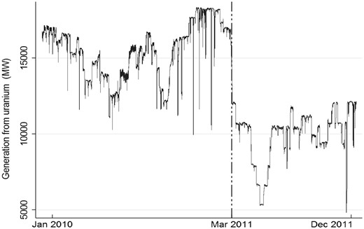
Generation from German nuclear power plants before and after the nuclear phase-out. Note: The dashed vertical reference line indicates the time of permanent closure of the 6.3 GW taken offline in March 2011 directly after the Fukushima Daiichi nuclear incident. An additional temporary drop in generation capacity from nuclear sources—to a minimum marginally above 5 GW—in May and June 2011 was caused by obligatory security checks of the remaining nuclear plants. Source: Grossi et al. (2017).
Naturally, the removal of a significant fraction of generation capacity is expected to cause price increases on the spot and future markets. In particular, nuclear capacity provides a base-load power source, consistently generating at low marginal costs to satisfy minimum demand. Removing a significant fraction of this capacity forces a switch to more expensive (lignite, hard coal or gas-fired) power plants—located nearer to the right-hand side of the supply-cost curve (merit order)—in order to meet demand (e.g. Knopf et al., 2014). The existing literature on the (price) effects of nuclear power plant closures confirms the general argument.5
3.2 Promotion of renewables in Germany and neighbouring countries
Germany had actively promoted the growth of renewable energy production long before Fukushima by implementing three basic principles: (1) investment protection through guaranteed feed-in tariffs for 20 years, with unlimited priority feed-in to the grid and connection requirements imposed on the system operator; (2) subsidies paid not by taxes but by domestic consumers as an Erneuerbare-Energien-Gesetz (EEG) surcharge included in the electricity bill;6 and (3) feed-in tariffs for new renewable plants, decreasing at regular intervals to create cost pressures (and innovation incentives) on renewable energy companies.
Although the EEG was successful in making Germany a world pioneer in renewable energy from wind and especially solar sources7 (Joskow, 2011; Borenstein, 2012), renewable capacity—as noted by Grossi et al. (2017)—is utilizable nowhere near as intensively as conventional sources, and due to its stochastic nature is not ‘biddable’ according to electricity demand in the same way as coal, gas and pumped hydro plants are (Joskow, 2011). While an average thermal plant in practice provides around 50% of its total theoretical capacity over a year, wind hovers around 20% and photovoltaic only around 11%.
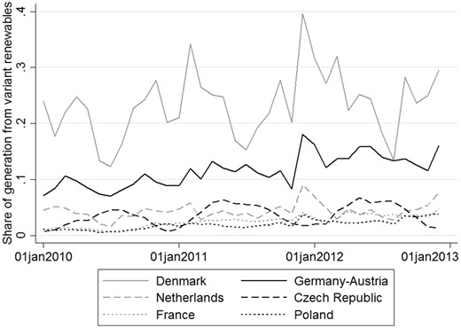
We should highlight the difference between the nuclear phase-out and the expansion of generation from renewable sources. Whilst the nuclear phase-out is a single natural experiment in that it was un-planned, the increase of renewable generation capacity is a multi-year programme benefiting owners of renewable plants with priority feed-in to the grid and fixed feed-in-tariffs for a period of 20 years, hence rendering renewable generation exogenous. Generation from renewables creates permanent supply shocks for conventional power plant owners. Importantly—by contrast with the nuclear phase-out—promotion of renewable energy production was also introduced (and incrementally extended) in Germany’s neighbouring countries.8Figure 2 plots the respective country shares of intermittent renewable energy in gross final energy consumption between 2010 and 2012. Denmark and Germany-Austria are the ‘intermittent variable renewable leaders’ with shares reaching (on average) 25% and 15%, respectively, in 2012. France, the Netherlands, the Czech Republic and Poland lag far behind, with shares around 5%. The intermittent nature of generation from wind and solar is evident in the figure (see also Grossi et al., 2017) and means that controls for these effects are necessary in isolating the impact of the German reforms on the respective spot prices.
Share of intermittent renewable energy in total electricity generation. Note: Legend is ordered from highest to lowest shares of renewable energy generation in total energy generation. Renewables include wind and solar. Switzerland excluded due to negligibly small intermittent renewables. Source: Authors’ calculations from official country data.
The impact of German unilateral energy policy reforms on market prices also allows a trade theory interpretation9 in terms of studying the welfare effects of policy measures such as tariffs/taxes or subsidies on consumers and producers in the trading partners’ countries as well as the originator. For example, a tariff or subsidy can improve the terms of trade of the (large) originating country while imposing a negative impact on social welfare on the trading partners (see, for example, Krugman et al., 2014).
Here, an application of basic trade theory would suggest that Germany—if it reduces the price of its imports by expanding renewables—could improve its welfare (with the overall net effect on welfare being dependent on the size of the ‘renewables subsidy’). Yet, assuming the loss of nuclear capacity raises the relative price of imports from neighbouring countries, a countervailing decrease in its welfare would result. For the trading partners, Germany’s renewable subsidy is expected to increase net welfare due to lower import prices whilst the nuclear reduction likely has the opposite effect.10
However, it is important to recall a distinctive feature: Germany as the originating state was not aiming at increasing short-run welfare at the expense of the trading partners through an application of standard ‘beggar-thy-neighbour’ policies known from strategic trade theory (see, for example, Brander and Spencer, 1985), but had in mind longer-run environmental goals. While different in motivation, the effects on the trading partners can be quite similar (i.e. they either profit or suffer from the unilateral German decisions). We study the existence and size of the effects on market prices empirically below.
4. Empirical analysis
How significantly are neighbouring countries affected by Germany’s unilateral policy decisions? In a highly integrated market, both actions—the sudden nuclear phase-out and the expansion of renewables through support schemes—may be expected to cause substantial knock-on effects, while if the country is not integrated at all with Germany, we would expect zero impact. By combining this with information on import and export cross-border congestion, the degree of market integration can be measured. More significantly, however, the degree of interdependence raises the question of whether the project of integrating European energy markets is in danger if unilateral decisions of certain Member States have substantial effects on medium- and long-term investment decisions in neighbouring countries as well as on short-term prices.
We provide an empirical assessment of the impacts of the two unilateral energy policy reforms in Germany on wholesale electricity prices in its directly connected neighbours: the Netherlands, France, Poland, the Czech Republic, Switzerland and Denmark (West and East). Spain is used in a placebo test since, being unconnected directly or indirectly with Germany, it would not be expected to be affected by either change.11 Section 4.1 describes the construction of the data set and presents descriptive statistics, Section 4.2 describes our modelling approach. The estimation results are in Section 4.3.
4.1 Data set and descriptive statistics
We collected and merged data from several sources over the calendar years 2010 to 2012 to create the rich, unique data set used for our empirical analysis. Our dependent variables are country-specific wholesale (spot) day-ahead prices obtained from the respective power exchanges: EPEX Spot for Germany-Austria, France and Switzerland, Elspot for the two Danish zones (West and East), PXE for the Czech Republic, PPX for Poland and APX for the Netherlands. All price series are collected on an hourly basis, but transformed into daily averages, in order to maintain analytical tractability.
Our independent variables are of two broad types. Starting with the individual variables, hourly data on observed load in each country was obtained from European network of transmission system operators for electricity (ENTSO-E), while information on hourly forecasted generation from the intermittent renewables wind and solar (for each country) comes from the commercial data provider Eurowind GmbH. To control for cross-border congestion, we have collected hourly data on the import and export interconnectors available for trade (Available Transfer Capacities [ATC]). This comes partly from the respective transmission system operators (TSOs) TransnetBW, 50 Hertz, Amprion (all three Germany), TenneT (Germany and the Netherlands), RTE (France), Energienet.dk (Denmark), CEPS (Czech Republic), PSE (Poland) and SwissGrid (Switzerland) and partly—due to changes in the responsibility for the allocation of interconnector capacity—from the Auction Offices CAO (for the Central Western Europe (CWE) area) and CASC (for the Central Eastern Europe [CEE] area). We use this to calculate daily import and export congestion indices, defined as the percentage of hours of a day over which the respective interconnectors were congested. Congestion prevents further trans-border trade that would otherwise continue until prices equalize and arbitrage possibilities vanish. As common variables, we include monthly European hard coal and natural gas price indices (base year 2005)—obtained from the Federal Statistical Office of Germany—and an EU ETS carbon emission price index (which was downloaded from Thomson Reuters Datastream).
Since load is likely endogenous, we instrument for it in our econometric analysis below. Our instruments for load are the current level of area-specific air temperatures in each country and their squares. Data on daily air temperatures in many cities in Germany and its neighbouring countries have been downloaded from Mathematica 9 (WeatherData and CityData). This data constitutes the basis for the calculation of population-weighted temperature indices.12 The descriptive statistics for the resulting data set are reported in Table 1 and subsequently discussed selectively.
Descriptive statistics
| DE-AT | FR | NL | CH | DKE | DKW | PL | CZ | ES | ||
|---|---|---|---|---|---|---|---|---|---|---|
| Dependent Variable | ||||||||||
| Price (Euro/MWh) | 46.09 | 47.81 | 48.49 | 52.27 | 47.97 | 43.59 | 45.87 | 45.58 | 44.76 | |
| (16.00) | (25.46) | (13.75) | (17.34) | (35.23) | (15.03) | (9.93) | (15.91) | (15.53) | ||
| Individual Variables | ||||||||||
| Load (GWh) | 62.31 | 56.21 | 12.51 | 5.66 | 1.55 | 2.30 | 16.49 | 7.20 | 29.20 | |
| (11.43) | (12.92) | (2.39) | (1.10) | (035) | (0.52) | (2.79) | (1.25) | (3.13) | ||
| Wind (GWh) | 4.97 | 1.10 | 0.53 | – | 0.89 | 0.89 | 0.31 | 0.03 | 4.25 | |
| (4.12) | (0.95) | (0.47) | – | (0.78) | (0.78) | (0.30) | (0.03) | (2.37) | ||
| Solar (GWh) | 2.20 | 0.27 | – | – | – | – | – | 0.23 | 0.77 | |
| (3.61) | (0.45) | – | – | – | – | – | (0.40) | (0.28) | ||
| Import ATC (GW) | 12.10 | 2.19 | 2.51 | 4.34 | 0.52 | 0.90 | 0.53 | 1.11 | – | |
| (1.03) | (0.58) | (0.38) | (0.24) | (0.16) | (0.44) | (0.29) | (0.53) | |||
| Export ATC (GW) | 6.75 | 2.61 | 2.12 | 0.69 | 0.50 | 0.81 | 0.24 | 2.21 | – | |
| (0.90) | (0.60) | (0.39) | (0.23) | (0.20) | (0.28) | (0.24) | (0.46) | |||
| Import Congestion Index (0-1) | 0.22 | 0.18 | 0.10 | 0.23 | 0.29 | 0.32 | 0.48 | 0.42 | – | |
| (0.25) | (0.38) | (0.31) | (0.42) | (0.45) | (0.47) | (0.50) | (0.49) | |||
| Export Congestion Index (0-1) | 0.31 | 0.28 | 0.30 | 0.62 | 0.23 | 0.13 | 0.43 | 0.38 | – | |
| (0.29) | (0.45) | (0.46) | (0.48) | (0.42) | (0.34) | (0.50) | (0.49) | |||
| Common Variables | ||||||||||
| Gas Price Index | 164.85 | 164.85 | 164.85 | 164.85 | 164.85 | 164.85 | 164.85 | 164.85 | 164.85 | |
| (22.85) | (22.85) | (22.85) | (22.85) | (22.85) | (22.85) | (22.85) | (22.85) | (22.85) | ||
| Coal Price Index | 174.66 | 174.66 | 174.66 | 174.66 | 174.66 | 174.66 | 174.66 | 174.66 | 174.66 | |
| (9.98) | (9.98) | (9.98) | (9.98) | (9.98) | (9.98) | (9.98) | (9.98) | (9.98) | ||
| Carbon Price Index | 8.40 | 8.40 | 8.40 | 8.40 | 8.40 | 8.40 | 8.40 | 8.40 | 8.40 | |
| (4.16) | (4.16) | (4.16) | (4.16) | (4.16) | (4.16) | (4.16) | (4.16) | (4.16) | ||
| Instrument for Load | ||||||||||
| Temperature (°C) | 9.83 | 12.71 | 10.30 | 10.30 | 8.32 | 8.59 | 8.83 | 9.41 | 17.16 | |
| (8.00) | (6.61) | (6.26) | (7.61) | (7.03) | (7.20) | (8.99) | (8.62) | (6.40) | ||
Notes: Descriptive statistics show means and standard deviations (in parentheses) of the utilized data; ‘Import’ and ‘Export’ variables always represent flow direction from the German perspective. For countries with missing values for solar and/or wind generation, the respective values were too low to be measured. For countries outside the European Currency Union, daily exchange rates from Thomson Reuters are used for the transformation. Though Spain has no interconnection with Germany we include it for the application of a placebo test. Source: Authors’ calculations.
Table 1 shows some variation in the spot prices for electricity (expressed in Euro per MWh) between Germany and its neighbouring countries. As electricity is a homogeneous good, not trivial price differences indicate imperfectly integrated markets. In fact, spot prices are found in a range from Denmark (West) with an average price of €43.59 up to Switzerland showing an average price of €52.27, i.e. about a 19.9 % higher price.13 A summary on average absolute price differences between the German-Austrian market and its neighbours is presented in Table 2, showing that the price difference is highest with Poland and lowest with the Netherlands and Czech Republic.
Average price differences between the German-Austrian market and its interconnected neighbours
| Germany-Austria and | FR | NL | CH | DKE | DKW | PL | CZ |
|---|---|---|---|---|---|---|---|
| Average price difference in Euro/MWh | 4.9 | 3.3 | 8.2 | 8.3 | 5.2 | 9.5 | 4.2 |
| Standard Deviation of price differences | 20.4 | 8.2 | 10.4 | 31.4 | 8.6 | 10.7 | 5.5 |
| Germany-Austria and | FR | NL | CH | DKE | DKW | PL | CZ |
|---|---|---|---|---|---|---|---|
| Average price difference in Euro/MWh | 4.9 | 3.3 | 8.2 | 8.3 | 5.2 | 9.5 | 4.2 |
| Standard Deviation of price differences | 20.4 | 8.2 | 10.4 | 31.4 | 8.6 | 10.7 | 5.5 |
Source: Authors’ calculations.
Information on renewables in the form of electricity production through either wind or solar is limited to countries with an appreciable share of renewables.14 In particular solar is largely confined to a subset. Germany-Austria has by far the largest amount in both categories (4.97 GWh and 2.20 GWh), but small compared to total load.
Germany has by far the largest import and export capacities available for trade (ATC) in both categories. However, surprisingly because Germany is a net exporter, interconnector capacities for export are roughly half the size of import capacities. This is mainly because interconnector capacity from Switzerland to Germany is around five times higher than in the opposite direction. The derived import and export congestion indices—defined as the proportion of hours of the day at which the respective interconnectors were congested (thereby hindering further trans-border trade)—reveal that, in terms of imports, congestion appears to be a minor issue for the Netherlands (10%) while the opposite is true for Poland (48%). For exports, the spectrum includes 13% in the case of Denmark (West) and 62% for Switzerland.15
However, our congestion index variables cannot be interpreted as direct measures for the degrees of integration. For example, price differences can occur even if interconnector capacity is not fully utilized (depending on the allocation mode of interconnector capacity). Particularly in explicit auctions—as used between Germany and Switzerland, Poland and the Czech Republic—expectation errors of electricity traders can cause such price differences (despite some interconnector capacity being available).16 Furthermore, congestion price differences can differ significantly between countries. For instance, when congested, the price difference between Germany and the Czech Republic is, on average, €5.13/MWh, while it is, on average, €15.96/MWh when the interconnector between Denmark East and Germany is congested because Danish electricity generation (and thus its price) is much more intermittent due to their high wind share of generation reflected in Fig. 2. Also, as was shown above in Table 1, while the interconnectors between Germany and the Czech Republic are congested in 42% (imports) and 38% (exports) of the time, the average absolute price difference between Czech and German-Austrian prices is only €4.2/MWh) while it is on average €4.9/MWh between France and Germany where interconnectors suffer less frequent congestion (18% import and 28% export congestions). The same is observed when price correlations are considered. For instance, French prices are less correlated with German-Austrian prices than Czech prices, despite the fact that Czech interconnectors with Germany are more frequently congested than French interconnectors with Germany.17 Thus, average of price differences and the frequency of congestions are not necessarily related.
We further assume interconnector capacities are exogenous in the short run and unaffected by the nuclear outage. Interconnector capacity expansion is a long-term matter and variation in the transfer capacity is based on technical calculations according to the ENTSO-E method, reflecting the physical realities of the grid adjusted (varying) security margin. We also assume national fuel-fired generation capacities are exogenous and unaffected in the short-term and generation from renewables is particularly exogenous due to fixed feed-in tariffs and quota obligations provided through national renewable support schemes.18 Nevertheless, we instrument for the congestion variables later due to simultaneity with prices.
4.2 Empirical approach
Our empirical approach is subdivided into two parts. First, we estimate the impact of unilateral German policy decisions—the nuclear phase-out and the recent expansion of renewables resulting from national support schemes—on prices in its (interconnected) neighbouring countries and the German-Austrian market itself. As both the nuclear phase-out and generation from renewables are exogenous, our study has a quasi-experimental character. Second, we additionally control for the (price-increasing or price-decreasing) impact of congested interconnectors through the inclusion of import and export congestion variables, respectively, to estimate the impact the nuclear phase-out and renewable generation would have had on the neighbouring markets absent cross-border congestions. The degree of market integration is then calculated as the ratio between the estimated policy decisions’ impacts before and after controlling for congestion. For instance, if we find that Germany’s nuclear phase-out has caused a 10% price increase in one country before controlling for congestion and 20% afterwards, we measure the degree of integration between these two markets as 50%.
We believe that endogeneity is not a major issue for the remaining variables since coal, gas and emission certificates are traded supra-nationally and Germany only accounts for a fraction of the trade.
The endogenous nature of the non-parametrically modelled variable
We next apply Hardle and Mammen's (1993) specification test to assess whether the nonparametric fit can be approximated by a parametric polynomial alternative. The specification test is based on squared deviations between parametric and non-parametric regressions. Critical values are obtained, simulating by wild bootstrap. The test results justify a polynomial adjustment for load of order 2 for all countries (see Appendix Table A.2 in the Supplementary material). This information on the supply curve enables us, in a second step, to correctly model the shape of the supply curve parametrically through the inclusion of squared load as a second endogenous variable and, in addition, to consider correlation between the disturbances across countries through the estimation of system-wide two-step GMM. We instrument for the square of load with
4.3 Estimation results
Table 3 presents our main estimation results. Columns (1) and (2) report the results of the semiparametric estimation by Robinson’s (1988) method—excluding or including congestions—and columns (3) and (4) report the results of the parametric estimation by two-step IV GMM (see Appendix Tables A.4–A.11 in the Supplementary material for the respective first-stage test statistics). Note that—in columns (1) and (2)—the reported coefficients stem from 16 separate regressions (which we do not report for the sake of clarity and brevity21).
Estimation results
| (1) | (2) | (3) | (4) | |||||
|---|---|---|---|---|---|---|---|---|
| Semiparametric IV | Semiparametric IV | System IV GMM | System IV GMM | |||||
| Congestion Control | NO | YES | NO | YES | ||||
| DE-AT | ||||||||
| Phase-out | 0.152*** | (0.031) | 0.123*** | (0.038) | 0.158*** | (0.032) | 0.110*** | (0.003) |
| Renewables | −0.185*** | (0.014) | −0.164*** | (0.026) | −0.206*** | (0.020) | −0.199*** | (0.001) |
| FR | ||||||||
| Phase-out | 0.125*** | (0.046) | 0.177*** | (0.042) | 0.179*** | (0.039) | 0.232*** | (0.003) |
| Renewables | −0.083*** | (0.014) | −0.136*** | (0.021) | −0.072*** | (0.014) | −0.117*** | (0.002) |
| NL | ||||||||
| Phase-out | 0.084** | (0.034) | 0.084** | (0.038) | 0.075** | (0.035) | 0.092** | (0.002) |
| Renewables | −0.061*** | (0.013) | −0.076*** | (0.014) | −0.067*** | (0.016) | −0.085*** | (0.001) |
| CH | ||||||||
| Phase-out | 0.092** | (0.035) | 0.096** | (0.036) | 0.080** | (0.035) | 0.131*** | (0.003) |
| Renewables | −0.096*** | (0.021) | −0.116*** | (0.028) | −0.088*** | (0.016) | −0.132*** | (0.001) |
| DK East | ||||||||
| Phase-out | 0.235*** | (0.052) | 0.291*** | (0.052) | 0.248*** | (0.051) | 0.276*** | (0.004) |
| Renewables | −0.101*** | (0.032) | −0.134*** | (0.024) | −0.090*** | (0.027) | −0.123*** | (0.002) |
| DK West | ||||||||
| Phase-out | 0.110** | (0.049) | 0.153** | (0.059) | 0.089** | (0.048) | 0.102*** | (0.004) |
| Renewables | −0.157*** | (0.033) | −0.174*** | (0.026) | −0.150*** | (0.021) | −0.160*** | (0.002) |
| PL | ||||||||
| Phase-out | −0.007 | (0.037) | 0.067** | (0.036) | −0.001 | (0.034) | 0.066** | (0.002) |
| Renewables | −0.013 | (0.009) | −0.068*** | (0.014) | −0.022** | (0.010) | −0.068*** | (0.001) |
| CZ | ||||||||
| Phase-out | 0.186*** | (0.040) | 0.176*** | (0.041) | 0.198*** | (0.034) | 0.180*** | (0.003) |
| Renewables | −0.161*** | (0.037) | −0.196*** | (0.048) | −0.159*** | (0.023) | −0.179*** | (0.002) |
| #Obs. | 1095 | 1095 | 1095 | 1095 | ||||
Note: The table reports the main results from 16 separate semiparametric regressions in columns (1) and (2) and two regressions using system wide IV-GMM in columns (3) and (4). Parameters of phase-out are transformed through (exp(
Source: Authors' estimates.
Comparing regression results between the Robinson estimator and two-step system IV GMM, Table 3 shows very similar results in terms of both direction and size of the coefficients across the two estimation approaches.22 We therefore concentrate our further discussion on the results from the system GMM model shown in columns (3) and (4) which, for the reasons given above, arguably generates more efficient estimates.
Comparing the estimation results excluding congestion controls, the expected positive impact of the nuclear phase-out on spot price is confirmed for all neighbouring countries except Poland, while the promotion of renewables in Germany pushed prices down. The nuclear phase-out caused large price increases in Germany-Austria itself (16%), but also in its neighbouring countries France (18%), DK East (25%) and the Czech Republic (20%). The promotion of renewables, however, led to price decreases particularly in Germany-Austria (0.21% for a 1% increase in generation from renewables), Denmark West (0.15%) and the Czech Republic (0.16%).
Turning to the results of our estimations including congestion controls, a comparison of the respective values in columns (3) and (4) shows diverging results for coefficient magnitudes while their direction and general significance remain unaffected (again excepting Poland). In particular, we find (absolute) size reductions for both unilateral decisions—nuclear phase-out and promotion of renewables—for Germany-Austria indicating that a higher degree of market integration would have reduced the impact of German reforms on the German-Austrian market itself. Most expected neighbouring countries exhibit larger (absolute) coefficients when controlling for congestions—the impact of Germany’s reforms would have been higher if the markets were fully integrated.
Although the discussion of the empirical results of the two separate stages—excluding and including congestion controls—has provided valuable insights on the price effects of the two unilateral energy policy decisions of Germany, we ultimately want to use these results to derive a measure of the degree of market integration. In Table 4 above, we present calculations of the ratio of the estimated policy decisions’ impacts before and after controlling for congestions.23
Degree of market integration
| DE-AT | FR | NL | CH | DKE | DKW | PL | CZ | |
|---|---|---|---|---|---|---|---|---|
| Phase-out Index | 70% | 77% | 82% | 61% | 90% | 87% | 0% | 100% |
| Renewable Index | 97% | 62% | 79% | 67% | 73% | 94% | 32% | 89% |
| Mean | 83% | 69% | 80% | 64% | 82% | 91% | 16% | 94% |
| DE-AT | FR | NL | CH | DKE | DKW | PL | CZ | |
|---|---|---|---|---|---|---|---|---|
| Phase-out Index | 70% | 77% | 82% | 61% | 90% | 87% | 0% | 100% |
| Renewable Index | 97% | 62% | 79% | 67% | 73% | 94% | 32% | 89% |
| Mean | 83% | 69% | 80% | 64% | 82% | 91% | 16% | 94% |
Note: Degree of market integration is the ratio of the coefficients from the GMM estimates in Table 3 (capped at 100%). In the case of Germany, the coefficient of phase-out and renewables, respectively from column (4) is divided by the respective coefficient from column (3). For all neighbouring countries, the index is computed as the ratio of (3) to (4). Mean refers to the mean value of both market integration indices. Coefficients insignificant at 10% are considered as zero. Source: Authors’ calculations.
As Table 4 shows, the degree of market integration is mostly similar regardless of whether we measure it for the nuclear phase-out or renewable generation—the cross-country correlation24 between both types of measures is around +0.81. We would expect it to be less than 100%, because the impact is felt differently across countries due to their different circumstances.
Based on the mean of both measures, the Czech market (94%) is almost fully integrated with the German-Austrian market with the Netherlands and Denmark somewhat less so. By contrast, the lowest degree of market integration is found for Poland (16%).25 The mean value of 83% for the German-Austrian market can be interpreted as the average degree of integration of all neighbouring markets with the German-Austrian market.
In order to provide confidence that the effects we uncover are indeed associated with interconnection, we employed the same estimation strategy for the Spanish electricity market as a placebo test. Spain was chosen because it is not directly connected with Germany but is similar in generation patterns. The indirect connection via France is also relatively low. Thus, we assume that the impact of the German policy reforms on the Spanish market should be negligible and finding significant effects of the German policies on the Spanish market would suggest either that the Spanish market is more strongly connected with the German-Austrian market or—which would be worse—that our estimates of the policy effects reflect coincidental developments rather than the policy effects. However, the GMM estimates show both German policy measures had insignificant impacts on Spanish electricity prices. Details are given in Appendix Table A.12 (in the Supplementary material).
We close the section by providing some ballpark figures on the monetary effects of the two German unilateral policy reforms on its neighbours. Table 5 quantifies the yearly windfall negative and positive impacts on consumers as well as the respective (country-specific) net effects of the two unilateral reforms.26
Yearly windfall impacts on consumers from unilateral German energy policies
| in € billion/year | DE | AT | FR | NL | CH | DKE | DKW | PL | CZ |
|---|---|---|---|---|---|---|---|---|---|
| Higher costs from the phase-out | 3.23 | 0.44 | 3.73 | 0.38 | 0.19 | 0.14 | 0.07 | 0.00 | 0.51 |
| Lower costs from increased German renewables | 1.60 | 0.22 | 0.58 | 0.13 | 0.08 | 0.02 | 0.05 | 0.06 | 0.16 |
| Net impact of unilateral policies on consumers as a whole | −1.63 | −0.22 | −3.15 | −0.25 | −0.11 | −0.12 | −0.02 | 0.06 | −0.35 |
Source: Authors’ calculations.
Based on the estimated coefficients from column 3 in Table 3 and mean values of the control variables we compute hypothetical counterfactual spot prices for each country. Define the (k by c) matrix
In sum, the nuclear phase-out generated extra costs of about €8.7 billion per year for consumers in Germany and its neighbours, while the promotion of renewables caused windfall savings of about €2.9 billion yearly in the analysed post-phase-out period.30
With respect to the impact of the policy reforms on electricity producers in neighbouring countries the opposite is true: the German nuclear phase-out increased electricity prices and thus producer rents in neighbouring countries whilst the increase of German renewables reduced foreign prices and thus rents for neighbouring producers. As electricity demand is rather inelastic—and deadweight losses thus rather small—these policy reforms present potentially similarly-sized windfall costs and savings between foreign consumers and producers. However, it should be noted that, beyond these eventually mostly distributional impacts, unilateral policies are also likely to have an impact on the investment risks for foreign electricity producers, if they are unexpected.
In sum, the main result of our empirical analysis is that because most central continental European countries are already highly integrated, unilateral policy reforms have significant impacts on consumers in neighbouring countries.31 By demonstrating the substantial impact unilateral policy reforms—particularly in large countries—can have on neighbouring countries in an internal market for electricity, our results raise the question of policy implications.
5. Conclusions and policy implications
Harmonization and integration of separate national energy markets to an interconnected internal European market is a top priority for the European Commission, something we do not question here. However, as energy policy largely remains subject to national sovereignty, greater integration means unilateral national policies can impact interconnected markets. We investigated the impact of two distinct national energy reforms in Germany—the phase-out of nuclear power plants after the Fukushima incident and the expansion of renewables promoted by fixed feed-in tariffs and unlimited priority feed-in—on neighbouring countries. The phase-out triggered price increases of up to 25% in neighbouring countries whilst the renewable energy support schemes caused a price decrease of up to 0.16% for each percent of additional generation from German renewables. Also, in most cases the impact of both policy reforms would have been a little higher in the absence of cross-border congestion. The range of the identified market integration spans from 16% to 94%. However, the 16% for Poland is an outlier since the second lowest value in terms of market integration is 64% (Switzerland). Hence, the goal of a single internal electricity market with all the benefits such as an increased (and cheaper) security of supply or a power smoothing and the resulting smoothing in prices is not far away.
From a policy perspective, the externalities of unilateral decision in one Member State imposed on the others demonstrates the importance of a coordinated approach of European energy policy in a largely well-integrated European electricity market. This does not necessarily suggest that all strategic decisions are made on the European level. However, it requires significant monitoring in order that their costs and implications are discussed.
Considering the cost implications in more depth, separation into economy-specific, industry-specific and market-specific perspectives appears feasible. First, from an economy-specific (macroeconomic) perspective, increasing electricity prices act like a VAT increase on the one hand and decrease available income for consumers on the other, thereby having direct impacts on real purchasing power, hence, on industry production and economic growth in both the originating and the neighbouring countries (see also, Hamilton, 1983; Mork, 1989; Kilian, 2008; Berk and Yetkiner, 2014; Cox et al., 2014).
Second, from an industry-specific perspective, intensive energy-using firms face substantial absolute increases in costs causing a competitive disadvantage with respect to foreign competitors (either less integrated—and therefore less affected by the policy reform—or located outside Europe). If the respective price increases are permanent and substantial, unilateral policy reforms in one country may cause firm closures, and even changes in industry structures, in neighbouring countries, triggering potentially substantial knock-on effects from social and labour market perspectives, for example.
Third, from a market-specific perspective, unilateral policy reforms have a direct impact on investment decisions in neighbouring countries. For example, the Net Present Value calculation of an investor considering construction of a French power plant will depend on expectations regarding neighbours’ unilateral policy reforms, creating uncertainty in addition to positive or negative price effects. Anticipated lower prices—caused by the promotion of renewables—will reduce the incentives to invest into construction of a new plant. In any case, unilateral policy reforms will therefore impact upon the future structure of the European electricity industry. Potentially, the induced insecurity with respect to expected return on investments can cause underinvestment and thereby negative externalities on supply security.
Against this background, it appears to be important to design new rules—or alternatively enforce existing rules—on what types of decisions need debate or even decision at the Community level before they are actually implemented. Although in this article, we only provide evidence on the importance of this issue for the case of (parts of) the European electricity market, the main allocative and distributive impacts of unilateral national decisions are likely to apply to other policy areas in the European Union as well—thus suggesting the development and implementation of a comprehensive general approach that reflects the strategic importance of the issue for the future development of the European Union.
Supplementary material
Supplementary material is available online at the OUP website. This comprises an online Appendix and the data replication files. The data used in the paper are bought from commercial providers and are not publicly available. Independent researchers, however, can be given access to the data required to run the do-file at ZEW, subject to the signing of a data usage contract. The usage contract allows independent researchers to access the data, but not to take the data set away from ZEW.
Funding
This work was supported in part by the Engineering and Physical Sciences Research Council of the UK under grant number EP/K002228 to MW. We benefited from the facilities of ZEW in producing the paper.
Footnotes
Communication from the European Commission to the European Parliament, the Council, the European Economic and Social Committee, the Committee of Regions and the European Investment Bank. A Framework Strategy for a Resilient Energy Union with a Forward-Looking Climate Change Policy. COM (2015) 80 final, February 2015, p. 2.
See, for example, De Jong et al. (2007) and Kristiansen (2007a, 2007b).
See, for example, Pollitt (2009a, 2009b, 2012).
Other contributions include Leuthold et al. (2005), Green (2007), and Pellini (2014).
Using a dummy variable approach, Grossi et al. (2017) investigate the impact of the phase-out on the German market itself. They find prices in Germany have increased—most significantly in hours of low demand (caused by a shift in the merit order), with only a small price increase in hours of high demand (caused by increased market power). Davis and Hausman (2016), in a related exercise with some parallels, find comparable price effects of an unexpected nuclear power plant closure in California. Using a semi-parametric regression approach to identify the marginal generation unit each time-period before and after the event, they found the closure created binding transmission constraints, causing short-run inefficiencies and potentially making it more profitable for certain plants to act non-competitively.
In 2014, the EEG surcharge was 6.24 ct/kWh. However, energy intensive industries are widely exempted from paying the surcharge.
Capacity in these areas has been growing rapidly, boosted by EEG support. According to the German Ministry for Economic Affairs and Energy (2014), in late 2011, wind capacity reached almost 30GW with photovoltaic power capacity at about 25GW (out of a total system listed capacity of 175GW). In sum, in the year 2011, more capacity had been added through renewables (wind: 1.9GW; solar: 7.5GW) than had been removed by the nuclear phase-out.
It should be noted that we control for the simultaneous generation from renewables in the neighbouring countries in all regressions and thus capture parallel developments therein.
We are grateful to an anonymous reviewer for suggesting a discussion in light of (strategic) trade theory.
Specifically, while producers in the trading partners’ countries are expected to increase profits due to less cheap nuclear plants in Germany, the respective consumers are likely to face reductions in consumer surplus due to higher market prices.
German and Austrian markets are fully integrated and therefore considered as a single market. Although Germany and Belgium are neighbouring countries, they currently are connected only through loop flows. However, according to Jauréguy-Naudin (2012), the TSOs of the two countries were considering the construction of an HVDC line with a capacity of 1000 MW. Furthermore, the existing (small) interconnector between Germany and Sweden is excluded due to data unavailability. Spain’s interconnector with France is very limited.
To avoid problems of quadratic transformation, the temperature indices are converted into degrees Fahrenheit, which always take positive values within our data. Source: Authors’ calculations.
Dickey-Fuller and Phillips-Perron tests clearly reject the null hypothesis of a unit root in the underlying price and load series; test statistics reported in Table A.2 in the online Appendix.
Unfortunately, we do not observe Scandinavian reservoir levels which would also be relevant, in particular we would expect them to have an effect on electricity prices in Denmark. Nordpool publishes such data but only since 2015.
We define congestion as the existence of a price difference between Germany and a certain neighbour in a certain hour.
In our empirical analysis below, we exclude such cases by assuming a state of congestion only as soon as the price difference exceeds €1/MWh. Our results are also found to be robust to price differences of 1%, 5% and 10 % or €0/MWh.
See Table A.1 in the online Appendix.
While most countries use some form of feed-in tariff, some decided to introduce quota obligations, tenders, exemption from energy taxes or instruments as part of which a fraction of the revenue of general energy taxes finance renewable energy sources. See Ragwitz et al. (2012) for a detailed comparison of European renewable support schemes.
Although demand is often considered as perfectly inelastic, recent demand-side management activities aim at reacting to price signals and therefore question the assumption of perfectly inelastic demand. The Durbin-Wu-Hausman test for endogeneity will support this view later.
Temperature can be thought of as an instrument because hotter temperatures increase electricity demand through the need for cooling, while colder temperatures require more electricity for heating purposes. The squared term captures a possible non-linear relation.
The full set of regression tables is available in Tables A.4 to A.11 of the online Appendix.
The only, minor, exception is Poland.
The computed integration indices are sursprisingly similar to the price correlations reported in Table A.1 in the online Appendix.
The coefficient measures the correlation between values in the first and the second row of Table 4.
The huge difference in terms of market integration across countries—for instance between Poland and the Czech Republic—might be surprising against the background of similar mean prices for Poland and the Czech Republic. However, the mean price similarity is rather coincidental, as can be seen in Fig. A.1 in the online Appendix.
In discussing the results, where we write of ‘consumers’ we mean both domestic and industrial consumers, unless we qualify the word. Of note, the costs for German consumers are even higher than computed in Table 5 since German consumers also have to pay a so called ‘Renewable Energy Surcharge’ (in German: EEG-Umlage).
The slight differences in the estimates for Germany found here compared to those reported in Grossi et al. (2017)—focusing on Germany only—result from several differences in the data set and the estimation method. First, data availability issues constrain us here to the observation period from 2010 to 2012, while Grossi et al. (2017) include the year 2009 in their analysis. Second, our estimations here are run on daily data while Grossi et al. (2017) go down to hourly level. Third, we were unable to include river-related control variables here as they were not consistently available for all countries. Fourth, we instrument for cross-border congestion while Grossi et al. (2017) argue it is exogenous in the case of Germany. Last, the estimation approach followed here is system-wide GMM including all neighbouring countries while Grossi et al. (2017) estimate the effects for Germany in isolation.
We treat Germany and Austria as separate markets here (with an average actual hourly load of 54.85 GWh for Germany and 7.46 GWh for Austria in our observation period).
Figure A.2 in the online Appendix illustrates the different load patterns for Germany/Austria and France.
Technically, we measure industry benefits from renewables in Germany here because German customers have to pay the costs resulting from the difference between the fixed feed-in tariffs for renewables and the wholesale price, the so-called EEG surcharge, as a part of their electricity bills. Industry, by contrast, is mainly exempted from paying the EEG surcharge.
Analogously, unilateral policy reforms made in a small country likely will have no impact, even in the implementing country.
Acknowledgments
We thank Ulrich Laitenberger, Philipp Schmidt-Dengler, Frank Wolak, Oliver Woll, and the editor James Forder and two anonymous referees for helpful remarks, and also Bastian Sattelberger for excellent research assistance. The paper has benefited from presentation at the 2015 CRESSE conference.
References
Author notes
e-mail: sven.heim@mines-paristech.fr
e-mail: hueschel@hs-sm.de
e-mail: michael.waterson@warwick.ac.uk
